Bayesian object classification of gold nanoparticles
Abstract
The properties of materials synthesized with nanoparticles (NPs) are highly correlated to the sizes and shapes of the nanoparticles. The transmission electron microscopy (TEM) imaging technique can be used to measure the morphological characteristics of NPs, which can be simple circles or more complex irregular polygons with varying degrees of scales and sizes. A major difficulty in analyzing the TEM images is the overlapping of objects, having different morphological properties with no specific information about the number of objects present. Furthermore, the objects lying along the boundary render automated image analysis much more difficult. To overcome these challenges, we propose a Bayesian method based on the marked-point process representation of the objects. We derive models, both for the marks which parameterize the morphological aspects and the points which determine the location of the objects. The proposed model is an automatic image segmentation and classification procedure, which simultaneously detects the boundaries and classifies the NPs into one of the predetermined shape families. We execute the inference by sampling the posterior distribution using Markov chain Monte Carlo (MCMC) since the posterior is doubly intractable. We apply our novel method to several TEM imaging samples of gold NPs, producing the needed statistical characterization of their morphology.
doi:
10.1214/12-AOAS616keywords:
, , , , , , and
t2Supported in part by the Texas Norman Hackerman Advanced Research Program under Grant 010366-0024-2007.
t3Supported in part by NSF Grant DMS-09-14951.
t1Supported in part by King Abdullah University of Science and Technology, Award Number KUS-CI-016-04.
t4Supported in part by NSF Grants DMS-09-07170, DMS-10-07618 and DMS-12-08952.
t5Supported in part by NSF Grant CMMI-1000088.
1 Introduction
Nanoparticles (NPs) are tiny particles of matter with diameters typically ranging from a few nanometers to a few hundred nanometers which possess distinctive properties. These particles, larger than typical molecules but too small to be considered bulk solids, can exhibit hybrid physical and chemical properties which are absent in the corresponding bulk material. The particles in their nano regime exhibit special properties which are not found in the bulk properties, for example, catalysis [Kundu et al. (2003)], electronic properties [Jana, Sau and Pal (1999)] and size and shape dependent optical properties [Jana and Pal (1999)], which have potential ramifications in medicinal applications and optical devices [Link and El-Sayed (1999), Kamat (1993)]. The current challenge is to develop capabilities to understand and synthesize materials at the nano stage, instead of the bulk stage.
Among the various NPs studied, colloidal gold (Au) NPs were found to have tremendous importance due to their unique optical, electronic and molecular-recognition properties [Hirsch et al. (2003) and Gaponik et al. (2000)]. For example, selective optical filters, bio-sensors, are among the many applications that use optical properties of gold NPs related to surface plasmon resonances which depend strongly on the particle shape and size [Yu et al. (1997)]. Moreover, there is an enormous interest in exploiting gold NPs in various biomedical applications since their scale is similar to that of biological molecules (e.g., proteins, DNA) and structures (e.g., viruses and bacteria) [Chitrani, Ghazani and Chan (2006)].
In recent years it has become possible to investigate the dependency of chemical and physical properties on size and shape of NPs, due to Transmission Electron Microscopy (TEM) images. Sau, Pal and Pal (2000) and Kundu, Lau and Liang (2009), respectively, showed size and shape dependence of synthesis and catalysis reaction where they observed different rates. They also observed that circular gold NPs are better catalysts compared to triangular NPs for a specific reaction. The development of new pathways for the systematic manipulation of size and shape over different dimensions is thus critical for obtaining optimal properties of these materials. In this paper we develop novel, model-based image analysis tools that classify and characterize the images of the NPs which provide their morphological characteristics to enable a better understanding of the underlying physical and chemical properties. Once we are able to accurately characterize the shapes of NPs by using this method, we can develop different techniques to control these shapes to extract useful material properties.
Substantial work in estimating the closed contours of objects in an image has been done by Blake and Yuille (1992), Qiang and Mardia (1995), Pievatolo and Green (1998), Jung, Ko and Nam (2008), Kothari, Chaudhry and Wang (2009), among others. Imaging processing tools, especially for cell segmentation, also exist; for instance, ImageJ [ImageJ (2004)] is a tool recommended by the National Institute of Health (NIH). However, the features of the data we are dealing with are quite different from those considered in the literature reviewed, as there are various degrees of overlapping of the NPs differing in shapes and sizes, as well as a significant number of NPs lying along the image boundaries.
High-level statistical image analysis techniques model an image as a collection of discrete objects and are used for object recognition [Baddeley and van Lieshout (1993)]. In images with object overlapping, Bayesian approaches have been preferred over maximum likelihood estimators (MLE). The unrestricted MLE approaches tend to contain clusters of identical objects allowing one object to sit on the top of the other, whereas the Bayesian approaches mitigate this problem by penalizing the overlapping as part of the prior specification [Ripley and Kelly (1977), Baddeley and van Lieshout (1993)], offering flexibility over controlling the overlapping or the touching.
In Mardia et al. (1997), a Bayesian approach using a prior which forbids objects to overlap completely is proposed to capture predetermined shapes (mushrooms, circular in shape). Inference is carried out by finding the Maximum A Posteriori (MAP) estimates and the prior parameters are chosen by simulation experience, in effect, fixing the parameters that define the penalty terms. Rue and Hurn (1999) also used a similar framework to handle the unknown number of objects but introduce polygonal templates to model the objects. However, their application is restricted to cell detection problems, where the objects do not overlap but barely touch each other and the method works more like a segmentation technique than as a classification technique. Moreover, the success of this approach depends on prior parameters, which are assumed known throughout the simulation. Al-Awadhi, Jenninson and Hurn (2004) used the same model except that they considered elliptical templates instead of polygonal templates and applied their method to similar cell images. All the above methods take advantage of the Marked Point Process (MPP), in particular, the Area Interaction Process Prior (AIPP), or any other prior that penalizes the overlapping or touching, which we explain later in the paper.
Since the structure of the data we are analyzing is different from the literature, we adapt object representation strategies discussed above to the problem at hand. When we refer to a shape, we refer to a family of geometrical objects which share certain features, for example, an isosceles and a right triangle both belong to the triangle family. There are five types of possible shapes of the NPs in our problem. The scientific reason is that the final shape of the particle is dominated by the potential energy and the growth kinetics. There is a balance between surface energy and bulk energy once a nucleus is formed. The arrangement of atoms in a crystal determines those energies such that only one of these specified shapes can be formed. We use similar scientific reasons to construct shape templates. These templates are determined by the parameters which vary from shape to shape.
Since there is a difference in the degree of overlapping from image to image, we assume that the parameters of the AIPP are unknown and ought to be inferred. This leads to a hierarchical model setting where the prior distribution has an intractable normalizing constant. As a result, the posterior is doubly intractable and we use the Markov chain Monte Carlo (MCMC) framework to carry out the inference. Simulating from distributions with doubly intractable normalizing constants has received much attention in the recent literature, but most of these methods consider the normalizing constant in the likelihood and not in the hierarchical prior; Møller et al. (2006), Murray, Ghahramani and MacKay (2006), and Liang (2010), among others. In this paper, we borrow the idea of Liang and Jin (2011), which is a modified version of the reweighting mixtures given in Chen and Shao (1998) and Geyer and Møller (1994), which can deal with doubly intractable normalizing constants in the hierarchical prior as well. The MCMC algorithm used can be described as a two-step MCMC algorithm. We first sample the parameters from the pseudo posterior distribution which is a part of the posterior that does not contain the AIPP normalizing constant—and then an additional Monte Carlo Metropolis–Hastings (MCMH) step that accounts for this normalizing constant.
Sampling from the pseudo posterior distribution is also quite challenging. Inferring the unknown number of objects with undetermined shapes is a complex task. We propose Reversible Jumps MCMC (RJ-MCMC) type of moves to handle both the tasks [Green (1995)]. Birth, death, split and merge moves have been designed based on the work of Ripley (1977), Rue and Hurn (1999). We also propose RJ-MCMC moves to swap (switch) the shape of an object. Using the above mentioned computational scheme, we obtain the posterior distributions for all the parameters which characterize the NPs: number, shape, size, center, rotation, mean intensity, etc. Owing to the model specification and the computational engine for inferring the model parameters, our approach extracts the morphological information of NPs, detects NPs laying on the boundaries, quantities uncertainty in shape classification, and successfully deals with the object overlapping, when most of the existing shape analysis methods fail.
The rest of the paper is organized as follows: Section 2 describes the TEM images, Section 3 deals with the object specification procedure, Section 4 describes the model specification, Section 5 describes the MCMC algorithm, Section 6 describes a simulation study and Section 7 applies the method to the real data. Conclusions are presented in Section 8.
2 Data
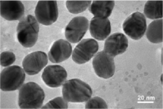
In this paper we analyze a mixture of gold NPs in a water solution. In order to analyze the morphological characteristics, NPs are sampled from this solution onto a very thin layer of carbon film. After the water evaporates, the two-dimensional morphology of NPs is measured using an Electron microscopy such as TEM. In our case, a JEOL high resolution TEM operating at kV accelerating voltage was used, which has nm of point resolution. The TEM shoots a beam of electrons onto the materials embedded with NPs and captures the electron wave interference by using a detector on the other side of the material specimen, resulting in an image. The electrons cannot penetrate through the NPs, resulting in a darker area in that part of the image. The output from this application will be an eight bit gray scale image where darker parts indicate the presence of a nanoparticle. The gray scale intensity is varying as an integer between and . Refer to Figure 1 for examples of TEM images.
 |
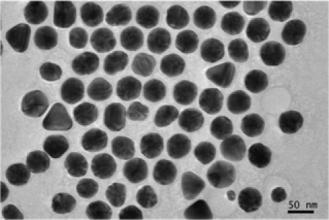 |
| (a) Gold nanoparticles at 20 nm | (b) Gold nano particles at 50 nm |
Due to the absorption of electrons by the gold atoms, the regions occupied by the NPs look darker in the image. The darkness pattern may vary according to specific arrangements of the atoms inside any single nanoparticle. Additionally, one can see many tiny dark dots in the background, which are uniformly distributed throughout the image region. These dark dots are generated because the carbon atoms of the carbon film also absorb electrons. One may also notice a white thin aura wrapping around the whole or partial boundary of a particle. This is the result of having surfactants on the rim of the particles. The surfactants are added to keep the particles from aggregating in the process of making colloidal gold. Analyzing the shapes of the NPs in a TEM image is primarily based on modeling them as objects, whose shapes are parametrized. Treating a nanoparticle as an object is the critical component of our modeling framework, which we discuss in the next section.
3 Object specification
An object is specified in a series of steps that allow us to model a wide variety of shapes. They are as follows: (a) template, (b) shift, scale and rotate operators, (c) object multiplicity. We discuss each of them in detail below.
3.1 Template
A template is a predetermined shape which is defined by a set of parameters which we call pure shape parameters or simply pure parameters. We will call the template a pure object and we will specify a pure object by its pure parameters as , where is the number of parameters, and it varies from shape to shape. For example, a circle with unit radius at the origin can be regarded as a template for circular objects. Likewise, an equilateral triangle with unit sides, centered at the origin with the median aligned to the x-axis, can be a template for triangular objects. We can potentially differentiate an equilateral triangle from an isosceles triangle even when they both belong to the triangle family. However, to avoid defining an infinite number of templates, we consider all types of a particular shape to be members of the same template. For example, all types of triangles, such as equilateral, right-angled, etc., are considered to be members of the triangle template. As such, when we refer to a template in this paper we refer to a family of shapes that has certain characteristics. A family of shapes is formed by deforming some of the pure parameters in the shape definition. We distinguish parameters as random (unknown) and constant (known) . The random pure parameters cannot be determined exactly by the template or by other components of . These random pure parameters affect the overall shape, size and other geometric properties, thereby causing a large scale deformation of the template. These parameters are closely related to the template, but for simplicity we ignore the indicator and use the notation . The pure parameters are chosen such that the defined template will have an area equal to the area of a unit circle, that is, square units. A template can be shifted, rotated and scaled, still belonging to the same shape family.
We also specify landmarks as the equally spaced boundary points of a given template. These landmarks can be determined if one knows the pure parameters. The landmarks will help us in representing the shape of the real image. In polar coordinates, these landmarks can be represented as
where is the distance of the th landmark from the center and is the rotation of the th landmark with respect to the baseline. The particular choice of the coordinate system in which the landmarks are represented does not affect the results. Hence, we have chosen to use polar coordinates for the simplicity of the mathematical analysis. In this paper we chose ninety landmark points for all the shapes. Simply speaking, these landmarks in an image form the shape. The random deformation of these landmarks results in small scale deformation of the template. In this paper, we focus our attention on the large scale deformation since the main goal is to determine the shape and not making boundary detection or contour tracking, where small-scale deformations are important. Templates used in the current study are given in (A) in the online supplementary material [Konomi et al. (2013)].
3.2 Shift, scale and rotation operators
Apart from the parameters that determine the shape which varies from template to template, there are also some common parameters related to shifting, rotating and scaling which are needed to represent the actual shape in the image. A particular affine shape with shift , scale and rotation is given by the landmarks , whose polar coordinates are
for .
3.3 Object multiplicity and the Markov point process
In an image we have multiple objects with different shapes and we assume that the number of objects is unknown. A point process is used to model the unknown number of objects and the overlapping. One of the widely used models that penalize object overlapping is based on the Markov Point Process (MPP) [Ripley and Kelly (1977)] representation of objects. In particular, the Area Interaction Process Prior (AIPP) [Baddeley and van Lieshout (1993), Mardia et al. (1997)] penalized the area of overlap between any two objects. Below, MPP representation details are given. The location parameters , the points in the MPP representation and the number of objects are modeled as
| (1) |
where denotes the area of the image covered by more than one object, is a collection of parameters that represents the th object and represents these parameters for all objects which we call “object parameters”, is the normalizing constant which depends on all the parameters described above and the positive unknown parameters and []. The interaction parameter controls the overlapping between objects and the number of objects in the image. For example, does not penalize overlapping, whereas does not allow overlapping at all. Prior distributions for and are considered in subsequent sections. Another way to penalize object overlapping is the two-way interaction:
The indicator term will not allow three or more objects to overlap in the same area, is the region of a single object characterized by its parameters and is the overlapping area between the th and the th object. We can generalize this case to allow more objects to overlap in a region and also penalize with a different parameter . Investigating such models is out of the scope of this paper. For notational convenience, we introduce to represent the MPP parameters and define , , , to be used subsequently.
4 Model
4.1 The likelihood function
Due to the electron absorption, the mean intensity of the background is larger than the mean intensity of the regions occupied by the NPs. Furthermore, since each nanoparticle has different volume size, the mean pixel intensity for each nanoparticle is different, which is evident from the representative TEM images of gold NPs shown in Figure 1. It can also be observed that the overlapping regions usually have lower intensity because they absorb more electrons in that region. For tractability, we consider the darkest region to be the dominant region in determining the configuration of the objects with which it is overlapping. Due to specific arrangements of the atoms inside any single nanoparticle, the neighboring pixels have similar intensities. An appropriate choice for the covariance function in such scenarios is the popular Conditional Autoregressive (CAR) model [Cressie (1993)]. Computationally, a much simpler model is the independent noise model [Baddeley and van Lieshout (1993), Mardia et al. (1997), Rue and Hurn (1999)].
After analyzing both real and simulated data sets, the posterior specification of the parameters did not change much even if we replaced the CAR model with the independent Gaussian noise model. An added advantage with the independent Gaussian noise model is that it is a lot simpler. We denote as the mean vector and as the variance vector for the background and objects intensity. To facilitate the notation, we use . In this case the likelihood can be written as
| (2) |
where is the number of pixels, is the th pixel, is the mean of the th pixel, is the function of the variance depending on the pixel and is the intensity of the th pixel. More explicitly, the mean intensity for pixels covered by more than one object is taken to be the minimum mean intensity of the objects covering the pixels and with variance which corresponds to the variance of that object.
For example, in the case where we allow only two-way interaction, equation (2) can be written as
| (3) | |||
where is the region occupied by all objects (NPs) without the th object and is the area of the background.
4.2 Prior specification
We elicit the joint prior distribution hierarchically as follows:
In the above expression is the prior of the means and the variances of the background and the objects, is the joint prior of the locations and the number of the objects as given in equation (), is the joint prior on all the “object parameters” except the locations and is the prior on the interaction parameters.
We assume independent pairs and assign a noninformative prior for each of these pairs:
| (5) |
All the “object parameters” except the locations are assumed to be independent from object to object. Also, the scale, rotation and template within the object parameters are assumed to be independent of other parameters while is assumed to be closely related to the template (shape). We remind the reader that are different from template to template. In mathematical form we have
| (6) |
We assign a uniform prior for which is proportional to the size of the image , that is, . All other shapes, except circles, have a rotation parameter . The prior density for is , which favors values near and . The circle and square do not have a random pure parameter, while the other considered templates have at least one random pure parameter. All these parameters have one basic characteristic: they are constrained to take values between two variables . We use altered location and scale Beta distribution as a prior given by
where are different for the three different cases. Furthermore, we have used the uniform discrete distribution to specify the prior for the template, .
For both the object process parameters we assume independent log-normal distribution priors with parameters which determine a mean close to and large variance, , . We calibrated priors such that inference is as invariant as possible to changes in the image resolution by defining parameters in physical units rather in terms of pixels, and tried to retain their physical interpretation wherever possible. For example, when we zoom out of an image, we may see a great number of objects in the purview, and the perceived.
4.3 The posterior distribution
The model proposed above is a hierarchical model of the form
| (7) | |||||
where are known values, is a random intractable normalizing constant and is the MPP prior without the normalizing constant.
The posterior distribution of the parameters is proportional to the product of (a), (b) and (c) in the above hierarchical representation:
| (8) | |||
We use the Markov chain Monte Carlo (MCMC) computation algorithm to carry out the inference since the posterior distribution is analytically intractable and the point process prior has a random intractable normalizing constant. To facilitate the discussion, we call the pseudo posterior distribution.
5 Posterior computation using MCMC
The MCMC algorithm used in this paper can be described as a two-stage Metropolis–Hastings algorithm. We first sample the parameters from the pseudo posterior distribution followed by a Monte Carlo Metropolis–Hastings step to account for [Liang and Jin (2011), Liang, Liu and Carroll (2010)].
The MCMC algorithm will have the following form:
-
•
Given the current state draw from using any standard MCMC sampler.
-
•
Given all the parameters, simulate auxiliary variables from the likelihood using an exact sampler.
-
•
Estimate as
which is also known as the importance sampling (IS) estimator of .
-
•
Compute (estimate) the MH rejection ratio as
(9) The last equation is true since . So, the above approximates the normalizing constant of the posterior.
-
•
Accept with probability .
Simulating auxiliary variables from the likelihood is straightforward and simply requires us to sample from normal distribution with parameters defined at the proposed state of the sampler. The challenge lies in drawing from the pseudo posterior.
A generalized Metropolis-within-Gibbs sampling with a reversible jump step is used to simulate from the pseudo posterior distribution with known number of objects. Additionally, a reversible jump MCMC (RJ-MCMC) with spatial birth-death as well as merge-split move is invoked to sample the number of objects and their corresponding parameters.
We draw from the joint pseudo posterior by alternately drawing from the conditional pseudo posteriors of , and as follows:
-
•
Draw from using a Metropolis-within-Gibbs sampler.
-
•
Draw from the pseudo posterior using a RJ-MCMC.
-
•
Draw from the distribution using an M–H step.
We explain these steps in detail, in the following paragraphs.
5.1 Updating , given and
The conditional distribution of does not have any closed form and the same is true for the conditional distribution of every component or group of components of . A Gibbs sampling step which contains Metropolis–Hastings steps and RJ-MCMC steps is utilized. In the online supplementary material (B) [Konomi et al. (2013)] we give the Metropolis–Hastings updates for excluding , which is given next.
5.1.1 Updating the template (swap move)
We can view the problem of shape selection as a problem of model selection between , where represents the model with template . Moving from shape to shape is considered a difficult task since not only the pure parameters that characterize the template are different, but also the parameter specification may not have the same meaning across templates. For example, one can argue that the scaling parameter of a circle can be different from the scaling parameter of a triangle. The move from shape to shape is based on the rule that both shapes should have the same area and the centers of both shapes are the same. This increases the likelihood of generating good proposals. For the particular shapes we deal with, the equality of area also means equality of the scaling parameter. This means that all of the above models have the same scaling and location parameters. The rotation parameter, , can be chosen such that the proposed shape overlap “matches” as much as possible to the existing shape given the same or simply one may retain the same while changing shapes. The pure random parameters are the only parameters that do not have a physical meaning when we change the shape and also their number could vary from shape to shape. Reversible Jump MCMC is used successfully for problems with different dimensionality and is characterized by introducing auxiliary variables for the unmatched parameters [Green (1995)]. This is the approach we follow in this paper. For more details see Appendix A.
5.2 Updating
Two different types of moves are considered in updating the number of objects: birth-death and split-merge. In the death step, one chosen-at-random object is deleted and in the birth step, one object with parameters generated from the priors is added. In the merge step we consider the case where two objects die and give birth to a new one and in the split step two new objects are created in the place of one. For more detail see Appendix B.
5.3 Updating
The random walk -normal proposal is used to sample from the pseudo posterior distribution of , .
6 Simulations
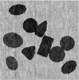
In this section we use a simulation study to evaluate the performance of our proposed MCMC method. We consider two examples wherein a image with ten objects each are generated from the prior distributions described in Section 4.2 with area interaction parameter and , respectively. The pixels inside each object have constant mean, which is different from object to object. The covariance matrix is chosen from a CAR model with parameters very close to the extreme dependence. Objects in both the example images have different morphological properties and belong to the five different shape families described in Section 2. The image used in the first example is shown in Figure 2(a) and the second is shown in Figure 2(b). For the
 |
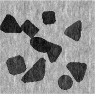 |
| (a) | (b) |
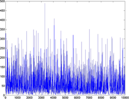
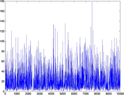
example images, the MCMC samples drawn from the posterior distribution of are given in Figure 3. From these simulations, we can see that the Markov chain mixes well and the posterior mean is close to the true values we used to simulate the data. Values close to are drawn in example 1 [Figure 1(a)], while values close to are drawn in example 2 [Figure 2(b)]. A general observation in the
 |
 |
| (a) posterior | (b) posterior |
simulations is that the variance of the posterior distribution of depends on the value of . For large values of we observe relatively larger posterior variance than for small values. Another significant observation is that there is a dependence on the accuracy and the variance of the posterior distribution of on the number and size of objects. To investigate this phenomenon, we fixed the value of but simulated images with a different number of objects and sizes. As we increase the number and the size of objects, the posterior distribution of will be closer to the true value. Below, we discuss two features of our method using the two examples.
6.1 Unknown AIPP parameters
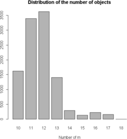
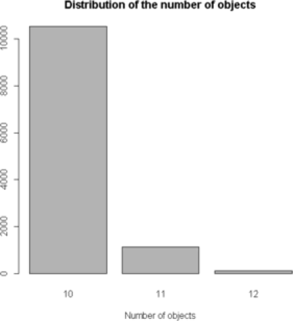
We demonstrate one of the advantages of treating the AIPP parameters as unknown. First, we compare the MCMC results from the proposed model with the results of the model that does not penalize overlapping. More specifically, we treat as a random variable in the first scenario, and then consider it known and misspecified in the second scenario. In both the runs, the parameter is set to its true value . The MCMC posterior distribution of for the image in Figure 2(a), in a total of iterations, is recorded and presented for these two different cases in Figure 4. The distribution of the number of objects in the case
 |
 |
| (a) | (b) random |
of is mostly a misspecification of the real image. In this case we have a sample of up to objects, which is almost twice the original number of objects. An obvious overestimation of the number of objects in the posterior distribution occurs when we do not penalize the overlapping. On the other hand, when we choose as a random variable of the posterior simulated number of objects represent the true number of objects. Treating as unknown, in comparison with , yields a better fit and improves classification. For the case where is fixed at a value different from zero, the answer depends on how close the original and the assumed value of are. If we fix the value of in the range determined from the MCMC updates, the results on the number of particles and shape analysis are not very different from the original values. Nevertheless, values outside the range can change the results dramatically. The same observations are true for the second simulated image [Figure 2(b)] as well.
6.2 Split and merge moves
Another feature of our proposed method is the split and merge type of move. We can see the merge and split step in action in Figures 5 and 6, respectively. In the absence of this type of move, it would have required a large number of MCMC iterations to arrive at the configurations shown. We present the two different move
 |
 |
| (a) th iteration | (b) th iteration |
steps that occurred in the two simulated images. The th and the th MCMC iteration is given for the first image. In addition to different changes that have occured, there is an obvious merge move step, wherein the seventh and eighth objects in Figure 5(a) are merged to form the seventh object in
 |
 |
| (a) th iteration | (b) th iteration |
Figure 5(b). Similarly, we show the split move in action using example 2. Snapshots taken at the th and the th MCMC iterations for example 2 are given in Figure 6(a) and (b). Not only an obvious split step has occurred but also we can see the different deviations of the boundaries which are related to the object representation parameters.
6.3 Implementation details
All the simulations and the algorithms were implemented in MATLAB, running on a Xeon dual core processor clocking GHz with GB RAM. MCMC chains are initialized by using classical image processing tools. All the five templates are randomly assigned to complete template specification. The simulation time for the two examples is approximately two hours for iterations. Convergence of the chains was observed within the first iterations. However, we point out that the computational time of the proposed method depends on the size of the image, the number of the objects and the complexity of overlapping, and burn-in time which strongly depends on the initial state of the chain.
In order to accelerate quick mixing, we take advantage of several classical image processing tools. Notable among these are the watershed image segmentation and certain morphological operator based image filtering techniques such as erosion, dilation etc. [Gonzalez and Woods (2007)]. For example, we use watershed segmentation to decompose the image into subimages that have approximately nonoverlapping regions (in terms of objects). A repeated application of the erosion operator on the subimages, in conjunction with connected-component analysis and dilation operation, gives us an approximate count of number of objects and their morphological aspects. Such information can be used to initialize the chains and to construct proposal distributions required by the MCMC sampler. In addition, the region-based approach allows one to exploit distributed and parallel computing concepts to reduce simulation time and make the algorithm scalable. Further details are not presented here since morphological preprocessing is not the subject of the present work. We point out above that choices affect simulation time and may improve mixing but otherwise are not necessary for our proposed method to work. In addition, simulation time and effort required by the MCMC method required are relatively small compared to the time, effort and resources required to produce the NPs and finally obtain the TEM images which can exceed weeks.
7 Application to gold nano particles
Using the MCMC samples, we can obtain the distribution of the particle size, which is characterized by the area of the nanoparticle and the distribution of the particle shape. The aspect ratio, defined as the length of the perimeter of a boundary divided by the area of the same boundary, can be derived from the combination of size, shape and the pure parameters. The statistics of size, shape and aspect ratio are widely adopted in nano science and engineering to characterize the morphology of NPs, and are believed to strongly affect the physical or chemical properties of the NPs [El-Sayed (2001), Nyiro-Kosa, Nagy and Posfai (2009)]. For example, the aspect ratio is considered as an important parameter relevant to certain macro-level material properties because physical and chemical reactions are believed to frequently occur on the surface of molecules so that as the aspect ratio of a nanoparticle gets larger, those reactions are more active.
We apply our method to three different TEM images. The parameters that maximize the posterior distribution (MAP) obtained from the (MCMC) are presented in detail. Our classification results of particular type are verified by our collaborators with domain expertise; this manual verification appears the only valid way for the time being. More than of the NPs in those images are classified correctly. This also includes the particles in the boundary as well as having overlapping regions. For completely observed objects, there is almost correct classification.
We start our application with the image in Figure 1(a). Morphological image processing operations, such as watershed transformation and erosion, can be used to get an approximate count of the number of NPs in the model [Gonzalez and Woods (2007)]. They also can be used in initializing the MCMC chains and in constructing proposal distributions required by the MCMC sampler. The morphological image processing we used in this dissertation has the following steps: (1) image filtering and segmentation, (2) determining the number of objects, (3) estimating location, size and rotation parameters. We first transform the image from grey to a binary image and then apply watershed transformation to partition the image into subimages. In each binary subimage we apply erosion and dilation operations to find initial values for the parameters inside of each subimage. Because this morphological processing is not the subject of the present work, it is not presented in more detail. After the initial values are obtained from the preprocessing step, all five templates are randomly assigned for starting template specifications. From the MCMC sampler described in Section 5 we obtain a random sample of the posterior distribution for all the parameters which characterize the NPs, namely, the shape , the size , the rotation , the random pure parameter , the mean intensity and the variance . We use this posterior sample for inferring the model parameters and extracting the morphological information of NPs with uncertainty in shape size and classification. To better present our results, we chose to work with the Maximum a posteriori (MAP) estimations of these parameters.
 |
 |
| (a) (scale) | (b) (foreground intensity) |
|
|
| (c) (random pure parameter) | |
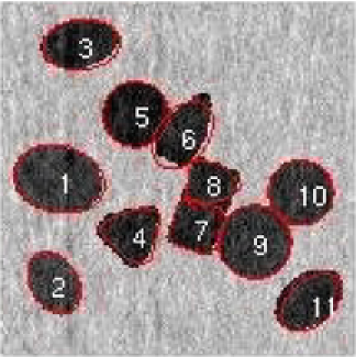
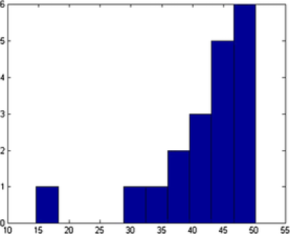
In Figure 7 we show the TEM image and MAP estimates of the parameters for MCMC sample. In Figure 8 we present the parameters of , and that correspond to the MAP estimate for all the number of objects, , corresponding to that value. Summary statistics of the shape parameters are given in Table 1. From the table and the histogram it is clear that the mean intensity is different from nanoparticle to nanoparticle, justifying our assumption of different means in (4.1). We also obtain the posterior probability of the classification for each of the objects. This probability depends on the complexity of the shape of the object. For example, object has been classified as an ellipse with probability , whereas object has been classified as an ellipse with probability (circle with probability ). In Table 1 (and in all the following tables of this chapter) we presented the classification with the highest posterior probability of some of the nanopartiles. In this example we successfully deal with the object overlapping and objects laying on the boundaries.
| Object | Shape | Center | Size | Rotation | Mean | |
|---|---|---|---|---|---|---|
| 1 | E | 51.49 | 1.14 | 50.64 | ||
| 2 | E | 49.41 | 1.22 | 74.67 | ||
| 3 | E | 47.20 | 1.12 | 62.55 | ||
| 4 | E | 28.86 | 1.15 | 71.58 | ||
| 5 | E | 49.98 | 1.13 | 64.58 | ||
| 6 | C | 51.82 | NA | NA | 73.76 |
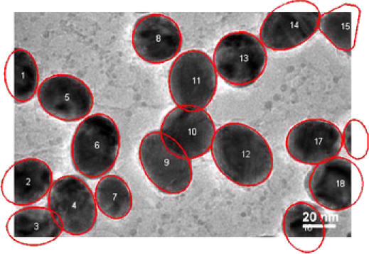
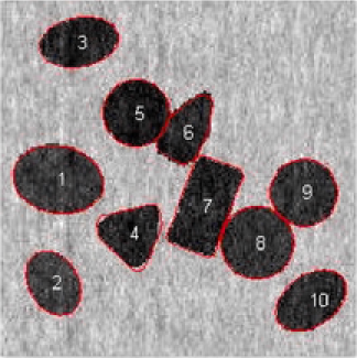
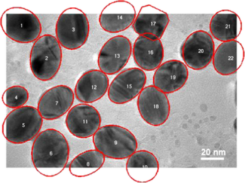
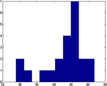
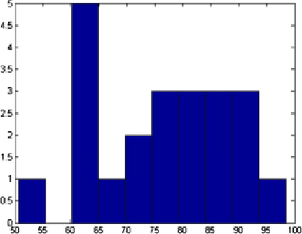
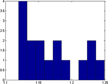
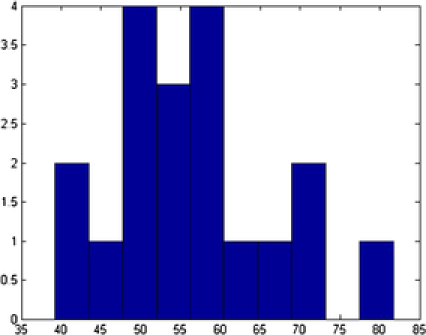
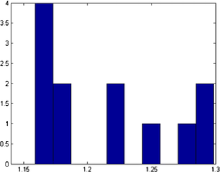
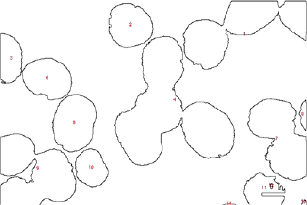
Our second application deals with a more complex image shown in Figure 9. In this image at least overlapping areas and at least nanoparticles laying in the boundary are observed. More specifically, nanoparticles , , , , , , , and lay in the boundary of the image while pairs 2–4, 3–4, 9–10, 10–11, 17–18, and 10–12 overlap. In this example, the overlapping is more complex and existing methods fail to represent the real situation. A number of nanoparticles are overlapped together forming a groups such as nanoparticles 9–10–11–12. MAP estimate values for all the parameters are obtained after MCMC iterations. Complex shapes have been classified accurately; see Figure 9. For example, nanoparticle has an incomplete image and it has been classified as a circle with posterior probability . The MAP estimates of the parameters drawn from MCMC, namely, shape , size , rotation , random pure parameter and mean intensity are presented for the first six objects in Table 2. In this application, out of the objects are ellipses (E) and are circles (C) and one is a triangle (TR). We also present the histogram of the MAP estimates of parameters , and in Figure 10. Summary statistics of various shape parameters are given in Table 2. We see from the table that our proposed algorithm captures triangles, circles etc. quite accurately.
| Object | Shape | Center | Size | Rotation | Mean | |
|---|---|---|---|---|---|---|
| 1 | E | 37.48 | 1.2960 | 39.185 | ||
| 2 | C | 41.04 | NA | NA | 42.969 | |
| 3 | E | 38.02 | 1.2175 | 52.569 | ||
| 4 | E | 47.44 | 1.1591 | 60.605 | ||
| 5 | E | 44.33 | 1.1612 | 51.080 | ||
| 6 | E | 49.63 | 1.1621 | 44.617 |
 |
 |
| (a) (scale) | (b) (foreground intensity) |
|
|
| (c) (random pure parameter) | |
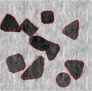
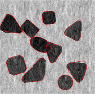
Our next application deals with an image with nanoparticles with shapes; see Figure 1(b). In this image, few objects have overlapping areas and at least nanoparticles are laying in the boundary. Some objects do not have very clear shape like objects and .
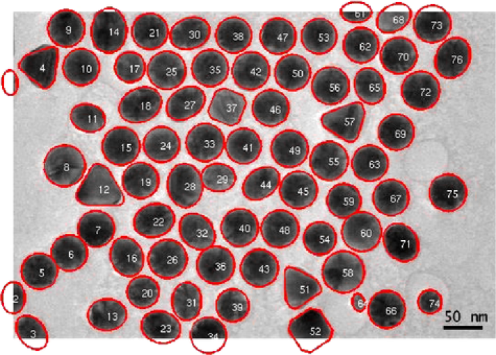
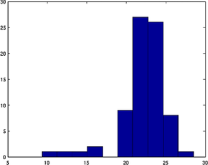
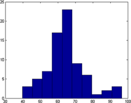
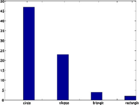
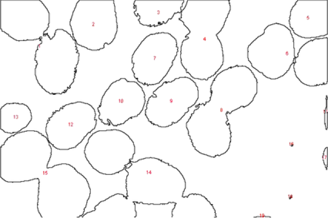
Different shapes are captured with different templates with the proposed method. In addition to the circles and ellipses which were successfully captured in the previous images, the triangles and squares are also captured accurately. Nanoparticles denoted by and are classified correctly, even if they have vague shapes; see Figure 11. In this example, out of nanoparticles, are classified as a circle, as an ellipse, as a triangle and as a square. Distribution of the various parameters of the identified objects are shown in Figure 12. In Table 3 we present all the triangular shapes in order to compare the pure parameter . As we can see from the table, triangular shape nanoparticles and are closer to the equilateral triangle, with value close to , while triangular shape nanoparticles and have wider sides, since their .
 |
 |
| (a) (scale) | (b) (foreground intensity) |
|
|
| (c) (shape classification) | |
| Object | Shape | Center | Size | Rotation | Mean | |
|---|---|---|---|---|---|---|
| 1 | E | 12.43 | 1.29 | 66.27 | ||
| 4 | 25.82 | 2.32 | 49.33 | |||
| 12 | 28.73 | 2.31 | 79.59 | |||
| 28 | E | 24.09 | 1.14 | 68.19 | ||
| 51 | 24.61 | 2.25 | 63.29 | |||
| 57 | 25.25 | 2.01 | 70.49 |
In this image we can see more than percent of the nanoparticles are in the same shapes like circular or slightly tilted like ovals. Normally when we do shape controlled synthesis, we called it nano spheres or circular nanoparticles. Approximately five to ten percent of the other shapes or slight changes we usually neglect because in solution synthesis routes it is very difficult to synthesis of the same size and same shapes. However, if we consider critically the reason of shape evolution or statistical analysis of different shapes, then this small difference might be considered. We classify this particular example as spherical gold nanoparticles having almost the same size and shapes.
As a part of the verification process, we compare the accuracy of our method with that of the current practice used in nanoscience. In brief, the current practice is largely a manual process with support of image processing tools such as ImageJ Particle Analyzer (http://rsbweb.nih.gov/ij) and AxioVision (http://www.zeiss.com/), which have been popularly used for biomedical image processing. The results are shown in Figures 13 and 14.
The manual counting process, subject to the application of the above imaging tools, is necessitated by the low accuracy of the autonomous procedures. For three TEM images with overlaps among particles, our procedure recognized of the total articles compared to the 20–50% recognition rate of the ImageJ. Considering frequent occurrence of overlaps in the TEM images of nanoparticles, the existing software cannot be used as more than a supporting tool. We have also applied our method to other images with the same success, encouraging its applicability.
8 Conclusion
We adopted a Bayesian approach to image classification and segmentation simultaneously and applied it in TEM images of gold nanoparticles. The merit of our development is to provide a tool for nanotechnology practitioners to recognize the majority of the nanoparticles in a TEM image so that the morphology analysis can be performed subsequently. This can evaluate how well the synthesis process of nanoparticles is controlled, and may even be used to explain or design certain material properties. Several factors like kinetic and thermodynamic parameters, flux of growing material, structure of the support, presence of defects and impurities can affect the morphology of NPs. In the future, we are planning to perform a factorial type experiment to identify the significant factors for morphological study. These significant factors can be properly controlled to develop NPs of required shapes.
From the experimental point of view, several improvements of existing techniques will be helpful to characterize the shape of the NPs. One is TEM tomography that allows to image an object in three dimensions, by automatically taking a series of pictures of the same particle at different tilt angles [Midgley and Weyland (2003)]. Another improvement of TEM is environmental HRTEM that is able to image nanoparticles, with atomic lattice resolution, at various temperatures and pressures [Hansen et al. (2002)].
From the modeling point of view, we used marked point process to represent the NPs in the image, where points represent the location of NPs and marks represent their geometrical features. More specifically, we treated the NPs in the image as objects, wherein the geometrical properties of the object were largely determined by templates and the interaction between the objects was modeled using the area interaction process prior. By varying the template parameters and applying operators such as scaling, shifting and rotation to the template, we modeled different shapes very realistically. In our current applications, we chose circle, triangle, square and ellipse as our templates. Other templates can be also constructed in the same framework. To solve the intractability of the posterior distribution, we proposed a complex Markov chain Monte Carlo (MCMC) algorithm which involves Reversible Jump, Metropolis–Hastings, Gibbs sampling and a Monte Carlo Metropolis–Hastings (MCMH) for the intractable normalizing constants in the prior. The first steps deal with simulating from a pseudo posterior distribution without involving the random normalizing constant. A generalized Metropolis-within-Gibbs sampling with a reversible jump step is used to simulate from a pseudo posterior distribution given the number of objects. Additionally, a reversible jump MCMC with the use of birth-death and merge-split moves is invoked on moving from a state with a different number of objects. Finally, we simulate from the intractable normalizing constant posterior using Monte Carlo Metropolis–Hastings where the acceptance ratio of the sample taken from the pseudo posterior is estimated by simulating from an auxiliary variable. We reported the posterior summary statistics of the shapes and the number of objects in the image. We successfully applied this algorithm to real TEM images, outperforming convention tools aided by manual screening. Our proposed methodology can help practitioners to associate morphological characteristics to physical and chemical properties of the NPs, and in synthesizing materials that have potential applications in optics and medical electronics, to name a few.
Appendix A Swap move
Two new variables are introduced to make it clear that the pure parameters have a different meaning from template to template. For all the shapes, we provide a general algorithm: Let denote the current state and the proposed state for . The notation of the parameters is different from the previous sections to show the dependence of the parameters on the model (or template). If , generate from the prior distribution of the and consider a bijection: . From this bijection it is clear that the Jacobian is equal to identity matrix, , and . In summary, the RJ-MCMC algorithm is as follows:
-
•
Select model with probability .
-
•
Generate from .
-
•
Set .
-
•
Compute the M–H ratio:
where is the Jacobian.
-
•
Set with probability and otherwise.
Appendix B Birth, death, split and merge moves
Let , , and be the probabilities of proposing a birth, death, split or a merge move, respectively.
B.1 Birth and death pair of moves
In the birth step a new object is proposed with a randomly assigned center. In this step we increase the dimension of the parameters by , all the parameters which describe the proposed object ). All these new parameters are sampled from the prior distributions of the parameters. The introduction of these kind of auxiliary variables leads again to a Jacobian equal to and the M–H ratio is
| (10) |
The death proposal chooses one object, , at random and removes it from the configuration. The M–H ratio for this move is similar to (9).
B.2 Split and merge pair of moves
The details for the split and merge move are more complicated than the move types described above. First we restrict our attention only to the case where we merge two neighboring objects or split one object into two neighbors. The distance between the two neighbors can be approximated by a function of their individual size. When we move from one state to another, we require that the proposed objects have equal area with the existing. In order for the Markov chain to be reversible we should ensure that every jump step can be reversed. We can improve the acceptance rate of these moves with different proposed algorithms, for example, Al-Awadhi, Jenninson and Hurn (2004), but that is beyond the scope of this paper.
To facilitate the representation, we will denote by bold characters , and the current state in every move and , and the current state values without the objects.
Merge step: Lets suppose we have two objects and that their parameters are . In the merge step, we move to a new object with parameters . The equation which links the sizes of the old objects with the new is . Also, and are chosen to represent the “weighted middle” point, taking in account the size of each object as . All the other parameters are chosen from one of the “parent” objects or at random.
In order to match the two dimensions, we introduce six auxiliary variables, , which not only would enable us to move from state to state but also are interpretable: is expressing the distance between two centers of the neighboring objects, is the angle created from the union of the two centers , is chosen such that and , , , .
The acceptance ratio, , in this case is the minimum of one and
| (11) |
where is the determinant of the Jacobian for the transformation and is the split proposed probability and is the merge proposed probability.
Split step: In the split step, we move from (, , , , , , , , , , , ) to , , , , , , , , , , , . In order to make this move possible, we introduce six proposal distributions for the auxiliary variables. We propose from the prior of the size parameter, from the prior of rotation parameter, from , from the priors of and , respectively. In order for this move to be reversible, we again use the same transform that was used in the merge step. With the same setting we can compute the M–H acceptance ratio.
Acknowledgments
We thank Professor Faming Liang for providing the preprint of his work on simulating from posterior distributions with doubly intractable normalization constants. We thank all the reviewers for their useful comments and a special thanks to the reviewer who helped us to improve the algorithm presented in page .
Templates and Metropolis–Hastings updates of
\slink[doi]10.1214/12-AOAS616SUPP \sdatatype.pdf
\sfilenameaoas616_supp.pdf
\sdescriptionDetails in MCMC algorithm.
References
- Al-Awadhi, Jenninson and Hurn (2004) {barticle}[mr] \bauthor\bsnmAl-Awadhi, \bfnmFahimah\binitsF., \bauthor\bsnmJenninson, \bfnmChristopher\binitsC. and \bauthor\bsnmHurn, \bfnmMerrilee\binitsM. (\byear2004). \btitleStatistical image analysis for a confocal microscopy two-dimensional section of cartilage growth. \bjournalJ. R. Stat. Soc. Ser. C. Appl. Stat. \bvolume53 \bpages31–49. \biddoi=10.1046/j.0035-9254.2003.05177.x, issn=0035-9254, mr=2037882 \bptokimsref \endbibitem
- Baddeley and van Lieshout (1993) {barticle}[author] \bauthor\bsnmBaddeley, \bfnmA. J.\binitsA. J. and \bauthor\bparticlevan \bsnmLieshout, \bfnmM. N. M.\binitsM. N. M. (\byear1993). \btitleStochastic geometry models in high-level vision. \bjournalJ. Appl. Stat. \bvolume20 \bpages231–256. \bptokimsref \endbibitem
- Blake and Yuille (1992) {bbook}[author] \bauthor\bsnmBlake, \bfnmA.\binitsA. and \bauthor\bsnmYuille, \bfnmA.\binitsA. (\byear1992). \btitleActive Vision. \bpublisherMIT Press, \blocationCambridge, MA. \bptokimsref \endbibitem
- Chen and Shao (1998) {barticle}[mr] \bauthor\bsnmChen, \bfnmMing-Hui\binitsM.-H. and \bauthor\bsnmShao, \bfnmQi-Man\binitsQ.-M. (\byear1998). \btitleMonte Carlo methods for Bayesian analysis of constrained parameter problems. \bjournalBiometrika \bvolume85 \bpages73–87. \biddoi=10.1093/biomet/85.1.73, issn=0006-3444, mr=1627238 \bptokimsref \endbibitem
- Chitrani, Ghazani and Chan (2006) {barticle}[author] \bauthor\bsnmChitrani, \bfnmDevika\binitsD., \bauthor\bsnmGhazani, \bfnmArezou\binitsA. and \bauthor\bsnmChan, \bfnmWarren\binitsW. (\byear2006). \btitleDetermining the size and shape dependence of gold nanoparticle uptake into mammalian cells. \bjournalNano Letters \bvolume6 \bpages662–668. \bptokimsref \endbibitem
- Cressie (1993) {bbook}[mr] \bauthor\bsnmCressie, \bfnmNoel A. C.\binitsN. A. C. (\byear1993). \btitleStatistics for Spatial Data, \bedition2nd ed. \bpublisherWiley, \blocationNew York. \bptokimsref \endbibitem
- El-Sayed (2001) {barticle}[pbm] \bauthor\bsnmEl-Sayed, \bfnmM. A.\binitsM. A. (\byear2001). \btitleSome interesting properties of metals confined in time and nanometer space of different shapes. \bjournalAcc. Chem. Res. \bvolume34 \bpages257–264. \bidissn=0001-4842, pii=ar960016n, pmid=11308299 \bptokimsref \endbibitem
- Gaponik et al. (2000) {barticle}[author] \bauthor\bsnmGaponik, \bfnmN. P.\binitsN. P., \bauthor\bsnmTalapin, \bfnmD. V.\binitsD. V., \bauthor\bsnmRogach, \bfnmA. L.\binitsA. L. and \bauthor\bsnmEychmüller, \bfnmA.\binitsA. (\byear2000). \btitleElectrochemical synthesis of CdTe nanocrystal/polypyrrole composites for optoelectronic applications. \bjournalJournal of Materials Chemistry \bvolume10 \bpages2163–2166. \bptokimsref \endbibitem
- Geyer and Møller (1994) {barticle}[mr] \bauthor\bsnmGeyer, \bfnmCharles J.\binitsC. J. and \bauthor\bsnmMøller, \bfnmJesper\binitsJ. (\byear1994). \btitleSimulation procedures and likelihood inference for spatial point processes. \bjournalScand. J. Stat. \bvolume21 \bpages359–373. \bidissn=0303-6898, mr=1310082 \bptokimsref \endbibitem
- Gonzalez and Woods (2007) {bbook}[author] \bauthor\bsnmGonzalez, \bfnmR. C.\binitsR. C. and \bauthor\bsnmWoods, \bfnmR. E.\binitsR. E. (\byear2007). \btitleDigital Image Processing, \bedition3rd ed. \bpublisherPrentice Hall, \blocationUpper Saddle River, NJ. \bptokimsref \endbibitem
- Green (1995) {barticle}[mr] \bauthor\bsnmGreen, \bfnmPeter J.\binitsP. J. (\byear1995). \btitleReversible jump Markov chain Monte Carlo computation and Bayesian model determination. \bjournalBiometrika \bvolume82 \bpages711–732. \biddoi=10.1093/biomet/82.4.711, issn=0006-3444, mr=1380810 \bptokimsref \endbibitem
- Hansen et al. (2002) {barticle}[author] \bauthor\bsnmHansen, \bfnmT. W.\binitsT. W., \bauthor\bsnmWagner, \bfnmJ. B.\binitsJ. B., \bauthor\bsnmHelveg, \bfnmS.\binitsS., \bauthor\bsnmRostrup-Nielson, \bfnmJ.\binitsJ., \bauthor\bsnmClausen, \bfnmB.\binitsB. and \bauthor\bsnmTopsoe, \bfnmH.\binitsH. (\byear2002). \btitleAtom resolved imaging of dynamic shape changes in supported copper nanocrystals. \bjournalScience \bvolume5546 \bpages1508–1518. \bptokimsref \endbibitem
- Hirsch et al. (2003) {barticle}[author] \bauthor\bsnmHirsch, \bfnmL. R.\binitsL. R., \bauthor\bsnmStafford, \bfnmR. J.\binitsR. J., \bauthor\bsnmBankson, \bfnmJ. A.\binitsJ. A., \bauthor\bsnmSershen, \bfnmS. R.\binitsS. R., \bauthor\bsnmRivera, \bfnmB.\binitsB., \bauthor\bsnmPrice, \bfnmR. E.\binitsR. E., \bauthor\bsnmHazle, \bfnmJ. D.\binitsJ. D., \bauthor\bsnmHalas, \bfnmN. J.\binitsN. J. and \bauthor\bsnmWest, \bfnmJ. L.\binitsJ. L. (\byear2003). \btitleNanoshell mediated nearinfrared thermal therapy of tumors under magnetic resonance guidance. \bjournalProc. Natl. Acad. Sci. USA \bvolume100 \bpages13549–13554. \bptokimsref \endbibitem
- ImageJ (2004) {bmisc}[author] \borganizationImageJ (\byear2004). \bhowpublishedImage processing and analysis in Java. Available at http://rsbweb.nih.gov/ij/. \bptokimsref \endbibitem
- Jana and Pal (1999) {barticle}[author] \bauthor\bsnmJana, \bfnmN. R.\binitsN. R. and \bauthor\bsnmPal, \bfnmT.\binitsT. (\byear1999). \btitleRedox catalytic property of still-growing and final palladium particles? A comparative study. \bjournalLangmuir \bvolume15 \bpages3458–3463. \bptokimsref \endbibitem
- Jana, Sau and Pal (1999) {barticle}[author] \bauthor\bsnmJana, \bfnmN. R.\binitsN. R., \bauthor\bsnmSau, \bfnmV.\binitsV. and \bauthor\bsnmPal, \bfnmT.\binitsT. (\byear1999). \btitleRedox catalytic property of still-growing and final palladium particles? A comparative study. \bjournalJ. Phys. Chem. B \bvolume103 \bpages115–121. \bptokimsref \endbibitem
- Jung, Ko and Nam (2008) {barticle}[author] \bauthor\bsnmJung, \bfnmM. R.\binitsM. R., \bauthor\bsnmKo, \bfnmJ. H. Shim B.\binitsJ. H. S. B. and \bauthor\bsnmNam, \bfnmJ. Y.\binitsJ. Y. (\byear2008). \btitleAutomatic cell segmentation and classification using morphological features and Bayesian networks. \bjournalProceedings of the Society of Photo-Optical Instrumentation Engineers \bvolume6813 \bpages202–212. \bptokimsref \endbibitem
- Kamat (1993) {barticle}[author] \bauthor\bsnmKamat, \bfnmP. V.\binitsP. V. (\byear1993). \btitlePhotochemistry on nonreactive and reactive (semiconductor) surfaces. \bjournalChemical Reviews \bvolume93 \bpages267–300. \bptokimsref \endbibitem
- Konomi et al. (2013) {bmisc}[author] \bauthor\bsnmKonomi, \bfnmBledar\binitsB., \bauthor\bsnmDhavala, \bfnmSoma S.\binitsS. S., \bauthor\bsnmHuang, \bfnmJianhua Z.\binitsJ. Z., \bauthor\bsnmKundu, \bfnmSubrata\binitsS., \bauthor\bsnmHuitink, \bfnmDavid\binitsD., \bauthor\bsnmLiang, \bfnmHong\binitsH., \bauthor\bsnmDing, \bfnmYu\binitsY. and \bauthor\bsnmMallick, \bfnmBani K.\binitsB. K. (\byear2013). \bhowpublishedSupplement to “Bayesian object classification of gold nanoparticles.” DOI:\doiurl10.1214/12-AOAS616SUPP. \bptokimsref \endbibitem
- Kothari, Chaudhry and Wang (2009) {barticle}[author] \bauthor\bsnmKothari, \bfnmS.\binitsS., \bauthor\bsnmChaudhry, \bfnmQ.\binitsQ. and \bauthor\bsnmWang, \bfnmM.\binitsM. (\byear2009). \btitleAutomated cell counting and cluster segmentation using concavity detection and ellipse fitting techniques. \bjournalIEEE International Symposium on Biomedical Imaging \bvolume1 \bpages795–798. \bptokimsref \endbibitem
- Kundu, Lau and Liang (2009) {barticle}[author] \bauthor\bsnmKundu, \bfnmS.\binitsS., \bauthor\bsnmLau, \bfnmS.\binitsS. and \bauthor\bsnmLiang, \bfnmH.\binitsH. (\byear2009). \btitleShape-controlled catalysis by cetyltrimethylammonium bromide terminated gold nanospheres. \bjournalJ. Phys. Chem. \bvolume113 \bpages5150–5156. \bptokimsref \endbibitem
- Kundu et al. (2003) {barticle}[author] \bauthor\bsnmKundu, \bfnmS.\binitsS., \bauthor\bsnmGhosh, \bfnmS. K.\binitsS. K., \bauthor\bsnmMandal, \bfnmM.\binitsM. and \bauthor\bsnmPal, \bfnmT.\binitsT. (\byear2003). \btitleReduction of methylene blue (MB) by ammonia in micelles catalyzed by metal nanoparticles. \bjournalNew Journal of Chemistry \bvolume27 \bpages656–662. \bptokimsref \endbibitem
- Liang (2010) {barticle}[mr] \bauthor\bsnmLiang, \bfnmFaming\binitsF. (\byear2010). \btitleA double Metropolis–Hastings sampler for spatial models with intractable normalizing constants. \bjournalJ. Stat. Comput. Simul. \bvolume80 \bpages1007–1022. \biddoi=10.1080/00949650902882162, issn=0094-9655, mr=2742519 \bptokimsref \endbibitem
- Liang and Jin (2011) {bmisc}[author] \bauthor\bsnmLiang, \bfnmF.\binitsF. and \bauthor\bsnmJin, \bfnmI. H.\binitsI. H. (\byear2011). \bhowpublishedA Monte Carlo Metropolis–Hastings algorithm for sampling from distributions with intractable normalizing constants. Technical report, Dept. Statistics, Texas A&M Univ., College Station, TX. \bptokimsref \endbibitem
- Liang, Liu and Carroll (2010) {bbook}[author] \bauthor\bsnmLiang, \bfnmF.\binitsF., \bauthor\bsnmLiu, \bfnmC.\binitsC. and \bauthor\bsnmCarroll, \bfnmR.\binitsR. (\byear2010). \btitleAdvanced Markov chain Monte Carlo Methods: Learning from Past Samples. \bpublisherWiley, \blocationChichester. \bidmr=2828488 \bptokimsref \endbibitem
- Link and El-Sayed (1999) {barticle}[author] \bauthor\bsnmLink, \bfnmS.\binitsS. and \bauthor\bsnmEl-Sayed, \bfnmM. A.\binitsM. A. (\byear1999). \btitleSize and temperature dependence of the plasmon absorption of colloidal gold nanoparticles. \bjournalJ. Phys. Chem. B \bvolume103 \bpages4212–4217. \bptokimsref \endbibitem
- Mardia et al. (1997) {barticle}[author] \bauthor\bsnmMardia, \bfnmK. V.\binitsK. V., \bauthor\bsnmQian, \bfnmW.\binitsW., \bauthor\bsnmShah, \bfnmD.\binitsD. and \bauthor\bparticlede \bsnmSouza, \bfnmK. M. A.\binitsK. M. A. (\byear1997). \btitleDeformable template recognition of multiple occluded objects. \bjournalIEEE Transactions on Pattern Analysis and Machine Intelligence \bvolume19 \bpages1035–1042. \bptokimsref \endbibitem
- Midgley and Weyland (2003) {barticle}[author] \bauthor\bsnmMidgley, \bfnmP. A.\binitsP. A. and \bauthor\bsnmWeyland, \bfnmM.\binitsM. (\byear2003). \btitle3D electron microscopy in the physical sciences: The development of Z-contrast and EFTEM tomography. \bjournalUltramicroscopy \bvolume96 \bpages13–431. \bptokimsref \endbibitem
- Møller et al. (2006) {barticle}[mr] \bauthor\bsnmMøller, \bfnmJ.\binitsJ., \bauthor\bsnmPettitt, \bfnmA. N.\binitsA. N., \bauthor\bsnmReeves, \bfnmR.\binitsR. and \bauthor\bsnmBerthelsen, \bfnmK. K.\binitsK. K. (\byear2006). \btitleAn efficient Markov chain Monte Carlo method for distributions with intractable normalising constants. \bjournalBiometrika \bvolume93 \bpages451–458. \biddoi=10.1093/biomet/93.2.451, issn=0006-3444, mr=2278096 \bptokimsref \endbibitem
- Murray, Ghahramani and MacKay (2006) {bmisc}[author] \bauthor\bsnmMurray, \bfnmI.\binitsI., \bauthor\bsnmGhahramani, \bfnmZ.\binitsZ. and \bauthor\bsnmMacKay, \bfnmD. J. C.\binitsD. J. C. (\byear2006). \bhowpublishedMCMC for doubly-intractable distributions. In Proc. 22nd Annual Conference on Uncertainty in Artificial Intelligence (UAI). Cambridge, MA. \bptokimsref \endbibitem
- Nyiro-Kosa, Nagy and Posfai (2009) {barticle}[author] \bauthor\bsnmNyiro-Kosa, \bfnmI.\binitsI., \bauthor\bsnmNagy, \bfnmD. C.\binitsD. C. and \bauthor\bsnmPosfai, \bfnmM.\binitsM. (\byear2009). \btitleSize and shape control of precipitated magnetite nanoparticle. \bjournalEuropean Journal of Mineralogy \bvolume21 \bpages293–302. \bptokimsref \endbibitem
- Pievatolo and Green (1998) {barticle}[mr] \bauthor\bsnmPievatolo, \bfnmA.\binitsA. and \bauthor\bsnmGreen, \bfnmPeter J.\binitsP. J. (\byear1998). \btitleBoundary detection through dynamic polygons. \bjournalJ. R. Stat. Soc. Ser. B Stat. Methodol. \bvolume60 \bpages609–626. \biddoi=10.1111/1467-9868.00143, issn=1369-7412, mr=1626009 \bptokimsref \endbibitem
- Qiang and Mardia (1995) {bmisc}[author] \bauthor\bsnmQiang, \bfnmW.\binitsW. and \bauthor\bsnmMardia, \bfnmK. V.\binitsK. V. (\byear1995). \bhowpublishedRecognition of multiple objects with occlusions. Research report, Dept. Statistics, Leeds. \bptokimsref \endbibitem
- Ripley (1977) {barticle}[mr] \bauthor\bsnmRipley, \bfnmB. D.\binitsB. D. (\byear1977). \btitleModelling spatial patterns. \bjournalJ. R. Stat. Soc. Ser. B Stat. Methodol. \bvolume39 \bpages172–212. \bnoteWith discussion. \bidissn=0035-9246, mr=0488279 \bptnotecheck related\bptokimsref \endbibitem
- Ripley and Kelly (1977) {barticle}[mr] \bauthor\bsnmRipley, \bfnmB. D.\binitsB. D. and \bauthor\bsnmKelly, \bfnmF. P.\binitsF. P. (\byear1977). \btitleMarkov point processes. \bjournalJ. Lond. Math. Soc. (2) \bvolume15 \bpages188–192. \bidissn=0024-6107, mr=0436387 \bptokimsref \endbibitem
- Rue and Hurn (1999) {barticle}[mr] \bauthor\bsnmRue, \bfnmHåvard\binitsH. and \bauthor\bsnmHurn, \bfnmMerrilee A.\binitsM. A. (\byear1999). \btitleBayesian object identification. \bjournalBiometrika \bvolume86 \bpages649–660. \biddoi=10.1093/biomet/86.3.649, issn=0006-3444, mr=1723784 \bptokimsref \endbibitem
- Sau, Pal and Pal (2000) {barticle}[author] \bauthor\bsnmSau, \bfnmT. K.\binitsT. K., \bauthor\bsnmPal, \bfnmA.\binitsA. and \bauthor\bsnmPal, \bfnmT.\binitsT. (\byear2000). \btitleSize regime dependent catalysis by gold nanoparticles for the reduction of eosin. \bjournalJ. Phys. Chem. \bvolume105 \bpages9266–9272. \bptokimsref \endbibitem
- Yu et al. (1997) {barticle}[author] \bauthor\bsnmYu, \bfnmYu-Ying\binitsY.-Y., \bauthor\bsnmChang, \bfnmSer-Sing\binitsS.-S., \bauthor\bsnmLee, \bfnmChien-Liang\binitsC.-L. and \bauthor\bsnmWang, \bfnmChris\binitsC. (\byear1997). \btitleGold nanorods: Electrochemical synthesis and optical properties. \bjournalJ. Phys. Chem. \bvolume301 \bpages6661–6664. \bptokimsref \endbibitem