Bayesian Optimization of Hyperparameters from Noisy Marginal Likelihood Estimates

Consider the standard BVAR model

where $\left\{\boldsymbol{\varepsilon}_{t}\right\}_{t=1}^{T}$ are iid $N(\boldsymbol{0},\boldsymbol{\Sigma})$. A simplified version of the Minnesota prior (see e.g. Karlsson, (2013)) without cross-equation shrinkage is of the form

with

where $\text{vec}(\underline{\boldsymbol{\Pi}})$ and $\underline{\boldsymbol{\Omega}}_{\Pi}$ denotes the prior mean and covariance of the coefficient matrix, $\underline{\boldsymbol{S}}$ is the prior scale matrix with the prior degrees of freedom, $\underline{\nu}$. The diagonal elements of $\underline{\boldsymbol{\Omega}}_{\Pi}$ are given by

where $\lambda_{1}$ controls the overall shrinkage and $\lambda_{3}$ the lag-decay shrinkage set by the user, $s_{r}$ denotes the estimated standard deviation of variable $r$. The fact that we do not use the additional cross-equation shrinkage hyperparameter, $\lambda_{2}$, makes this prior conjugate to the VAR likelihood, a fact that will be important in the following. It has been common practice to use standard values that dates back to Doan et al., (1984), but there has been a renewed interest to find values that are optimal for the given application (see e.g. Bańbura et al., (2010), Carriero et al., (2012) and Giannone et al., (2015)). Two main approaches have been proposed. First, Giannone et al., (2015) proposed to sample from the joint posterior distribution using the decomposition

where $\boldsymbol{\beta}=(\Pi,\Sigma)$ and $p(\boldsymbol{\theta}|\mathbf{y}_{1:T})$ is the marginal posterior distribution of the hyperparameters. The algorithm samples from $p(\boldsymbol{\theta}|\mathbf{y}_{1:T})$ using Metropolis-Hastings (MH) and then samples directly from $p(\boldsymbol{\beta}|\boldsymbol{\theta},\mathbf{y}_{1:T})$ for each $\boldsymbol{\theta}$ draw by drawing $\Pi$ and $\Sigma$ from the Normal-Inverse Wishart distribution. There are some limitations to using this approach. First, the $p(\boldsymbol{\theta}|\mathbf{y}_{1:T})$ can be multimodal (see e.g. the application in Section 6) and it can be hard to find a good MH proposal density, making the sampling time-consuming. Second, practitioners tend to view hyperparameter selection as similar to model selection and want to determine a fixed value for $\boldsymbol{\theta}$ once and for all early in the model building process.

Carriero et al., (2012) propose an exhaustive grid search to find the $\boldsymbol{\theta}$ that maximizes $p(\boldsymbol{\theta}|\mathbf{y}_{1:T})$ and then uses that optimal $\boldsymbol{\theta}$ throughout the remaining analysis. The obvious drawback here is that a grid search is very costly, especially if we have non-conjugate priors and more than a couple of hyperparameters.

A problem with both the approach in Giannone et al., (2015) and Carriero et al., (2012) is that for most interesting models $p(\boldsymbol{\theta}|\mathbf{y}_{1:T})$ is not available in closed form. Even the Minnesota prior with cross-equation shrinkage is no longer a conjugate prior and $p(\boldsymbol{\theta}|\mathbf{y}_{1:T})$ is intractable. In fact, most Bayesian models used in practice have intractable $p(\boldsymbol{\theta}|\mathbf{y}_{1:T})$, including the steady-state BVAR (Villani,, 2009) and the TVP-SV BVAR (Primiceri,, 2005) used in Section 5 and 6.

When $p(\boldsymbol{\theta}|\mathbf{y}_{1:T})$ is intractable, MCMC or other simulation based methods like Sequential Monte Carlo (SMC) are typically used to obtain a noisy estimate of $p(\boldsymbol{\theta}|\mathbf{y}_{1:T})$. Since

where $p(\mathbf{y}_{1:T}|\boldsymbol{\theta})=\int p(\mathbf{y}_{1:T}|\boldsymbol{\theta},\beta)p(\beta|\boldsymbol{\theta})d\beta$ is the marginal likelihood, this problem goes under the heading of (log) marginal likelihood estimation. We will therefore frame our method as maximizing the log marginal likelihood; maximization of $p(\boldsymbol{\theta}|\mathbf{y}_{1:T})$ is achieved by simply adding the log prior, $\log p(\boldsymbol{\theta})$, to the objective function.

Chib, (1995) proposes an accurate way of computing a simulation-consistent estimate of the marginal likelihood when the posterior can be obtained via Gibbs sampling, which is the case for many econometric models. We refer to Chib, (1995) for details about the marginal likelihood estimator and its approximate standard error.

Estimating the marginal likelihood for the TVP-SV BVAR is more challenging and we will adopt the method suggested by Chan and Eisenstat, (2018). The approach consists of four steps; 1) obtain a posterior sample via Gibbs sampling, 2) integrate out the time-varying VAR coefficients analytically, 3) integrate out the stochastic volatility using importance sampling to obtain the integrated likelihood, 4) integrate out the static parameters using another importance sampler. Since the algorithm makes use of two nested importance samplers, it is a special case of importance sampling squared ($IS^{2}$) (Tran et al.,, 2013); see Section 6 for more details.

There are many alternative estimators that can be used in our approach, for example, the extension of Chib’s estimator to Metropolis-Hastings sampling (Chib and Jeliazkov,, 2001), and estimators based on importance sampling (Geweke,, 1999) or Sequential Monte Carlo (Doucet et al.,, 2001).

All simulation-based estimators: i) give noisy evaluations of the marginal likelihood, ii) are time-consuming, and iii) have a precision that is controlled by the user in terms of the number of MCMC or importance sampling draws. The next section explains how traditional Bayesian optimization is well suited for points i) and ii), but lacks a mechanism for exploiting point iii). Taking the user controlled precision into account brings a new perspective to the problem and we propose a class of algorithms that handle all three points above.

Since Bayesian optimization is a relatively unknown method in econometrics, we give an introduction here to Gaussian processes and their use in Bayesian optimization.

A Gaussian process (GP) is a (possibly infinite) collection of random variables such that any subset is jointly distributed according to a multivariate normal distribution, see e.g. Williams and Rasmussen, (2006). This process, denoted by $f(\mathbf{x})\sim\mathcal{GP}(\mu(\mathbf{x}),k(\mathbf{x},\mathbf{x}^{\prime}))$, can be seen as a probability distribution over functions $f:\mathcal{X}\to\mathbb{R}$ that is completely specified by its mean function, $\mu(\mathbf{x})\equiv\mathbb{E}f(\mathbf{x})$, and its covariance function, $\mathbb{C}(f(\mathbf{x}),f(\mathbf{x}^{\prime}))\equiv k(\mathbf{x},\mathbf{x}^{\prime})$, where $\mathbf{x}$ and $\mathbf{x}^{\prime}$ are two arbitrary input values to $f(\cdot)$. Note that the covariance function specifies the covariance between any two function values, $f(\mathbf{x}_{1})$ and $f(\mathbf{x}_{2})$. A popular covariance function is the squared exponential (SE):

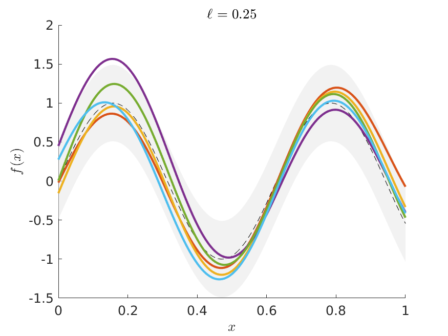
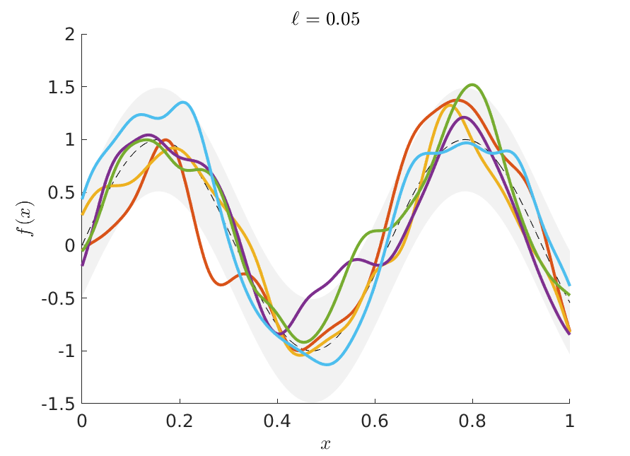
where $|\mathbf{x}-\mathbf{x}^{\prime}|$ is the Euclidean distance between the two inputs; the covariance function is specified by its two kernel hyperparameters, the scale parameter $\sigma_{f}>0$ and the length scale $\ell>0$. The scale parameter $\sigma_{f}$ governs the variability of the function and the length scale determines how fast the correlation between two function values taper off with the distance $|\mathbf{x}-\mathbf{x}^{\prime}|$, see Figure 1. The fact that any finite sampling of function values $\{f(\mathbf{x}_{n})\text{ for }\mathbf{x}_{n}\in\mathcal{X}\}_{n=1}^{N}$ constitutes a multivariate normal distribution on $\mathbb{R}^{N}$ allows for the convenient conditioning and marginalization properties of the multivariate normal distribution. In particular, this makes it easy to compute the posterior distribution for the function $f$ at any input $\mathbf{x}_{\star}$.

An increasingly popular alternative to the squared exponential kernel is the Matérn kernel, see e.g. Matérn, (1960) and Williams and Rasmussen, (2006). The Matérn kernel has an additional hyperparameter, $\nu$>0, in addition to the length scale $\ell$ and scale $\sigma_{f}$, such that the process is $k$ times mean square differentiable if and only if $\nu>k$. Hence, $\nu$ controls the smoothness of the process and it can be shown that the Matérn kernel approaches the SE kernel as $\nu\rightarrow\infty$ (Williams and Rasmussen, (2006)). Our approach is directly applicable for any valid kernel function, but we will use the popular Matérn $\nu=5/2$ kernel in our applications:

where $r=|\mathbf{x}-\mathbf{x}^{\prime}|$. The Matérn 5/2 has two continuous derivatives which is often a requirement for Newton-type optimizers (Snoek et al.,, 2012). The hyperparameters, $\sigma_{f}$ and $\ell$, are found by maximizing the marginal likelihood, see e.g. Williams and Rasmussen, (2006).

Consider the nonlinear/nonparametric regression model with additive Gaussian errors

and the prior $f(\mathbf{x})\sim\mathcal{GP}(0,k(\mathbf{x},\mathbf{x}^{\prime}))$. Given a dataset with $n$ observations, the posterior distribution of $f(\boldsymbol{x}_{\star})$ at a new input $\boldsymbol{x}_{\star}$ is (Williams and Rasmussen,, 2006)

where $\boldsymbol{y}=(y_{1},\ldots,y_{n})^{\top}$, $k(\boldsymbol{x}_{\star})$ is the $n$-vector with covariances between $f$ at the test point $\boldsymbol{x}_{\star}$ and all other training inputs, $\boldsymbol{K}(\boldsymbol{X},\boldsymbol{X})$ is the $n\times n$ matrix with covariances among the function values at all $n$ training inputs in $\boldsymbol{X}$. When the errors are heteroscedastic with variance $\sigma_{i}^{2}$ for the $i$th observation, the same formulas apply with $\sigma^{2}I$ replaced by $\mathrm{diag}(\sigma_{1}^{2},\ldots,\sigma_{n}^{2})$.

Bayesian optimization (BO) is an iterative optimization method that selects new evaluation points using the posterior distribution of $f$ conditional on the previous function evaluations. More specifically, BO uses an acquisition function, $a(\boldsymbol{x})$, to select the next evaluation point (Brochu et al.,, 2010 and Snoek et al.,, 2012).

An intuitively sensible acquisition rule is to select a new evaluation point that maximizes the probability of obtaining a higher function value than the current maximum, i.e. the Probability of Improvement (PI):

where $f_{max}$ is the maximum value of the function obtained so far. The functions $m(\mathbf{x})$ and $s(\mathbf{x})$ are the posterior mean and standard deviation of the estimated Gaussian process for $f$ in the point $\mathbf{x}$, conditional on the available function evaluations (see (10)), and $\Phi$ denotes the cumulative standard normal distribution.

The Expected Improvement (EI) takes also the size of the improvement into consideration:

where $\phi$ denotes the density function of the standard normal distribution. The first part of (12) is associated with the size of our predicted improvement and the second part is related to the uncertainty of our function in that area. Thus, EI incorporates the trade-off between high expected improvement (exploitation) and learning more about the underlying function (exploration). Optimization of the acquisition function, to find the next evaluation point, is typically a fairly easy task since it is noise-free and cheap to evaluate, however, it can have multiple optima so some care has to be taken. An easily implemented solution is to use a regular Newton-type algorithm initiated with different starting values over the hyperparameter surface. In this paper we use particle swarm optimization, a global optimization algorithm implemented in the Optim.jl package in Julia.

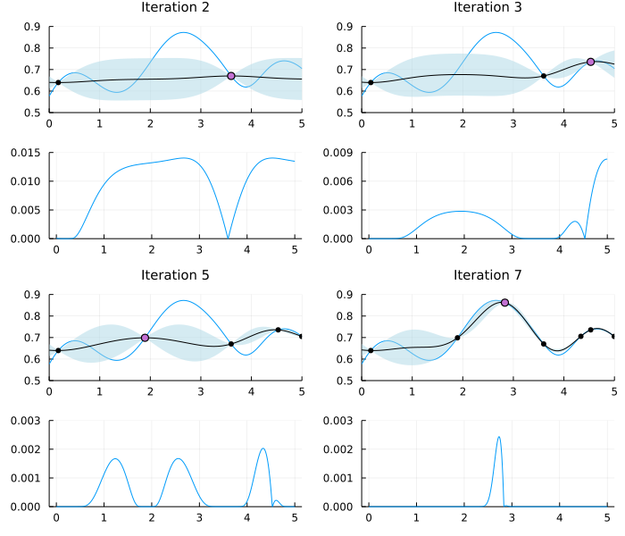
The exploitation-exploration trade-off is illustrated in Figure 2, where the blue line shows the true objective function, the black line denotes the posterior mean of the GP, and the blue-shaded regions are 95% posterior probability bands for $f$. The black (small) dots are past function evaluations, and the violet (large) dot is the current evaluation. The first and third row in Figure 2 show the true objective function and the learned GP at four different iterations of the algorithm while the second and fourth row show the EI acquisition function corresponding to the row immediately above. At Iteration 2 in the top-left corner, we see that the EI acquisition function (second row) indicates that there is a high expected improvement by moving to either the immediate left or right of the current evaluation. At Iteration 5 the EI strategy suggests three regions worth evaluating, where the two leftmost regions are candidates because of their high uncertainty. After seven iterations, the algorithm is close to the global maximum and will now continue a narrow search for the exact location of the global maximum.

Acquisition rules like PI or EI do not consider that different evaluation points can be more or less costly. To introduce the notation of cost into the acquisition strategy, Snoek et al., (2012) proposed Expected Improvement per second, $\text{EIS}(\mathbf{x})\equiv\text{EI}(\mathbf{x})/c(\mathbf{x})$, where $c:\mathcal{X}\to\mathbb{R}^{+}$ is a duration function that measures the evaluation time at input $\mathbf{x}$ in seconds. More generally, we can define $a(\mathbf{x})/c(\mathbf{x})$ as an effort-aware acquisition function. The duration function is typically unknown and Snoek et al., (2012) proposed to estimate it alongside $f$ using an additional Gaussian process for $\log c(\mathbf{x})$.

EIS assumes that the duration (or the cost) of function evaluations are unknown, but fixed for a given input $\mathbf{x}$; once we visit $\mathbf{x}$, the cost of the function estimate $\hat{f}(\mathbf{x})$ is given. However, the user can often choose the duration spent to obtain a certain precision in the estimate; for example by increasing the number of MCMC iterations when the marginal likelihood is estimated by MCMC. This novel perspective opens up for strategies that not only optimize for the next evaluation point, but also optimize over the computational resources, or equivalently, the precision of the estimate $\hat{f}(\mathbf{x})$. We formally extend BO by modeling the function evaluations with a heteroscedastic GP

where the noise variance $\sigma^{2}(\mathbf{x},G)$ is now an explicit function of the number of MCMC iterations, $G$, or some other duration measure. Hence the user can now choose both where to place the next evaluation and the effort spent in computing it by maximizing

with respect to both $\mathbf{x}$ and $G$, where $a(\mathbf{x})$ is a baseline acquisition function, for example EI.

A complication with maximization of $\tilde{a}(\mathbf{x},G)$ is that while we typically know that $\sigma(\mathbf{x},G)=O(1/\sqrt{G})$ in Monte Carlo or MCMC, the exact numerical standard error depends on the integrated autocorrelation time (IACT) of the MCMC chain. Note that the evaluation points can, for example, be hyperparameters in the prior, where different values can give rise to varying degrees of well-behaved posteriors, so we can not expect the IACT to be constant over the hyperparameter space, hence the explicit dependence on $\boldsymbol{x}$ in $\sigma^{2}(\mathbf{x},G)$. Rather than maximizing $\tilde{a}(\mathbf{x},G)$ with respect to both $\mathbf{x}$ and $G$ directly, we propose to implement the algorithm in an alternative way that achieves a similar effect. The approach includes stopping the evaluation early whenever the function evaluation turns out to be hopelessly low with a low probability of improvement over the current $f_{max}$.

For a given $\mathbf{x}$ we let $G$ increase, in batches of a fixed size, until

for some small value, $\alpha$, or until $G$ reaches a predetermined upper bound, $\bar{G}$; here $\hat{m}^{(g)}(\mathbf{x})\text{ and }s^{(g)}(\mathbf{x})$ denotes the posterior mean and standard deviation of the GP evaluated at $\mathbf{x}$ after $g$ MCMC iterations. Note that both the posterior mean $m(\mathbf{x})$ and standard deviation $s(\mathbf{x})$ are functions of the noise variance, which in turn is a function of $G$. The posterior distribution for $f(\mathbf{x})$ is hence continuously updated as $G$ grows until $1-\alpha$ of the posterior mass in the GP for $f(\mathbf{x})$ is concentrated below $f_{max}$, at which point the evaluation stops. The optimization is insensitive to the choice of $\alpha$, as long as it is a relatively small number. We now propose to maximize the following acquisition function based on early stopping

where $\hat{G}_{\alpha}(\mathbf{x})$ is a prediction of the number of MCMC draws needed at $\mathbf{x}$ before the evaluation stops, with the probability $\alpha$ as the threshold for stopping. We emphasize that early stopping is here used in a subtle way, not only as a simple rule to short-circuit useless computations, but also in the planning of future computations; the mere possibility of early stopping can make the algorithm try an $\mathbf{x}$ which does not have the highest $a(\mathbf{x})$, but which is expected to be cheap and is therefore worth a try. This effect that comes via $\sigma^{2}(G)$ is not present in the EIS of Snoek et al., (2012) where the cost is fixed and is not influenced by the probability model on $f$.

Although one can use any model to predict $G$, we will here fit a GP regression model to the logarithm of the number of MCMC draws, $\log G_{j}$ for $j=1,...,J$ in the $J$ previous evaluations

where $\mathbf{z}_{j}$ is a vector of covariates. The hyperparameters, $\mathbf{x}_{1:J}$, themselves may be used as predictors of $\hat{G}(\mathbf{x})$, but also $D(\mathbf{x})=\hat{m}(\mathbf{x})-f_{max}$ and $s(\mathbf{x})$ are likely to have predictive power for $G$, as well as $u(\mathbf{x})=(\hat{m}(\mathbf{x})-f_{max})/s(\mathbf{x})$. We will use $\mathbf{z}_{j}=\left(\mathbf{x}_{j},D^{(j)}(\mathbf{x}_{j}),s^{(j)}(\mathbf{x}_{j}),u^{(j)}(\mathbf{x}_{j})\right)$ in our applications, where the superscript over $j$ denotes the BO iteration. The prediction for $G$ is taken to be $\hat{G}=\text{exp}\left(m_{G}\left(\mathbf{z}\right)\right)$, which corresponds to the median of the log-normal posterior for $G$.

We will use the term Bayesian Optimization with Optimized Precision (BOOP) for BO methods that optimize $\tilde{a}_{\alpha}(\mathbf{x})$ in (16), and more specifically BOOP-EI when EI is used as the baseline acquisition function, $a(\mathbf{x})$. The whole procedure is described in Algorithm 1.

Note that (13) assumes that $\hat{f}(\mathbf{x})$ is an unbiased estimator at any $\mathbf{x}$. This can be ensured by using enough MCMC/importance sampling draws in the first marginal likelihood evaluation of BOOP. We performed a small simulation exercise that shows that the Chib estimator is approximately unbiased after a small number of iterations for the medium-sized VAR model in 5.4. As expected, we had to use more initial draws in the large-scale VAR in Section 5.5 and the time-varying parameter VAR with stochastic volatility in Section 6 to drive down the bias. See also Section 7 for some ideas on how to extend BOOP to estimators where the bias is still sizeable in large MCMC samples.

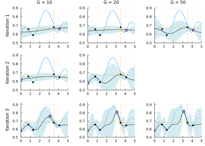
Figure 3 illustrates the early stopping part of BOOP in a toy example. The first row illustrates the first BOOP iteration and the columns show increasingly larger MCMC sample sizes ($G$). We can see that the 95% posterior interval after $G=10$ MCMC draws at the current $\mathbf{x}$ includes $f_{max}^{(1)}$ (dotted orange line), the highest posterior mean of the function values observed so far; it therefore worthwhile to increase the number of simulations for this $\mathbf{x}$. Moving one graph to the right we see that after $G=20$ simulations the 95% posterior interval still includes $f_{max}^{(1)}$, and we move one more graph to the right for $G=50$. Here we conclude that the sampled point is almost certainly not an improvement and we move on to a new evaluation point. The new evaluation point is found by maximizing the BOOP-EI acquisition function in (16) with updated effort prediction function $\hat{G}(\boldsymbol{z})$ in Equation 17 and is depicted by the violet dot in leftmost graph in the second row of Figure 3. Following the progress in the second row, we see that it takes only $G=20$ samples to conclude that the function value is almost certainly lower than the current maximum of the posterior mean at the second BO iteration. Finally, in the third row, we can see that the point is sampled with high variance at the beginning, but as we increase $G$ it becomes clear that this $\mathbf{x}$ is indeed an improvement.

The code used in this paper is written in the Julia computing language (Bezanson et al.,, 2017), making use of the GaussianProcesses.jl package for estimation of the Gaussian processes and the Optim.jl package for the optimization of the acquisition functions.

We will here assess the performance of the proposed BOOP-EI algorithm in a simulation experiment for the optimization of a non-linear function in a single variable. The simple one-dimensional setup is chosen for presentational purposes, and more challenging higher-dimensional settings are likely to show even larger advantages of our method compared to regular Bayesian optimization.

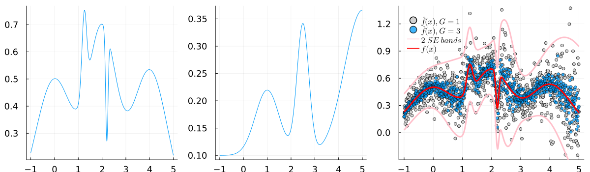
The function to be maximized is

where $N(x|\mu,\sigma^{2})$ denotes the density function of a $N(\mu,\sigma^{2})$ variable; the function is plotted in Figure 4 (left). We further assume that $f(x)$ can be estimated at any $x$ from $G$ noisy evaluations by a simple Monte Carlo average

where $g(x)=0.1+0.15N(x|1,0.5^{2})+0.15N(x|2.5,0.25^{2})+0.5N(x|5,0.75^{2})$ is a heteroscedastic standard deviation function that mimics the real world case where the variability of the marginal likelihood estimate varies over the space of hyperparameters; $g(x)$ is plotted in Figure 4 (middle). Figure 4 (right) illustrates the noisy function evaluations (gray points) and the effect of Monte Carlo averaging $G=3$ evaluations for a given $x$ (blue points). We assume for simplicity here that once the algorithm decides to visit an $x$ it will get access to a noise-free evaluation of the standard error of the estimator.

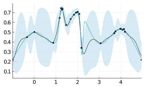
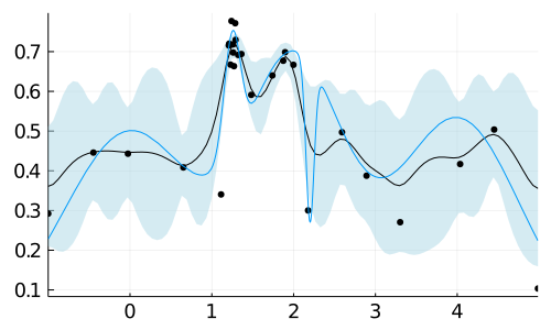
Before we conduct a small Monte Carlo experiment it is illustrative to look at the results from a single run of the EI and BOOP-EI algorithms. Figure 5 highlights the difference between the algorithms by showing the GP posterior after 25 Bayesian optimization runs. The EI algorithm has clearly wasted computations to needlessly drive down the uncertainty at (useless) low function values, while BOOP-EI tolerates larger uncertainty in such function locations.

We now compare the performance of a standard EI approach using a heteroscedastic GP with our BOOP-EI approach in a small simulation study. The methods will be judged by their ability to find the optimum using as few evaluations as possible. The performance will be evaluated by a Monte Carlo study where we simulate $1000$ replications from each model under each simulation scenario. We investigate Bayesian optimization with EI using $100$ and $500$ samples in each iteration, BOOP-EI is allowed to stop the sampling at any time before the number of samples for the EI is reached. In each simulation we set an upper bound of $120$ Bayesian optimization iterations.

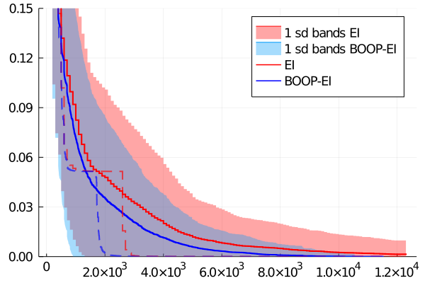
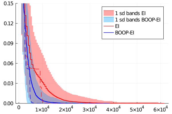
We can see from Figure 6 that BOOP finds the maximum by using fewer total number of samples in both scenarios and that the difference increases with the number of samples used when forming the estimator. We can also see from the median $f_{max}$ that both algorithms can get stuck for a while at the second greatest local maximum (which is approximately $.05$ lower than the global maximum). However, BOOP gets out of the local optimum faster since it has the option to try cheap noisy evaluations and will therefore explore other parts of the function earlier than basic BO-EI. This effect seems to increase as we allow for a higher number of samples since it lowers the relative price of cheaper evaluations.

The steady-state BVAR model of Villani, (2009) is given by:

where $E[\mathbf{y}_{t}]=\Psi\mathbf{x}_{t}$. In particular, if we assume that $\mathbf{x}_{t}=1$ for all $t,$ then $\Psi$ has the interpretation as the overall mean of the process. We take the prior distribution to be:

where $\underline{\boldsymbol{\theta}}_{\Psi}\text{ and }\underline{\Omega}_{\Psi}$ are the mean and covariance matrix for the steady states. The prior covariance matrix for the dynamics, $\underline{\Omega}_{\Pi}$, is constructed using

where $\underline{\omega}_{ii}$ is the diagonal elements of $\underline{\Omega}_{\Pi}$. We also assume prior independence, following Villani, (2009). The hyperparameters that we optimize over are: the overall-shrinkage parameter $\theta_{1}$, the cross-lag shrinkage $\theta_{2}$, and the lag-decay parameter $\theta_{3}$.

The posterior distribution of the steady-state BVAR model parameters can be sampled with a simple Gibbs sampling scheme (Villani,, 2009). The marginal likelihood, together with its empirical standard error, can be estimated by the method in Chib, (1995).

Table 1 describes the data used in our applications which are also used in Giannone et al., (2015). It contains 23 macroeconomic variables for which two subsets are selected to represent a medium-sized model with 7 variables and a large model that contains 22 of the variables (real investment is excluded). Before the analysis, the consumer price index and the five-year bond rate were transformed from monthly to quarterly frequency. All series are transformed such that they become stationary according to the augmented Dickey-Fuller test. This is necessary for the data to be consistent with the prior assumption of a steady-state. The number of lags is chosen according to the HQ-criteria, Hannan and Quinn, (1979) and Quinn, (1980). This resulted in $p=2$ lags for the medium-sized model which we also use for the large model.

We set the prior mean of the coefficient matrix, $\Pi$, to values that reflect some persistence on the first lag, but also that all the time series are stationary; e.g. the prior mean on the first lag of the FED interest rate and the GDP-deflator is set to 0.6, while others are set to zero in the medium-sized model. Lags longer than 1 and cross-lags all have zero prior means. The priors for the steady-states are set informative to the values listed in Table 1, these values follow suggestions from the literature for most variables, see e.g. Louzis, (2019) and Österholm, (2012). There were a few variables where we could not find theoretical values for either the mean or the standard deviation, in those cases, we set them close to their empirical counterparts.

We consider three competing optimization strategies: (I) an exhaustive grid-search, (II) Bayesian optimization with the EI acquisition function (BO-EI), and (III) our BOOP-EI algorithm. In each approach, we use the restrictions $\theta_{1}\in(0,5),\theta_{2}\in(0,1)\text{, and }\theta_{3}\in(0,5)$. In the grid-search, $\theta_{1}\text{ and }\theta_{2}$ move in steps of $0.05$ and $\theta_{3}$ moves in steps of $0.1$, yielding in total 100000 marginal likelihood evaluations. For the Bayesian optimization algorithm, we set the number of evaluations to 250, and we use three random draws as initial values for the GPs.

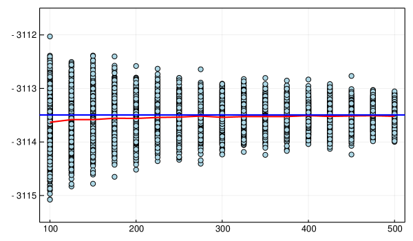
For strategies (I) and (II) we use a total of 10000 Gibbs iterations with 1000 as a burn-in sample in each model evaluation. For (III) we first draw 1100 Gibbs samples where we discard the first 1000 as burn-in and use the rest to calculate the probability of improvement PI, to ensure that the estimated marginal likelihood will be approximately unbiased; Figure 7 shows that Chib’s estimate is unbiased already after a few hundred samples. If $\text{PI}<\alpha$ we stop early and move on to the next BO iteration, otherwise we generate a new batch (of size 100) of Gibbs samples and again check the PI criteria. The total number of Gibbs iterations will therefore vary between 1100 and 10 000 in each of the 250 BOOP-iterations for the medium-sized model. Note that Chib’s estimator uses an estimate of the parameter for the so-called reduced Gibbs sampler run. This point estimate should preferably have a high posterior density for efficiency reasons, see Chib, (1995). The medium-sized model uses only 100 posterior samples to obtain high-density parameters for calculating Chib’s log marginal likelihood, which is enough in our set-up. For the large model, we use $5000$ burn-in samples and $500$ simulations in the first batch, which gives between $5500$ and $10000$ MCMC iterations per evaluation point. The $5000$ burn-in is likely to be excessive but is used to be conservative; a small number would make BOOP even faster in comparison to regular BO. The application is robust to the choice of $\alpha$, as long as it is a reasonably low number, in this study we use $\alpha=0.001$.

For comparison, we will also use the standard values of the hyperparameters used in e.g. the BEAR-toolbox, Dieppe et al., (2016), $\theta_{1}=0.1,\theta_{2}=0.5,\text{ and }\theta_{3}=1$, as a benchmark. The methods are compared with respect to i) the obtained marginal likelihood, and ii) how much computational resources were spent in the optimization.

Table 2 summarizes the results from ten runs of the algorithms for the medium size BVAR model. We see that all three optimization strategies find hyperparameters that yield substantially higher log marginal likelihood than the standard values. We can also see that both Bayesian optimization methods yield as good hyperparameters as the grid search at only a small fraction of the computational cost. It is also clear from Table 2 that a substantial amount of computations associated with the MCMC are saved when using BOOP. It is interesting to note that the values for $\theta_{1}\text{ and }\theta_{2}$ are similar for all three optimization approaches but that $\theta_{3}$ differs to some extent. This is due to the flatness of the log marginal likelihood in that area.

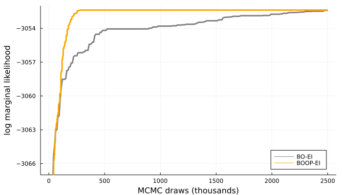
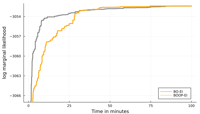
The left graph of Figure 8 shows that BOOP-EI finds higher values of the log marginal likelihood using much fewer MCMC iterations than plain BO with EI acquisitions. From Table 2 we can see that BOOP-EI uses, on average, less than a fifth of the MCMC iterations compared to BO-EI for a full run. Interesting to note is that BO-EI leads to (on average) a higher number of improvements on the way to the maximum; while BOOP-EI gives fewer improvements but of larger magnitude; the strategy of cheaply exploring new territories before locally optimizing the function pays off. The graph to the right in Figure 8 shows that for this application BO-EI is quicker in terms of CPU time to reach fairly high values for the log marginal likelihood. We see at least two explanations for this: first, BOOP-EI tries to explore more unknown territories since they are presumed to be cheap while BO-EI more greedily focuses on local optimization. Second, and more importantly, the overhead cost associated with the BOOP-EI acquisition is relatively large in this medium-sized application where the cost of evaluating the marginal likelihood itself is not excessive. The fact that BOOP can heavily reduce the number of MCMC draws while still giving similar CPU computational time suggest that it is most useful in cases where each log marginal likelihood evaluation is expensive; this will be demonstrated in the more computationally demanding models in Sections 5.5 and 6.

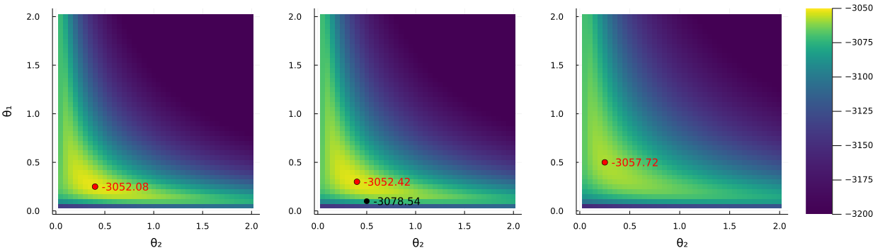
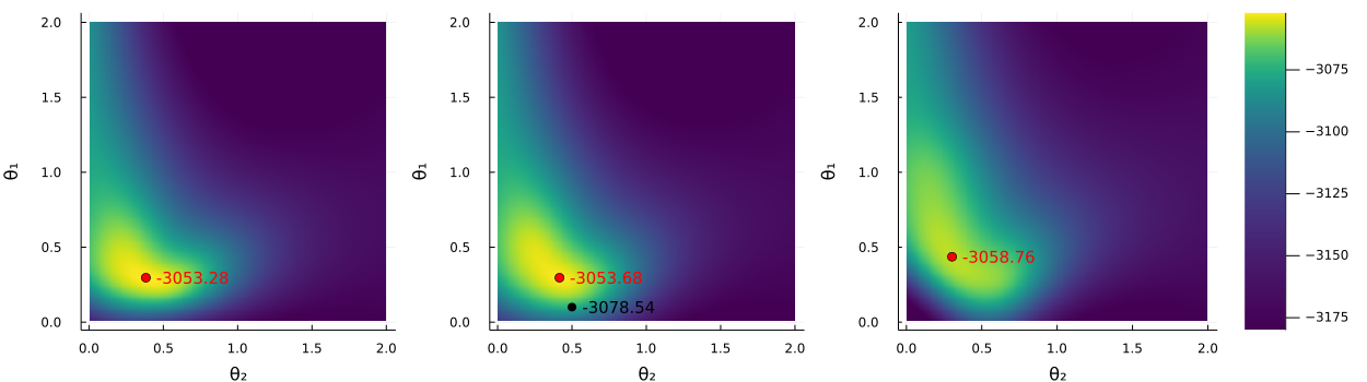
Figure 9 displays the log marginal likelihood surfaces over the grid of $(\theta_{1},\theta_{2})$-values used in the grid search. Each sub-graph is for a fixed value of $\theta_{3}\in\{0.76,1,2\}$. The red dot indicates the predicted maximum log marginal likelihood for the given $\theta_{3},$ and the black dot in the middle sub-figure indicates the standard values. We can see that the standard values are located outside the high-density region, relatively far away from the maximum. A comparison of Figures 9 and 10 shows that the GP’s predicted log marginal likelihood surface is quite accurate already after merely 250 evaluations; this is quite impressive considering that Bayesian optimization tries to find the maximum in the fastest way, and does not aim to have high precision in low-density regions.

We also optimize the parameters of the more challenging large BVAR model containing the 22 different time series, using 250 iterations for both BO-EI and BOOP-EI. A complete grid search is too costly here, so we instead compare with parameters obtained from BOOP in the medium-sized BVAR in Section 5.4, which is a realistic strategy in practical work.

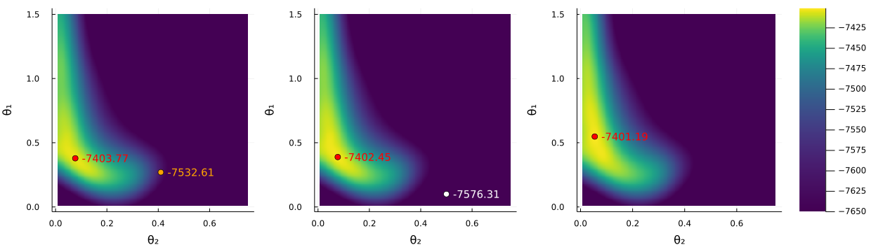
Table 3 shows that our method, again, finds optimal hyperparameters with dramatically larger log ML than standard values, and also substantially better values than those that are optimal for the medium-scale BVAR. Finally, note that the hyperparameters selected by BOOP-EI in the large-scale BVAR are quite different from those in the medium-scale model. The optimal $\theta_{1}$ applies less baseline shrinkage than before, but the lag decay ($\theta_{3}$) is higher, and in particular, the cross-lag shrinkage, $\theta_{2}$, is much closer to zero, implying much harder shrinkage towards univariate AR-processes. This latter result strongly suggests that the computationally attractive conjugate prior structure is a highly sub-optimal solution since such a prior requires that $\theta_{2}=1$. We can see that for this more computationally demanding model BOOP-EI is much faster and finish on average in a third of the time than the regular BO-EI strategy. Figure 11 show the predicted log marginal likelihood surface obtained from the last GP in a BOOP run. The rightmost graph conditions on $\theta_{3}=1.51$, which is optimal for BOOP-EI, so this graph therefore has the GP with the highest accuracy.

The time-varying parameter BVAR with stochastic volatility (TVP-SV BVAR) in Chan and Eisenstat, (2018) is given by

where $\boldsymbol{\mu}_{t}$ is a vector of time varying intercepts, $\boldsymbol{B}_{1t},\dots,\boldsymbol{B}_{pt}$ are $n\times n$ matrices of VAR coefficients, $\boldsymbol{B}_{0t}$ is a $n\times n$ lower triangular matrix with ones on the main diagonal. The evolution of $\boldsymbol{\Sigma}_{t}=\mathrm{diag}\left(\exp(h_{1t}),\dots,\exp(h_{nt})\right)$ is modelled by the vector of log volatilities, $\mathbf{h}_{t}=(h_{1t},\dots,h_{nt})^{\top}$, evolving as a random walk

where $\boldsymbol{\Sigma}_{h}=\mathrm{diag}(\sigma_{h_{1}}^{2},\dots,\sigma_{h_{n}}^{2})$ and the starting values in $\mathbf{h}_{0}$ are parameters to be estimated. Following Chan and Eisenstat, (2018), we collect all parameters of $\boldsymbol{\mu}_{t}$ and the $\mathbf{B}_{it}$ matrices in a $k_{\gamma}$-dimensional vector $\boldsymbol{\gamma}_{t}$ and write the model in state space form as

where $\boldsymbol{X}_{t}$ contain both current and lagged values of $\mathbf{y}$, $\boldsymbol{\Sigma}_{\gamma}=\mathrm{diag}(\sigma_{\gamma_{1}}^{2},\dots,\sigma_{\gamma_{k\gamma}}^{2})$ and the initial values for the state variables follow $\boldsymbol{\boldsymbol{\gamma}}_{0}\sim N(\mathbf{a}_{\boldsymbol{\gamma}},\mathbf{V}_{\boldsymbol{\gamma}})$ and $\mathbf{h}_{0}\sim N(\mathbf{a}_{\mathbf{h}},\mathbf{V}_{\mathbf{h}})$.

For comparability we choose to use the same prior setup as in Chan and Eisenstat, (2018) where the variances of the state innovations follow independent inverse-gamma distributions: $\sigma_{\gamma_{i}}^{2}\sim IG(\nu_{\gamma_{0}},S_{\gamma_{0}})$ if $\gamma_{i}$ is an intercept, $\sigma_{\gamma_{i}}^{2}\sim IG(\nu_{\gamma_{1}},S_{\gamma_{1}})$ if $\gamma_{i}$ is a VAR coefficient and $\sigma_{h}^{2}\sim IG(\nu_{h},S_{h})$ for the innovations to the log variances. Following Chan and Eisenstat, (2018) we set $\mathbf{a}_{\boldsymbol{\gamma}}=\boldsymbol{0}$, $\mathbf{V}_{\boldsymbol{\gamma}}=10\cdot I_{k_{\gamma}}$, $\mathbf{a}_{\mathbf{h}}=0$, $\mathbf{V}_{\mathbf{h}}=10\cdot I_{n}$, and $\nu_{\gamma_{0}}=\nu_{\gamma_{1}}=\nu_{h}=5$, but we use Bayesian optimization to find the optimal values for the three key hyperparameters $S_{\gamma_{0}}$, $S_{\gamma_{1}}$ and $S_{h}$ which controls the degree of time-variation in the states. We collect the three optimized hyperparameter in the vector $\boldsymbol{\theta}=(\theta_{1},\theta_{2},\theta_{3})^{\top}$, where $\theta_{1}=S_{\gamma_{0}}$, $\theta_{2}=S_{\gamma_{1}}$ and $\theta_{3}=S_{h}$. We optimize over the domain $\{\boldsymbol{\theta}:0\leq\theta_{1}\leq 5,0\leq\theta_{2}\leq 1,0\leq\theta_{3}\leq 5\}$, which allows for all cases from no time variation in any parameter to high time variation in all the model parameters.

To estimate the marginal likelihood, Chan and Eisenstat, (2018) first obtain posterior draws of $\boldsymbol{\gamma},\boldsymbol{h},\Sigma_{\boldsymbol{\gamma}},\Sigma_{\mathbf{h}},\boldsymbol{\gamma}_{0},\mathbf{h}_{0}$ using Gibbs sampling, which are then used to design efficient importance sampling proposals. The marginal likelihood is

where $\boldsymbol{\psi}$ collects all the static parameters in $\Sigma_{\boldsymbol{\gamma}},\Sigma_{\mathbf{h}},\boldsymbol{\gamma}_{0},\mathbf{h}_{0}$. The inner integral w.r.t. $\boldsymbol{\gamma}$ can be solved analytically and afterwards, we can integrate out $\mathbf{h}$ using importance sampling to obtain an estimate of the integrated likelihood

The last step is to integrate out the fixed parameters from the integrated likelihood

which is done using another importance sampler. The two nested importance samplers put the algorithm in the framework of importance sampling squared ($IS^{2}$, Tran et al., (2013)). The Chan-Eisenstat algorithm is elegantly designed, but necessarily computationally expensive with a single estimate of the marginal likelihood taking 205 minutes in MATLAB on a standard desktop (Chan and Eisenstat,, 2018). We call their MATLAB code from Julia using the MATLAB.jl package, illustrating that BOOP can plug in any marginal likelihood estimator. However, we found that the standard errors in Chan and Eisenstat, (2018) can be more robustly estimated using the bootstrap and we have done so here. The cost of bootstrapping the standard errors only has to be taken once for every Bayesian optimization iteration, and this cost is negligible compared to the computation of the log marginal likelihood estimate.

We use quarterly data for the GDP-deflator, real GDP, and the short-term interest rate in the USA from 1954Q3 to 2014Q4 from Chan and Eisenstat, (2018) for comparability. In addition, we make use of their Matlab code (with minor adjustments) for computing the marginal likelihood. This shows another strength with the BOOP approach, that it works on top of existing code.

We fix the number of Gibbs sampling iterations and the burn-in period to $20000$ and $5000$ respectively for both BO-EI and BOOP-EI in all evaluation points. This simplifies the implementation and does not make a practical difference since the main part of the computational cost is spent on the log marginal likelihood estimate from importance sampling. For BO-EI we use $5000$ log marginal likelihood evaluations in each new evaluation point, while BOOP-EI starts with $1000$ importance sampling draw and then takes batches of size $100$ until a maximum of $5000$ samples has been reached. The initial 1000 draws were enough to make the estimator approximately unbiased.

Table 4 shows the optimized log marginal likelihood from three independent runs of BO-EI and BOOP-EI; the hyperparameter values used in Chan and Eisenstat, (2018) are shown for reference. As expected both BO and BOOP find better hyperparameters than the ones in Chan and Eisenstat, (2018); this is particularly true for BOOP which gives an increase in the marginal likelihood of more than 10 units on the log scale on average. Interestingly, both BO and BOOP suggest that the stochastic volatilities should be allowed to move more freely than in Chan and Eisenstat, (2018), but that there should be less time variation in the intercepts and VAR coefficients. This points in the same direction as the results in Chan and Eisenstat, (2018) who find that shutting down the time variation in the intercept and VAR coefficients actually increases the marginal likelihood. Our results indicate that when carefully selecting the shrinkage parameters by optimization, the VAR-dynamics should in fact be allowed to evolve over time, but at a slower pace.

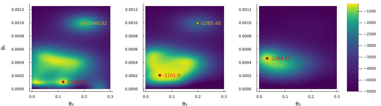
Table 4 shows a great deal of variability between runs, in particular for BO. Figure 12 shows that this is probably because the hyperparameter surface is substantially more complicated and multimodal than for the steady-state BVAR. We can also see that the log marginal likelihood is relatively insensitive to changes in $\theta_{3}$ around the mode while it is very sensitive to changes in $\theta_{2}$.

References

- Adolfson et al., (2007) Adolfson, M., Lindé, J., and Villani, M. (2007). Bayesian analysis of DSGE models-some comments. Econometric Reviews, 26(2-4):173–185.
- An and Schorfheide, (2007) An, S. and Schorfheide, F. (2007). Bayesian analysis of DSGE models. Econometric reviews, 26(2-4):113–172.
- Bańbura et al., (2010) Bańbura, M., Giannone, D., and Reichlin, L. (2010). Large Bayesian vector auto regressions. Journal of Applied Econometrics, 25(1):71–92.
- Bezanson et al., (2017) Bezanson, J., Edelman, A., Karpinski, S., and Shah, V. B. (2017). Julia: A fresh approach to numerical computing. SIAM review, 59(1):65–98.
- Brochu et al., (2010) Brochu, E., Cora, V. M., and De Freitas, N. (2010). A tutorial on Bayesian optimization of expensive cost functions, with application to active user modeling and hierarchical reinforcement learning. arXiv preprint arXiv:1012.2599.
- Carriero et al., (2012) Carriero, A., Kapetanios, G., and Marcellino, M. (2012). Forecasting government bond yields with large Bayesian vector autoregressions. Journal of Banking & Finance, 36(7):2026–2047.
- Chan and Eisenstat, (2018) Chan, J. C. and Eisenstat, E. (2018). Bayesian model comparison for time-varying parameter vars with stochastic volatility. Journal of applied econometrics, 33(4):509–532.
- Chib, (1995) Chib, S. (1995). Marginal likelihood from the Gibbs output. Journal of the American Statistical Association, 90(432):1313–1321.
- Chib and Jeliazkov, (2001) Chib, S. and Jeliazkov, I. (2001). Marginal likelihood from the Metropolis-Hastings output. Journal of the American Statistical Association, 96(453):270–281.
- Dieppe et al., (2016) Dieppe, A., Legrand, R., and Van Roye, B. (2016). The BEAR toolbox.
- Doan et al., (1984) Doan, T., Litterman, R., and Sims, C. (1984). Forecasting and conditional projection using realistic prior distributions. Econometric reviews, 3(1):1–100.
- Doucet et al., (2001) Doucet, A., De Freitas, N., Gordon, N. J., et al. (2001). Sequential Monte Carlo methods in practice. Springer.
- Geweke, (1999) Geweke, J. (1999). Using simulation methods for Bayesian econometric models: inference, development, and communication. Econometric reviews, 18(1):1–73.
- Geweke and Keane, (2007) Geweke, J. and Keane, M. (2007). Smoothly mixing regressions. Journal of Econometrics, 138(1):252–290.
- Giannone et al., (2015) Giannone, D., Lenza, M., and Primiceri, G. E. (2015). Prior selection for vector autoregressions. Review of Economics and Statistics, 97(2):436–451.
- Hannan and Quinn, (1979) Hannan, E. J. and Quinn, B. G. (1979). The determination of the order of an autoregression. Journal of the Royal Statistical Society: Series B (Methodological), 41(2):190–195.
- Karlsson, (2013) Karlsson, S. (2013). Forecasting with Bayesian vector autoregression. In Handbook of Economic Forecasting, volume 2, pages 791–897. Elsevier.
- Louzis, (2019) Louzis, D. P. (2019). Steady-state modeling and macroeconomic forecasting quality. Journal of Applied Econometrics, 34(2):285–314.
- Matérn, (1960) Matérn, B. (1960). Spatial variation. Medd. fr. St. Skogsf. Inst. 49 (5). Reprinted in Lecture Notes in Statistics no. 36.
- Österholm, (2012) Österholm, P. (2012). The limited usefulness of macroeconomic Bayesian VARs when estimating the probability of a US recession. Journal of Macroeconomics, 34(1):76–86.
- Primiceri, (2005) Primiceri, G. E. (2005). Time varying structural vector autoregressions and monetary policy. The Review of Economic Studies, 72(3):821–852.
- Quinn, (1980) Quinn, B. G. (1980). Order determination for a multivariate autoregression. Journal of the Royal Statistical Society: Series B (Methodological), 42(2):182–185.
- Snoek et al., (2012) Snoek, J., Larochelle, H., and Adams, R. P. (2012). Practical bayesian optimization of machine learning algorithms. In Advances in neural information processing systems, pages 2951–2959.
- Tran et al., (2013) Tran, M.-N., Scharth, M., Pitt, M. K., and Kohn, R. (2013). Importance sampling squared for bayesian inference in latent variable models. arXiv preprint arXiv:1309.3339.
- Villani, (2009) Villani, M. (2009). Steady-state priors for vector autoregressions. Journal of Applied Econometrics, 24(4):630–650.
- Villani et al., (2012) Villani, M., Kohn, R., and Nott, D. J. (2012). Generalized smooth finite mixtures. Journal of Econometrics, 171(2):121–133.
- Williams and Rasmussen, (2006) Williams, C. K. and Rasmussen, C. E. (2006). Gaussian processes for machine learning, volume 2. MIT Press Cambridge, MA.