¹¹institutetext: Indian Association for the cultivation of Science
¹¹email: tpab2@iacs.res.in,
home page: http://inspirehep.net/author/profile/Arita.Biswas.1

$b\to cl\nu$ anomalies in light of vector and scalar interactions

Aritra Biswas 11

Abstract

We perform a model independent analysis of the charged current $b\to cl\nu$ anomalies under the presence of scalar and vector interactions. The analysis is carried out in two stages: (a) under the presence of both (left-handed) vector and scalar interactions and (b) under the presence of scalar interactions alone. We find that even after stringent bounds from similar quark-level processes such as $B_{c}\to\tau\nu$ , such scenarios have the potential to explain the aforementioned anomalies. Contrary to the general notion, we show that even scalar interactions alone can explain such anomalies, provided they are complex. However, extended scalar sector models are unable to comply with these anomalies to $\sim 3\sigma$ . We further illustrate our results with the help of three benchmark models corresponding to the presence of (i) both scalar and vector (ii) real scalar and (iii) complex scalar interactions.

keywords:

Flavour Physics, Mesons, Hadrons

1 Introduction

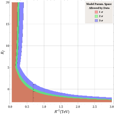
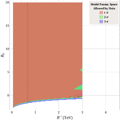
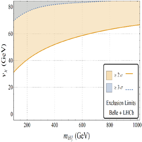
Over the past few years, there have been constant and consistent reports from experimental collaborations such as LHCb, Belle and BaBar about flavour observables with deviations of more than $3\sigma$ in exclusive $B\to D^{*}$ [1, 2, 3, 4, 5, 6, 7, 8, 9] and $B\to J/\psi$ transitions. Both of these exclusive processes have the underlying sub-quark transition $b\to cl\nu$ . These results are believed to be the hints of lepton-flavour universality violating (LFUV) type new physics (NP). We investigate the prospect of scalar and vector type NP’s in explaining such deviations. We initially work from a model independent perspective and then illustrate our results further using the models: (i) Non-minimal universal extra dimensions (NMUED) for the case with one scalar and one vector NP operator, (ii) Goergi-Michacek (GM) model for the case of a single scalar NP operator preceded by a real Wilson coefficient (WC) and (iii) Leptoquark (LQ) model for the a single scalar NP operator preceded by a complex WC.

2 Current Status: Theory and Experiment

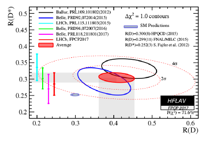
The present global average for the $\mathcal{R}(D^{(*)})$ anomalies are about $4\sigma$ away from the corresponding SM results. Fig. 5 and table. 1 summarize the current theoretical and experimental status for these anomalies. The SM average is the arithmetic mean of the results from [10, 11, 12, 13].

	$\mathcal{R}(D)$	$\mathcal{R}(D^{*})$	Correlation	$P_{\tau}(D^{*})$	$\mathcal{R}(J/\psi)$
SM	$0.299(3)$	$0.258(6)$		$-0.491(25)$	$0.249(42)$ (LFCQ)
					$0.289(28)$ (PQCD)
Babar	$0.440(58)_{st.}(42)_{sy.}$	$0.332(24)_{st.}(18)_{sy.}$	$-0.27$
Belle (2015)	$0.375(64)_{st.}(26)_{sy.}$	$0.293(38)_{st.}(15)_{sy.}$	$-0.49$
Belle (2016)-I	-	$0.302(30)_{st.}(11)_{sy.}$
Belle (2016)-II	-	$0.270(35)_{st.}~^{+0.028}{}_{-0.025}$	0.33	$-0.38(51)_{st.}~^{+0.21}{}_{-0.16}$
LHCb (2015)	-	$0.336(27)_{st.}(30)_{sy.}$
LHCb (2017)	-	$0.286(19)_{st.}(25)_{sy.}(21)$
World Avg.	$0.407(39)_{st.}(24)_{sy.}$	$0.304(13)_{st.}(7)_{sy.}$	$0.20$		$0.71(17)_{st.}(18)_{sy.}$

Table 1: Present status (both theoretical and experimental) of

\mathcal{R}(D)

\mathcal{R}(D^{*})

and

P_{\tau}(D^{*})

. First uncertainty is statistical and the second one is systematic. The first row lists the arithmetic mean for the SM calculations reported in HFLAV.

Refer to caption — Figure 1: Global average for $\mathcal{R}(D)$ , $\mathcal{R}(D^{*})$ and $P_{\tau}(D^{*})$ and the deviation from the SM result.

3 Formalism

The most general effective Hamiltonian describing the $b\to c\tau\nu$ transitions, with all possible four-fermi operators in the lowest dimension (with left-handed neutrinos) is given by:

{\cal H}_{eff}=\frac{4G_{F}}{\sqrt{2}}V_{cb}\Big{[}(1+C^{\ell}_{V_{1}}){\cal O}_{V_{1}}+C^{\ell}_{V_{2}}{\cal O}_{V_{2}}+C^{\ell}_{S_{1}}{\cal O}_{S_{1}}+C^{\ell}_{S_{2}}{\cal O}_{S_{2}}+C^{\ell}_{T}{\cal O}_{T}\Big{]},

(1)

where the operator basis is defined as

$\displaystyle{\cal O}_{V_{1}}$	$\displaystyle=$	$\displaystyle({\bar{c}}_{L}\gamma^{\mu}b_{L})({\bar{\tau}}_{L}\gamma_{\mu}\nu_{\tau L}),$
$\displaystyle{\cal O}_{V_{2}}$	$\displaystyle=$	$\displaystyle({\bar{c}}_{R}\gamma^{\mu}b_{R})({\bar{\tau}}_{L}\gamma_{\mu}\nu_{\tau L}),$
$\displaystyle{\cal O}_{S_{1}}$	$\displaystyle=$	$\displaystyle({\bar{c}}_{L}b_{R})({\bar{\tau}}_{R}\nu_{\tau L}),$
$\displaystyle{\cal O}_{S_{2}}$	$\displaystyle=$	$\displaystyle({\bar{c}}_{R}b_{L})({\bar{\tau}}_{R}\nu_{\tau L}),$
$\displaystyle{\cal O}_{T}$	$\displaystyle=$	$\displaystyle({\bar{c}}_{R}\sigma^{\mu\nu}b_{L})({\bar{\tau}}_{R}\sigma_{\mu\nu}\nu_{\tau L}),$	(2)

and the corresponding Wilson coefficients are given by $C_{X}(X=V_{1},V_{2},S_{1},S_{2},T)$ . We are interested in the new scalar interaction ${\cal O}_{V_{1}}$ and ${\cal O}_{S_{1}}$ , and thus we turn all other Wilson Coefficients to zero for this analysis.

Subject to the above hamiltonian, one can construct the differential decay rate for a particular exclusive decay, involving the NP WC’s, the CKM elements and the corresponding hadronic form factors. The measurable observables are ratios fo these integrated decay rates with different leptons in the final states. The ratio cancels uncertainties due to the CKM elements completely, and also those due to the form factors to a large extent. For the theoretical details regarding the obserbables, the corresponding form factors and the constraints, the interested reader can look into [14, 15] and the references therein.

4 Analysis

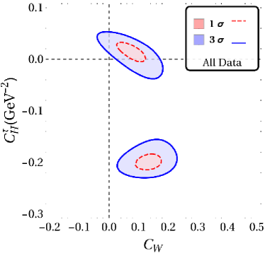
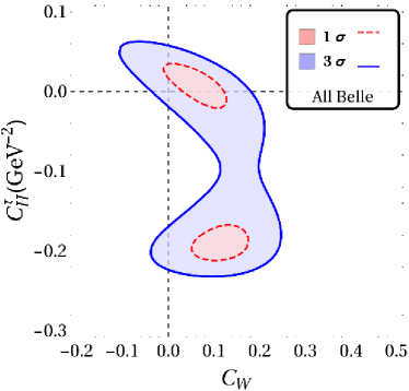
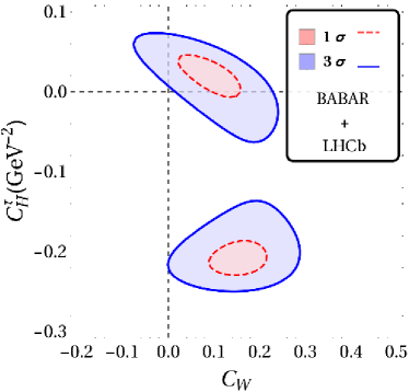
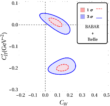
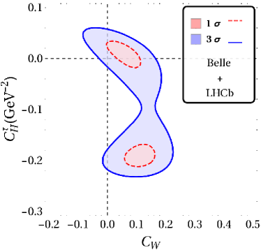
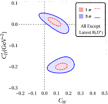
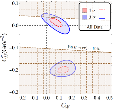
The results for our fits with a single vector and scalar type NP are displayed in fig. 2 and table. 2. In what follows $C_{S_{1}}=-C_{H}~m_{b}~m_{\ell}$ . The WC’s are considered to be real. It is clear that for all combinations of results shown in fig. 2, there is a two-fold ambiguity in the best-fit results. One of these points is closer to SM than the other and this is the one that is important in constraining NMUED. We also note that while the results from Belle and LHCb are consistent with SM within $3\sigma$ , for any and all other combination of results, the SM is away from the best fit point by more than $3\sigma$ in the $C_{W}$ - $C^{\tau}_{H}$ plane.

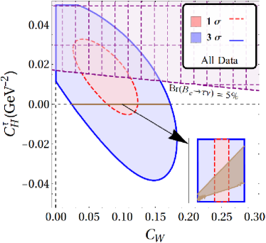
	Without $\mathcal{R}_{J/\psi}$		With $\mathcal{R}_{J/\psi}$				Fit Results		Observable values
			PQCD		LFCQ
Datasets	$\chi^{2}_{min}$	$p$ -value	$\chi^{2}_{min}$	$p$ -value	$\chi^{2}_{min}$	$p$ -value	Re( $C_{H}$ )	Im( $C_{H}$ )	$\mathcal{R}(D^{*})$	$\mathcal{R}(D)$
	/DoF	(%)	/DoF	(%)	/DoF	(%)	(GeV^-2)	(GeV^-2)
All Data	9.22/8	23.72	11.86/9	15.76	12.38/9	13.51	-0.031(8)	0.000(73)	0.2746(25)	0.448(42)
Belle	1.71/4	63.54	4.39/5	35.63	4.89/5	29.83	-0.023(11)	0.000(87)	0.2674(33)	0.406(60)
Babar +LHCb	6.42/3	4.03	9.00/4	2.92	9.54/4	2.29	-0.042(11)	0.000(84)	0.2764(34)	0.508(58)
Babar + Belle	6.71/6	24.31	9.35/7	15.48	9.87/7	13.03	-0.030(8)	0.000(74)	0.2724(25)	0.445(43)
Belle + LHCb	4.70/6	45.41	7.37/7	28.82	7.88/7	24.72	-0.025(11)	0.000(78)	0.2700(34)	0.414(59)
All $\mathcal{R}_{D^{*}}$	2.37/5	66.78	4.31/6	50.53	4.99/6	41.67	-	-
No $P_{\tau}(D^{*})$	9.21/7	16.23	11.84/8	10.58	12.36/8	8.92	-0.031(8)	0.000(72)	0.2746(25)	0.448(42)

Table 2: Results of fits for different combinations of experimental data-points along with our predictions for the charged current observables for the case with both

O_{V_{1}}

and

O_{S_{1}}

. The last two columns are obtained from fits without treating

\mathcal{R}_{J/\psi}

as a data point.

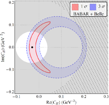
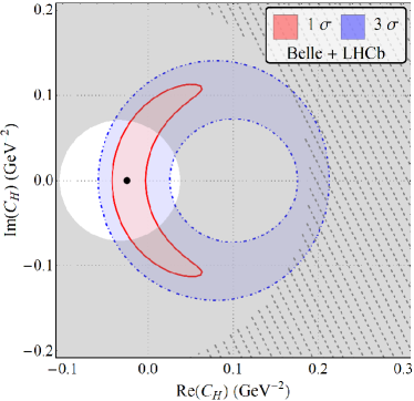
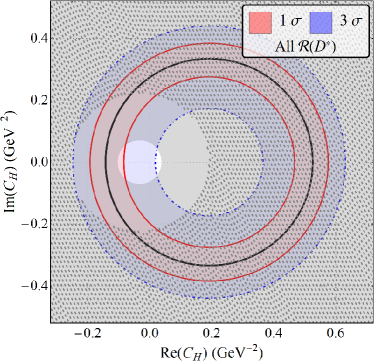
The results for our fits with a single vector and scalar type NP are displayed in fig. 3 and table. 3, assuming $c_{H}$ to be complex.

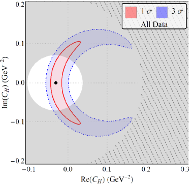
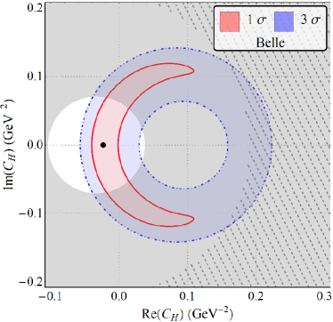
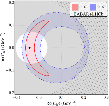
	Without $\mathcal{R}_{J/\psi}$		With $\mathcal{R}_{J/\psi}$				Fit Results
			PQCD		LFCQ
Datasets	$\chi^{2}_{min}$	$p$ -value	$\chi^{2}_{min}$	$p$ -value	$\chi^{2}_{min}$	$p$ -value	Re( $C_{H}$ )	Im( $C_{H}$ )
	/DoF	(%)	/DoF	(%)	/DoF	(%)	(GeV^-2)	(GeV^-2)
All Data	9.22/8	23.72	11.86/9	15.76	12.38/9	13.51	-0.031(8)	0.000(73)
Belle	1.71/4	63.54	4.39/5	35.63	4.89/5	29.83	-0.023(11)	0.000(87)
Babar+LHCb	6.42/3	4.03	9.00/4	2.92	9.54/4	2.29	-0.042(11)	0.000(84)
Babar+ Belle	6.71/6	24.31	9.35/7	15.48	9.87/7	13.03	-0.030(8)	0.000(74)
Belle + LHCb	4.70/6	45.41	7.37/7	28.82	7.88/7	24.72	-0.025(11)	0.000(78)
All $\mathcal{R}_{D^{*}}$	2.37/5	66.78	4.31/6	50.53	4.99/6	41.67	-	-
No $P_{\tau}(D^{*})$	9.21/7	16.23	11.84/8	10.58	12.36/8	8.92	-0.031(8)	0.000(72)

Table 3: Results of fits with different combinations of experimental data-points for the case with only

O_{S_{1}}

5 Models

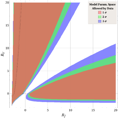
The model independent scenarios described in the previous sections are further illustrated with the help of benchmark models in this section. Details about the model parameters and their relations with $C_{S_{1}}$ and $C_{V_{1}}$ can be found in [14, 15].

5.1 Real $C_{V_{1}}$ and $C_{S_{1}}$ : Non-Minimal universal extra dimension(NMUED)

5.2 Real $C_{S_{1}}$ : Goergi Michacek model (GM)

5.3 Complex $C_{S_{1}}$ : Leptoquark model (LQ)

Data	${\rm Re}\left(g^{33}_{2L}g^{23*}_{2R}\right)$	${\rm Im}\left(g^{33}_{2L}g^{33*}_{2R}\right)$
All Data	$-0.250(64)$	$0.0(6)$
Belle	$-0.186(90)$	$0.0(7)$
Babar+LHCb	$-0.338(89)$	$0.0(7)$
Babar + Belle	$-0.245(65)$	$0.0(6)$
Belle + LHCb	$-0.198(88)$	$0.0(6)$
No $P_{\tau}\left(D^{*}\right)$	$-0.250(64)$	$0.0(6)$

Table 4: Allowed values of the product of the couplings (both real and imaginary) of the chosen Leptoquark model involved with the Wilson coefficient

C_{S_{1}}^{l}

References

[1] J. P. Lees et al. [BaBar Collaboration], Phys. Rev. Lett. 109, 101802 (2012) doi:10.1103/PhysRevLett.109.101802 [arXiv:1205.5442 [hep-ex]].
[2] J. P. Lees et al. [BaBar Collaboration], Phys. Rev. D 88, no. 7, 072012 (2013) doi:10.1103/PhysRevD.88.072012 [arXiv:1303.0571 [hep-ex]].
[3] M. Huschle et al. [Belle Collaboration], Phys. Rev. D 92, no. 7, 072014 (2015) doi:10.1103/PhysRevD.92.072014 [arXiv:1507.03233 [hep-ex]].
[4] Y. Sato et al. [Belle Collaboration], Phys. Rev. D 94, no. 7, 072007 (2016) doi:10.1103/PhysRevD.94.072007 [arXiv:1607.07923 [hep-ex]].
[5] R. Aaij et al. [LHCb Collaboration], Phys. Rev. Lett. 115, no. 11, 111803 (2015) Erratum: [Phys. Rev. Lett. 115, no. 15, 159901 (2015)] doi:10.1103/PhysRevLett.115.159901, 10.1103/PhysRevLett.115.111803 [arXiv:1506.08614 [hep-ex]].
[6] S. Hirose et al. [Belle Collaboration], Phys. Rev. Lett. 118, no. 21, 211801 (2017) doi:10.1103/PhysRevLett.118.211801 [arXiv:1612.00529 [hep-ex]].
[7] S. Hirose et al. [Belle Collaboration], Phys. Rev. D 97, no. 1, 012004 (2018) doi:10.1103/PhysRevD.97.012004 [arXiv:1709.00129 [hep-ex]].
[8] R. Aaij et al. [LHCb Collaboration], Phys. Rev. Lett. 120, no. 17, 171802 (2018) doi:10.1103/PhysRevLett.120.171802 [arXiv:1708.08856 [hep-ex]].
[9] R. Aaij et al. [LHCb Collaboration], Phys. Rev. D 97, no. 7, 072013 (2018) doi:10.1103/PhysRevD.97.072013 [arXiv:1711.02505 [hep-ex]].
[10] D. Bigi and P. Gambino, Phys. Rev. D 94, no. 9, 094008 (2016) doi:10.1103/PhysRevD.94.094008 [arXiv:1606.08030 [hep-ph]].
[11] F. U. Bernlochner, Z. Ligeti, M. Papucci and D. J. Robinson, Phys. Rev. D 95, no. 11, 115008 (2017) Erratum: [Phys. Rev. D 97, no. 5, 059902 (2018)] doi:10.1103/PhysRevD.95.115008, 10.1103/PhysRevD.97.059902 [arXiv:1703.05330 [hep-ph]].
[12] D. Bigi, P. Gambino and S. Schacht, JHEP 1711, 061 (2017) doi:10.1007/JHEP11(2017)061 [arXiv:1707.09509 [hep-ph]].
[13] S. Jaiswal, S. Nandi and S. K. Patra, JHEP 1712, 060 (2017) doi:10.1007/JHEP12(2017)060 [arXiv:1707.09977 [hep-ph]].
[14] A. Biswas, A. Shaw and S. K. Patra, Phys. Rev. D 97, no. 3, 035019 (2018) doi:10.1103/PhysRevD.97.035019 [arXiv:1708.08938 [hep-ph]].
[15] A. Biswas, D. K. Ghosh, A. Shaw and S. K. Patra, arXiv:1801.03375 [hep-ph].

b→c​l​νb\to cl\nu anomalies in light of vector and scalar interactions