BDDC by a Frontal Solver and the Stress Computation in a Hip Joint Replacement

Parallel numerical solution of linear problems arising from linearized isotropic elasticity discretized by finite elements is important in many areas of engineering. The matrix of the system is typically large, sparse, and ill-conditioned. The classical frontal solver [8] has became a popular direct method for solving problems with such matrices arising from finite element analyses. However, for large problems, the computational cost of direct solvers makes them less competitive compared to iterative methods, such as the preconditioned conjugate gradients (PCG) [4]. The goal is then to design efficient preconditioners that result in a lower overall cost and can be implemented in parallel, which has given rise to the field of domain decomposition and iterative substructuring [17].

The Balancing Domain Decomposition based on Constraints (BDDC) [6] is one of the most advanced preconditioners of this class. However, the additional custom coding effort required can be an obstacle to the use of the method in an existing finite element code. We propose an implementation of BDDC built on top of common components of existing finite element codes, namely the frontal solver and the element stiffness matrix generation. The implementation requires only a minimal amount of additional code and it is therefore of interest. For an important alternative implementation of BDDC, see [11].

BDDC is closely related to FETI-DP [7]. Though the methods are quite different, they can be built largely from the same components, and the eigenvalues of the preconditioned problem (other than the eigenvalue equal to one) in BDDC and FETI-DP are the same [13]. See also [2, 11, 14] for simplified proofs. Thus the performance of BDDC and FETI-DP is essentially identical, and results for one method apply immediately to the other.

The frontal solver was used to implement a limited variant of BDDC in [3, 16]. The implementation takes advantage of the existing integration of the frontal solver into the finite element methodology and of its implementation of constraints, which is well-suited for BDDC. However, the frontal solver treats naturally only point constraints, while an efficient BDDC method in three dimensions requires constraints on averages. This fact was first observed for FETI-DP experimentally in [7], and theoretically in [10], but these observations apply to BDDC as well because of the equivalence between the methods.

In this paper, we extend the previous implementation of BDDC by the frontal solver to constraints on averages and apply the method to a problem in biomechanics. We also compare the performance of the mehod with adding averages and with additional point constraints. The implementation relies on the separation of point constraints and enforcing the rest by Lagrange multipliers, as suggested already in [6]. One new aspect of the present approach is the use of reactions, which come naturally from the frontal solver, to avoid custom coding.

Consider the problem in a variational form

where $V$ is a finite element space of $\mathbb{R}^{3}$-valued piecewise polynomial functions $v$ continuous on a given domain $\Omega\subset\mathbb{R}^{3}$, satisfying homogeneous Dirichlet boundary conditions, and

Here $\lambda$ and $\mu$ are the first, and the second Lamé’s parameter, respectively. Solution $u\in V$ represents the vector field of displacement. It is known that $a(u,v)$ is a symmetric positive definite bilinear form on $V$. An equivalent formulation of (1) is to find a solution $u$ to a linear system

where $A=(a_{ij})$ is the stiffness matrix computed as $a_{ij}=a(\phi_{i},\phi_{j})$, where $\{\phi_{i}\}$ is a finite element basis of $V$, corresponding to set of unknowns, also called degrees of freedom, defined as values of displacement at the nodes of a given triangulation of the domain. The domain $\Omega$ is decomposed into nonoverlapping subdomains $\Omega_{i}$, $i=1,\dots N$, also called substructures. Unknowns common to at least two subdomains are called boundary unknowns and the union of all boundary unknowns is called the interface $\Gamma$.

The first step is the reduction of the problem to the interface. This is quite standard and described in the literature, e.g., [17]. The space $V$ is decomposed as the $a$-orthogonal direct sum $V=V_{1}\oplus\dots\oplus V_{N}\oplus V_{\Gamma}$, where $V_{i}$ is the space of all functions from $V$ with nonzero values only inside $\Omega_{i}$ (in particular, they are zero on $\Gamma$), and $V_{\Gamma}$ is the $a$-orthogonal complement of all spaces $V_{i}$; $V_{\Gamma}=\{v\in V:a(v,w)=0\,\,\forall w\in V_{i},\,i=1,\dots N\}$. Functions from $V_{\Gamma}$ are fully determined by their values at unknowns on $\Gamma$ and the discrete harmonic condition that they have minimal energy on every subdomain (i.e. solve the system with zero right hand side in corresponding equations). They are represented in the computation by their values on the interface $\Gamma$. Solution $u$ may be split into the sum of interior solutions $u_{o}=\sum_{i}^{N}u_{i}$, $u_{i}\in V_{i}$, and $u_{\Gamma}\in V_{\Gamma}$. Then problem (3) may be rewritten as

Let us now write problem (4) in the block form, with the first block corresponding to unknowns in subdomain interiors, and the second block corresponding to unknowns at the interface,

with $u_{o2}=0$. Using the fact that functions from $V_{\Gamma}$ are energy orthogonal to interior functions (so it holds $A_{11}u_{\Gamma 1}+A_{12}u_{\Gamma 2}=0$) and eliminating the variable $u_{o1}$, we obtain that (5) is equivalent to

and the solution is obtained as $u=u_{\Gamma}+u_{o}$. Problem (7) is equivalent to the problem

where $S$ is the Schur complement with respect to interface: $S=A_{22}-A_{21}A_{11}^{-1}A_{12}$, and $g_{2}$ is the condensed right hand side $g_{2}=f_{2}-A_{21}u_{o1}=f_{2}-A_{21}A_{11}^{-1}f_{1}$. Problem (8) can be split into two problems

Since $A_{11}$ has a block diagonal structure, the solution to (6) may be found in parallel and similarly the solution to (9).

The BDDC method is a particular kind of preconditioner for the reduced problem (10). The main idea of the BDDC preconditioner in an abstract form [14] is to construct an auxiliary finite dimensional space $\widetilde{W}$ such that $V_{\Gamma}\subset\widetilde{W}$ and extend the bilinear form $a\left(\cdot,\cdot\right)$ to a form $\widetilde{a}\left(\cdot,\cdot\right)$ defined on $\widetilde{W}\times\widetilde{W}$ and such that solving the variational problem (1) with $\widetilde{a}\left(\cdot,\cdot\right)$ in place of $a\left(\cdot,\cdot\right)$ is cheaper and can be split into independent computations done in parallel. Then the solution projected to $V_{\Gamma}$ is used for the preconditioning of $S$. Specifically, let $E:\widetilde{W}\rightarrow V_{\Gamma}$ be a given projection of $\widetilde{W}$ onto $V_{\Gamma}$, and $r_{2}={g}_{2}-Su_{\Gamma 2}$ the residual in a PCG iteration. Then the output of the BDDC preconditioner is the part $v_{2}$ of $v=Ew$, where

In terms of operators, $v=E\widetilde{S}^{-1}E^{T}r$, where $\widetilde{S}$ is the operator on $V_{\Gamma}$ associated with the bilinear form $\widetilde{a}$ (but not computed explicitly as a matrix).

Note that while the residual $r_{2}$ in the PCG method applied to the reduced problem is given at the interface only, the residual in (11) has the dimension of all unknowns on the subdomain. This is corrected naturally by extending the residual $r_{2}$ to subdomain interiors by zeros (setting $r_{1}=0$), which is required by the condition that the solution $v$ is discrete harmonic inside subdomain. Similarly, only interface values $v_{2}$ of $v$ are used in further PCG computation. Such approach is equivalent to computing with explicit Schur complements.

The choice of the space $\widetilde{W}$ and the projection $E$ determines a particular instance of BDDC [6, 14]. All functions from $V_{\Gamma}$ are continuous on the domain $\Omega$. In order to design the space $\widetilde{W}$, we relax the continuity on the interface $\Gamma$. On $\Gamma$, we select coarse degrees of freedom and define $\widetilde{W}$ as the space of finite element functions with minimal energy on every subdomain, continuous across $\Gamma$ only at coarse degrees of freedom. The coarse degrees of freedom can be of two basic types – explicit unknowns (called coarse unknowns) at selected nodes (called corners), and averages over larger sets of nodes (subdomain faces or edges). The continuity condition then means that the values at the corresponding corners, resp. averages, on neighbouring subdomains coincide. The bilinear form $a\left(\cdot,\cdot\right)$ from (2) is extended to $\widetilde{a}\left(\cdot,\cdot\right)$ on $\widetilde{W}\times\widetilde{W}$ by integrating (2) over the subdomains $\Omega_{i}$ separately and adding the results.

The projection $E:\widetilde{W}\rightarrow V_{\Gamma}$ is defined at unknowns on the interface $\Gamma$ (the $u_{\Gamma 2}$ part) as a weighted average of values from different subdomains and thus resulting in function continuous across the interface. These averaged values on $\Gamma$ determine the projection $E$, because values inside subdomains (the $u_{\Gamma 1}$ part) are then obtained by the solutions of local subdomain problems (9) to make the averaged function discrete harmonic. To assure good performance regardless of different stiffness of the subdomains [12], the weights are chosen proportional to the corresponding diagonal entries of the subdomain stiffness matrices. The transposed projection $E^{T}$ is used for distribution of the residual $r_{2}$ among neighbouring subdomains and represents the decomposition of unity at unknowns on interface.

The decomposition into subspaces used to derive the problem with Schur complement (10) is now repeated for space $\widetilde{W}$, with the coarse degrees of freedom playing the role of interface unknowns and $\widetilde{a}(\cdot,\cdot)$ the role of $a(\cdot,\cdot)$. Namely, space $\widetilde{W}$ is decomposed as $\widetilde{a}$-orthogonal direct sum $\widetilde{W}=\widetilde{W}_{1}\oplus\dots\oplus\widetilde{W}_{N}\oplus\widetilde{W}_{C}$, where $\widetilde{W}_{i}$ is the space of functions with nonzero values only in $\Omega_{i}$ outside coarse degrees of freedom (they have zero values at corners, they are generally not continuous at other unknowns on $\Gamma$, and they have zero averages) and $\widetilde{W}_{C}$ is the coarse space, defined as the $\widetilde{a}$-orthogonal complement of all spaces $\widetilde{W}_{i}$: $\widetilde{W}_{C}=\{v\in\widetilde{W}:\widetilde{a}(v,w)=0\ \forall w\in\widetilde{W}_{i},\ i=1,\dots N\}$. Functions from $\widetilde{W}_{C}$ are fully determined by their values at coarse degrees of freedom (where they are continuous) and have minimal energy. Thus, they are generally discontinuous across $\Gamma$ outside the corners. The solution $w\in\widetilde{W}$ from (11) is now split accordingly as $w=w_{C}+\sum_{i=1}^{N}w_{i},$ where $w_{C}$, determined by

is called the coarse correction, and $w_{i}$, determined by

is the substructure correction from $\Omega_{i}$, $i=1,\dots N$.

Let us now rewrite the BDDC preconditioner in terms of matrices, following [6]. Problem (13) is formulated in a saddle point form as

where $K_{i}$ denotes the substructure local stiffness matrix, obtained by the subassembly of element matrices only of elements in substructure $i$, matrix $\overline{C}_{i}$ represents constraints on subdomain, that enforce zero values of coarse degrees of freedom, $\mu_{i}$ is vector of Lagrange multipliers, and $r_{i}$ is the weighted residual $E^{T}r$ restricted to subdomain $i$.

Matrix $K_{i}$ is singular for floating subdomains (subdomains not touching Dirichlet boundary conditions), while the augmented matrix of problem (14) is regular and may be factorized. Matrix $\overline{C}_{i}$ contains both constraints enforcing continuity across corners (single point continuity), and constraints enforcing equality of averages over edges and faces of subdomains. The former type corresponds to just one nonzero entry equal to 1 on a row of $\overline{C}_{i}$, while the latter leads to several nonzero entries on a row. This structure will be exploited in the following section.

Problem (14) is solved in each iteration of the PCG method to find the correction from substructure $i$. However, the matrix of (14) is used prior the whole iteration process to construct the local subdomain matrix of the coarse problem. First, the coarse basis functions are found independently for each subdomain as the solution to

This is a problem with multiple right hand sides, where $\psi_{i}$ is a matrix of coarse basis functions with several columns, each corresponding to one coarse degree of freedom on subdomain. These functions are given by values equal to 0 at all coarse degrees of freedom except one, where they have value equal to 1, and they have minimal energy on subdomain outside coarse degrees of freedom. The identity block $I$ has the dimension of the number of constraints on the subdomain.

Once $\psi_{i}$ is known, the subdomain coarse matrix $K_{Ci}$ is constructed as

Matrices $K_{Ci}$ are then assembled to form the global coarse matrix $A_{C}$. This procedure is same as the standard process of assembly in finite element solution, with subdomains playing the role of elements, coarse degrees of freedom on subdomain representing degrees of freedom on element, and matrix $K_{Ci}$ representing the element stiffness matrix.

Problem (12) is now

where $r_{C}$ is the global coarse residual obtained by the assembly of the subdomain contributions of the form $r_{Ci}=\psi_{i}^{T}r_{i}$.

The coarse solution $\mathbf{w}_{C}$ has the dimension of the number of all coarse degrees of freedom. So, to add the correction to subdomain problems, we first have to restrict it to coarse degrees of freedom on each subdomain and to interpolate it to the whole subdomain by $w_{Ci}=\psi_{i}\mathbf{w}_{Ci}$. By extending $w_{Ci}$ and $w_{i}$ by zero to other subdomains, these can be summed over the subdomains to form the final vector $w$. Finally, the preconditioned residual is obtained as $v=Ew$.

It is worth noticing that in the case of no constraints on averages, i.e. using only coarse unknowns for the definition of the coarse space, matrix $A_{C}$ of problem (17) is simply the Schur complement of matrix $A$ with respect to coarse unknowns. This fact was pointed out in [11]. If additional degrees of freedom are added for averages, they correspond to new explicit unknowns in $\mathbf{w}_{Ci}$.

Obviously, several mapping operators among various spaces are needed in the implementation, defining embedding of subdomains into global problem, local subdomain coarse problem into global coarse problem etc. We have circumvented their mathematical definition by words for the sake of brevity, while we refer to [6, 12] for rigorous definitions of these operators.

The frontal solver implements the solution of a square linear system with some of the variables having prescribed values. Equations that correspond to the fixed variables are omitted and the values of these variables are substituted into the solution vector directly. The output of the solver consists of the solution and the resulting imbalance in the equations, called reaction forces. More precisely, consider a block decomposition of the vector of unknowns $x$ with the second block consisting of all fixed variables, and write a system matrix $A$ with the same block decomposition (here, the decomposition is different from the one in Section 2). Then on exit from the frontal solver,

where fixed variable values $x_{2}$ and the load vectors $f_{1}$ and $f_{2}$ are the inputs, while the solution $x_{1}$ and the reaction $r_{2}$ are the outputs. Stiffness matrices of elements are input instead of the whole matrix, and their assembly is done simultaneously with the factorization inside the frontal solver.

The key idea of this section is to split the constraints in matrix $\overline{C}_{i}$ and to handle them in different ways. Those enforcing zero values at corners will be enforced as fixed variables, while the remaining constraints, corresponding to averages and denoted $C_{i}$, will be still enforced using Lagrange multipliers.the

In the rest of this section, we drop the subdomain subscript _i and we write subdomain vectors $w$ in the block form with the second block consisting of unknowns that are involved in coarse degrees of freedom (i.e. coarse unknowns), denoted by the subscript _c, and the first block consisting of the remaining degrees of freedom, denoted by the subscript _f. The vector of the coarse degrees of freedom given by averages is written as $Cw$, where each row of $C$ contains the coefficients of the average that makes that degree of freedom. Then subdomain vectors $w\in\widetilde{W}$ are characterized by $w_{c}=0$, $Cw=0$. Assume that $C=\left[C_{f}\ \ C_{c}\right]$, with $C_{c}=0$, that is, the averages do not involve single variable coarse degrees of freedom; then $Cw=C_{f}w_{f}$. The subdomain stiffness matrix $K$ is singular for floating subdomains, but the block $K_{ff}$ is nonsingular if there are enough corners to eliminate the rigid body motions, which will be assumed.

We now show how to solve (14) – (17) using the frontal solver. In the case when there are no averages as coarse degrees of freedom, we recover the previous method from [3, 16].

The local substructure problems (13) are written in the frontal solver form (18) as

where $w_{c}=0$, $r$ is the part in the _f block of the residual in the PCG method distributed to the substructures by the operator $E^{T}$, and $Rea$ is the reaction. The constraint $w_{c}=0$ is enforced by marking the $w_{c}$ unknowns as fixed, while the remaining constraints $C_{f}w_{f}=0$ are enforced via the Lagrange multiplier $\mu$. Using the fact that $w_{c}=0$, we get from (19) that

From (20), $w_{f}=K_{ff}^{-1}\left(-C_{f}^{T}\mu+r\right)$. Now substituting $w_{f}$ into (22), we get the problem for Lagrange multiplier $\mu$,

The matrix $C_{f}K_{ff}^{-1}C_{f}^{T}$ is dense but small, with the order equal to the number of averages on the subdomain, and it is constructed by solving the system $K_{ff}U=C_{f}^{T}$ with multiple right hand sides by the frontal solver and then the multiplication $C_{f}U$. After solving problem (23), we substitute for $\mu$ in (20) and find $w_{f}$ from

by the frontal solver, considering $w_{c}=0$ fixed. The factorization in the frontal solver for (24) and the factorization of the matrix $C_{f}K_{ff}^{-1}C_{f}^{T}$ for (23) need to be computed only once in the setup phase.

The coarse problem (17) is solved by the frontal solver just like a finite element problem, with the subdomains playing the role of elements. It only remains to specify the basis functions of $\widetilde{W}_{C}$ on the subdomain from (15), and compute the local subdomain coarse matrix (16) efficiently. Denote by $\psi^{c}$ the matrix whose colums are coarse basis functions associated with the coarse unknowns at corners, and $\psi^{avg}$ the matrix made out of the coarse basis functions associated with averages. To find the coarse basis functions, we proceed similarly as in (19) and write the equations for the coarse basis functions in the frontal solver form, now with multiple right-hand sides,

where $Rea^{c}$ and $Rea^{avg}$ are matrices of reactions. Denote $\psi_{f}=\left[\begin{array}[c]{cc}\psi_{f}^{c}&\psi_{f}^{avg}\end{array}\right]$, $\psi_{c}=\left[\begin{array}[c]{cc}\psi_{c}^{c}&\psi_{c}^{avg}\end{array}\right]=\left[\begin{array}[c]{cc}I&0\end{array}\right]$, $\lambda=\left[\begin{array}[c]{cc}\lambda^{c}&\lambda^{avg}\end{array}\right]$, $Rea=\left[\begin{array}[c]{cc}Rea^{c}&Rea^{avg}\end{array}\right]$, and $R=\left[\begin{array}[c]{cc}0&I\end{array}\right]$. Then (25) becomes

From (26), we get $\psi_{f}=-K_{ff}^{-1}\left(K_{fc}\psi_{c}+C_{f}^{T}\lambda\right)$. Substituting $\psi_{f}$ into (28), we derive the problem for Lagrange multipliers

which is solved for $\lambda$ by solving the system (29) for multiple right hand sides. Since $\psi_{c}$ is known, we can use the frontal solver to solve (26)-(27) to find $\psi_{f}$ and $Rea$:

considering $\psi_{c}$ fixed. Finally, we construct the local coarse matrix corresponding to the subdomain as

where $\psi=\left[\begin{array}[c]{cc}\psi^{c}&\psi^{avg}\end{array}\right]$.

At the end of the setup phase, the matrix of coarse problem is factored by the frontal solver, using subdomain coarse matrices as input.

The setup starts with two types of factorization of the system matrix by frontal algorithm that differ only in the set of fixed variables. In the first factorization, all interface unknowns are prescribed as fixed, for the solution of problems (5) and (7). In the second factorization, only the coarse unknowns are fixed, for the solution of problems (24) and (30). Both factorizations are done subdomain by subdomain, so the interface unknowns are represented by their own instance in different subdomains. This naturally leads to parallelization according to subdomains. Then the main steps of the algorithm are as follows.

(A) Solve (6) in parallel on every subdomain for $g_{2}$ as reaction using the frontal solver with $u_{o2}=0$ fixed,

(B) Solve (10) for $u_{\Gamma 2}$ using PCG with BDDC preconditioner (for more details see bellow).
(C) Compute the solution $u$ from (5) using the frontal solver with $u_{\Gamma 2}$ fixed and $u_{o2}=0$.

Step (B) in detail follows. Before starting cycle of PCG iterations, compute in advance:

• •

  Matrix $C_{f}K_{ff}^{-1}C_{f}^{T}$ of (23), resp. (29) and its factorization.

• •

  Coarse basis functions $\psi_{i}$ of (15) from (30). Multiplier $\lambda$ on the right hand side of (30) is computed from (29).

• •

  Local matrices $K_{Ci}$ of (16) from (31).

• •

  Factorization of matrix $A_{C}$ of (17) using the frontal solver with local coarse matrices $K_{Ci}$ as ‘element’ matrices.

• •

  The first residual $r_{2}$ of (10) from the first approximation of $u_{\Gamma 2}$ using the frontal solver on (7) with $u_{\Gamma 2}$ fixed,

  $$\left[\begin{array}[c]{cc}A_{11}&A_{12}\\ A_{21}&A_{22}\end{array}\right]\left[\begin{array}[c]{c}u_{\Gamma 1}\\ u_{\Gamma 2}\end{array}\right]=\left[\begin{array}[c]{c}0\\ g_{2}\end{array}\right]+\left[\begin{array}[c]{c}0\\ -r_{2}\end{array}\right].$$

  (33)

  For the popular choice of initial solution $u_{\Gamma 2}=0$, this step reduces to setting $r_{2}=g_{2}$ (the discrete harmonic extension of zero function on interface is zero also in the interior of subdomain).

Then in every PCG iteration, compute $v_{2}$ from $r_{2}$ in three steps:

1. 1.

   Compute $E^{T}r$ by distributing the residual $r_{2}$ on interface $\Gamma$ among neigbouring subdomains.
   For every subdomain, compute $r_{i}$ as restriction of $E^{T}r$ to that subdomain.

2. 2.

   Compute $w=\widetilde{S}^{-1}E^{T}r$ as sum of all substructure corrections $w_{i}$ and coarse correction $w_{C}$. These can be computed in parallel for every $r_{i}$:

   • •

     Substructure correction $w_{i}$ given by (14) is computed from (24) using frontal with $w_{c}=0$ fixed. Multiplier $\mu$ on the right hand side of (24 ) is computed from (23) and $r$ in both (24) and (23) is the part in the _f block of the $r_{i}$.

   • •

     Coarse correction $w_{C}$ is solution of (17).

   We are interested in values of $w$ only on interface.

3. 3.

   Compute the $v_{2}$ part of $v=Ew$ at every interface node as weighted average of values of $w$ at that node (neigbouring subdomains have generally different values of $w$ at corresponding interface nodes).

Note that in every iteration of PCG, the product $Sp_{2}$ is needed, where $p_{2}$ is a search direction. This product is computed using the frontal solver with $p_{2}$ fixed,

The interior part $p_{1}$ is computed only as a by-product, and it is not used in the PCG iterations.

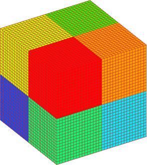
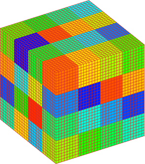
The implementation was first tested on the problem of unit cube, a classical test problem of domain decomposition methods. In our case, the cube is made of steel with Young’s modulus $2.1\cdot 10^{11}$ Pa and Poisson’s ratio $0.3$. The cube is fixed at one face and loaded by the force of $1,000$ N, acting on one edge opposite to the fixed face in direction parallel to it and pointing outwards of the cube. The mesh consists of $32^{3}=32,768$ trilinear elements. It was uniformly divided into $8$ and $64$ subdomains, resulting in $H/h=16$ and $H/h=8$, respectively (here $H$ denotes the characteristic size of subdomains and $h$ the characteristic size of elements). These divisions are presented in Figure 1. The interface is initially divided into $7$ corners, $6$ edges, and $12$ faces in the case of $8$ subdomains, and into $81$ corners, $108$ edges, and $144$ faces in the case of $64$ subdomains.

All experiments with this problem were computed on 8 1.5 GHz Intel Itanium 2 processors of SGI Altix 4700 computer in CTU Supercomputing Centre, Prague. The stopping criterion of PCG was chosen as $\|r\|_{2}/\|g\|_{2}<10^{-6}$. In the presented results, an external parallel multifrontal solver MUMPS [1] was used for the factorization and solution of the coarse problem (17), instead of the serial frontal solver.

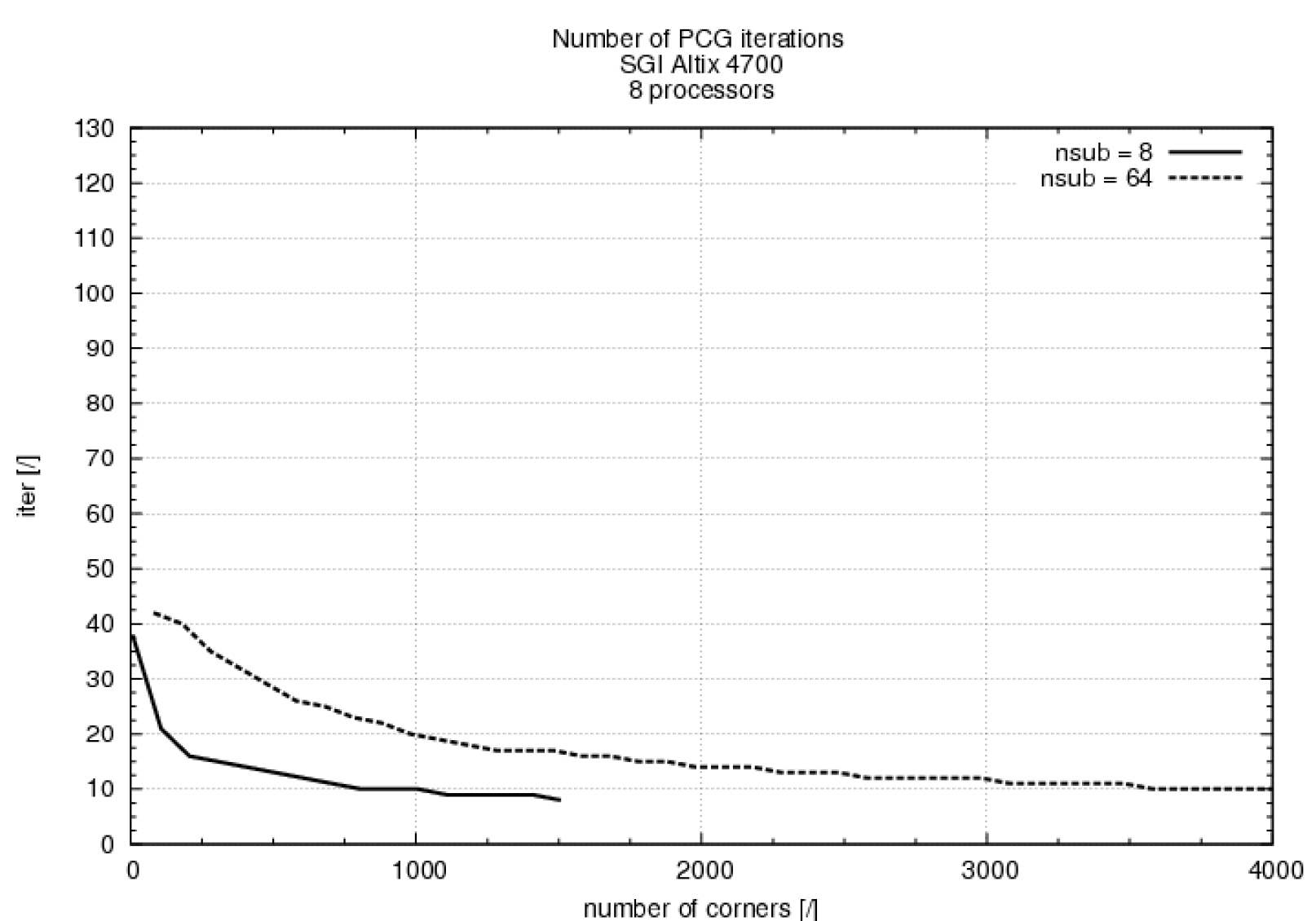
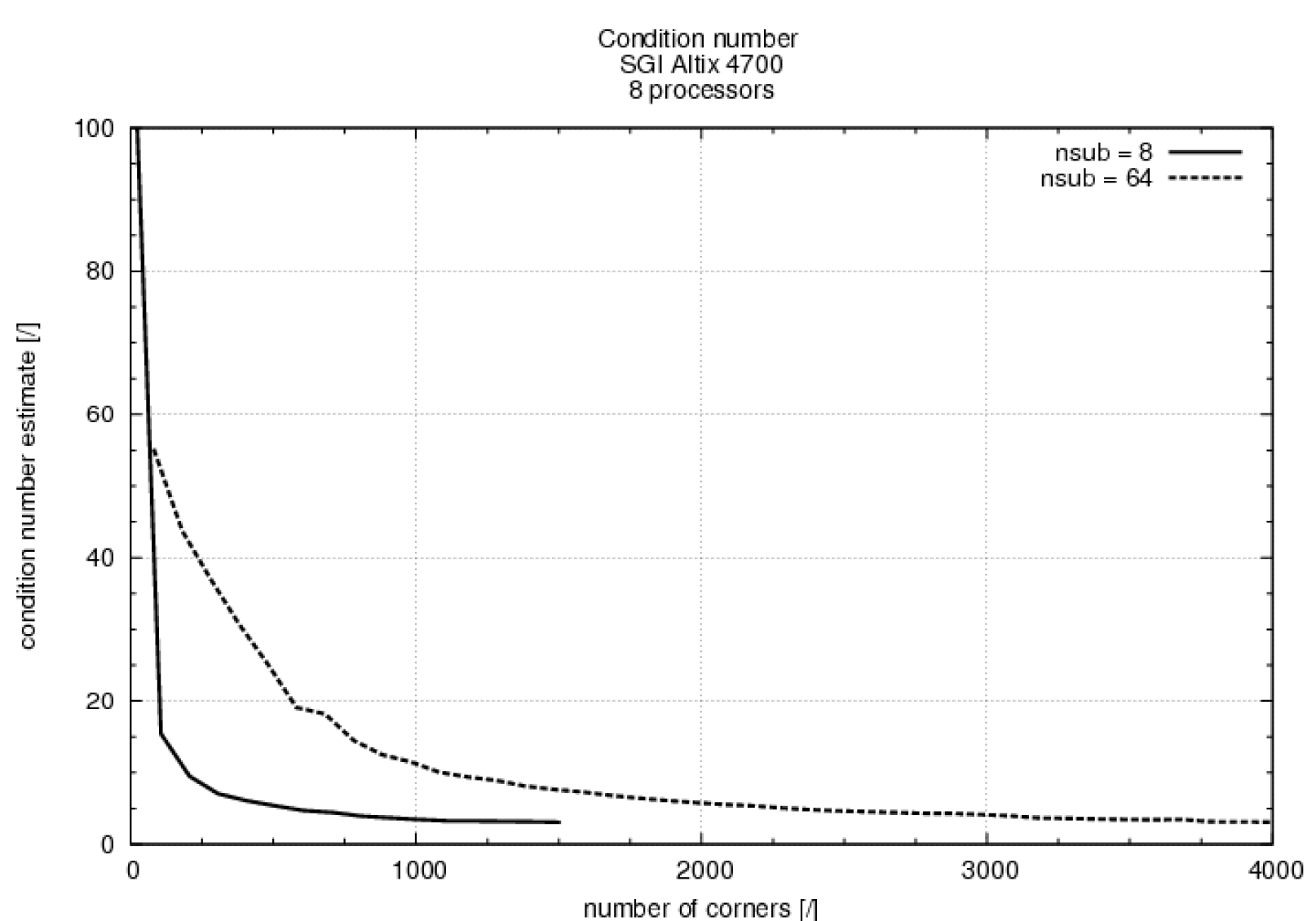
The first experiment compares two ways of enriching the coarse space $\widetilde{W}_{C}$, namely by adding point constraints on randomly selected variables on the substructure interfaces, i.e. adding more “corners” (Fig. 2 – 4), and by adding averages to the initial set of corners (Table 1 and Table 2). In the first column of these tables, no additional averages are considered and only corners were used in the construction of $\widetilde{W}_{C}$. Then we enforce the equality of arithmetic averages over all edges, over all faces, and over all edges and faces, respectively.

Although adding corners leads to an improvement of preconditioner in terms of the condition number (Fig. 3) and the number of iterations (Fig. 2), after a slight decrease early on the total computational time increases (Fig. 4) due to the added cost of the setup and factorization of the coarse problem. This effect is particularly pronounced with $8$ subdomains, where the cost of creating the coarse matrix dominates, as the frontal solver internally involves multiplication of large dense matrices to compute reactions: (30) takes $O(n_{i}n_{ci}^{2})$ for multiple right hand sides, where $n_{i}$ is the number of variables and $n_{ci}$ is the number of coarse variables in subdomain $i$. The problem divided into $64$ subdomains requires much less time than the problem with $8$ subdomains also due to the fact that the factorization time for subdomain problems grows fast with subdomain size. Note that for $64$ subdomains, the number of processors remains the same and each of the $8$ processors handles $8$ subdomains.

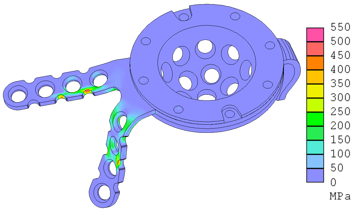
The structural analysis of the replacement of the hip joint construction loaded by pressure from body weight is an important problem in bioengineering. The hip replacement consists of several parts made of titanium; here we consider the central part of the replacement joint. The problem was simplified to stationary linearized elasticity. The highest stress was reached in the notches of the holders. In the original design, holders of the hip replacement had thickness of $2$ mm, which led to maximal von Mises stress about $1,500$ MPa. As the yield point of titanium is about $800$ MPa, the geometry of the construction had to be modified. The thickness of the holders was increased to 3 mm, radiuses of the notches were increased, and the notches were made smaller, as in Fig. 5. The maximal von Mises stress on this new construction was only about 540 MPa, which satisfed the demands for the strength of the construction [5, 18]. The mesh consists of 33,186 quadratic elements resulting in 544,734 unknowns.

The computation needs 400 minutes when using a serial frontal solver on Compaq Alpha server ES47 at the Institute of Thermomechanics, Academy of Sciences of the Czech Republic. With 32 subdomains and corner coarse degrees of freedom only, BDDC on a single Alpha processor took 10 times less, only 40 minutes.

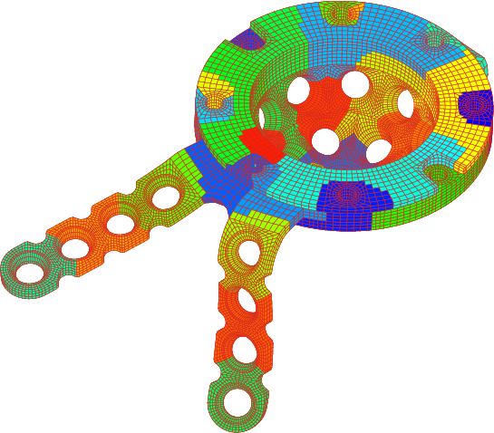
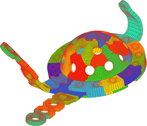
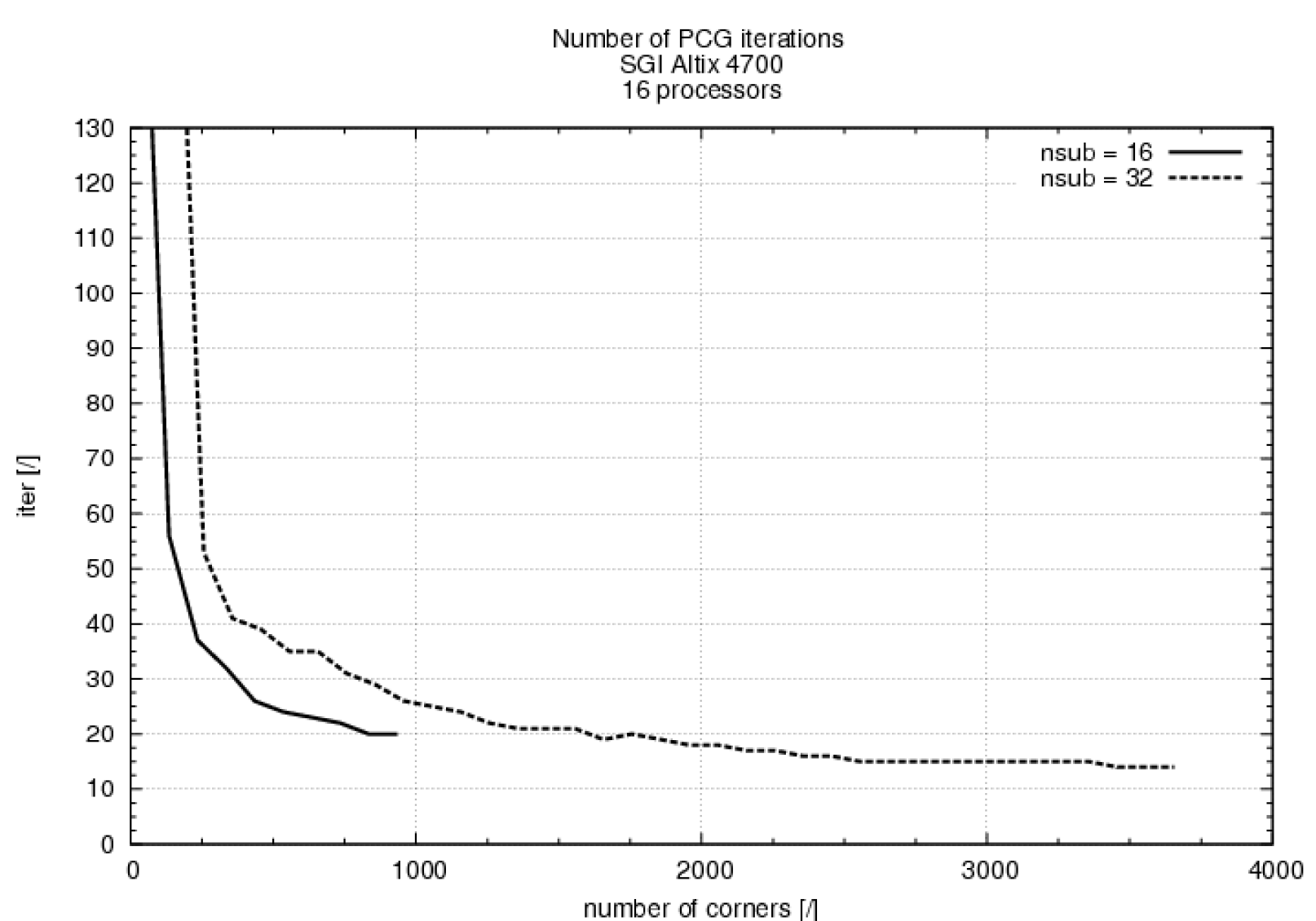
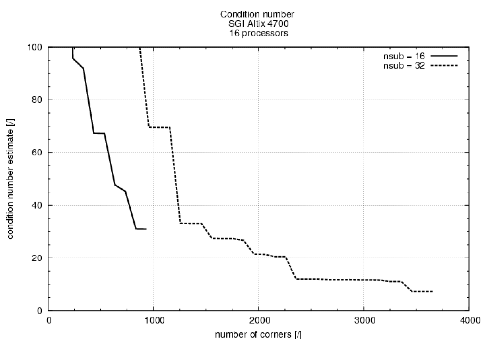
In this paper, we present results for decompositions into 16 and 32 subdomains obtained by the METIS graph partitioner [9]. In the case of 16 subdomains, the interface topology leads to 35 corners, 12 edges, and 35 faces, and in the case of 32 subdomains, to 57 corners, 12 edges, and 66 faces. All presented results were obtained on 16 processors of SGI Altix 4700. Again, the stopping criterion of PCG was chosen as $\|r\|_{2}/\|g\|_{2}<10^{-6}$. Also these results were obtained using MUMPS solver for the coarse problem solution.

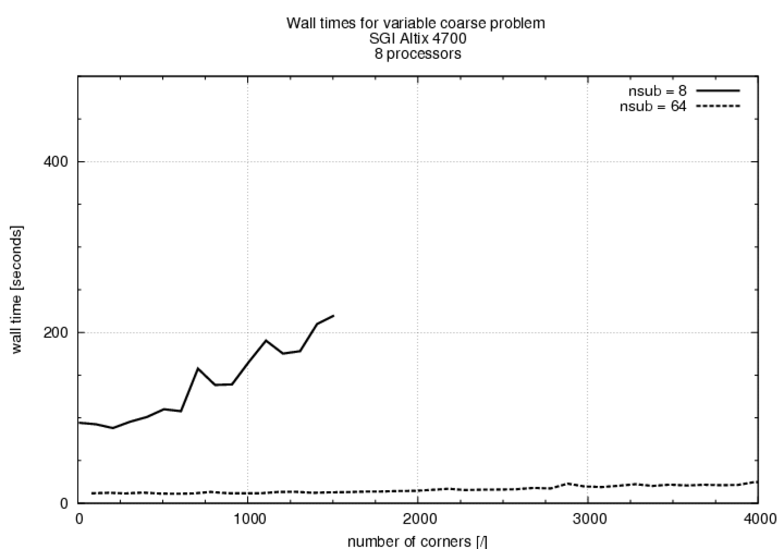
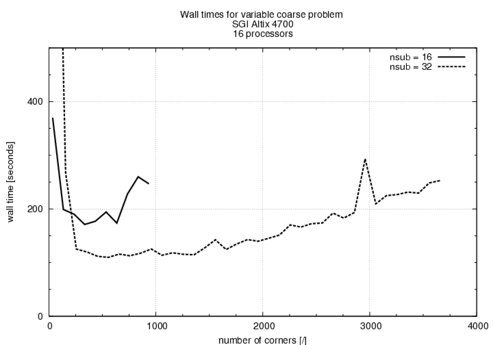
We again investigate the two approaches to coarse space enrichment. The results of random addition of corners are presented in Figures 7 – 9. Unlike in the case of the cube, a substantial decrease of the total time is achieved. The optimal number of additional corners depends on the division into subdomains.

Results of adding averages are summarized in Table 3 for the case of 16 subdomains, and in Table 4 for the case of 32 subdomains, both with the initial set of corners.

The last experiment combines both approaches: we add averages to the optimal size of the set of corners, determined from Figure 9 as ${\sim}335$ for the problem with $16$ subdomains, and ${\sim}557$ for the problem with $32$ subdomains. These results are presented in Tables 5 and 6. We can see that this synergy can lead to the lowest overall time of the computation.

We observe that while the implementation of averages leads to a negligible increase in the computational cost of the factorizations, it considerably improves the condition number, and thus reduces the overall time of solution. Also, the decomposition into 32 subdomains leads to significantly lower computational times than the division into 16 subdomains. Note that although the initial set of corners leads to non-singular local matrices and the coarse matrix and so successful setup of the preconditioner, the iterations do not converge in this case.

We have presented an application of a standard frontal solver within the iterative substructuring method BDDC. The method was applied to a biomechanical stress analysis problem. The numerical results show that the improvement of preconditioning by additional constraints is significant and can lead to a considerable savings of computational time, while the additional cost is negligible.

For a model problem (cube), constraints by averages on edges and faces are required for good performance, as predicted by the theory [10, 13], and additional point constraints (i.e., corners) are not productive. However, for the hip replacement problem (which is far from a regularly decomposed cube), additional point constraints result in significantly lower total computational time than the averages, and the best result is obtained by combining both the added point constraints and the averages.

For large problems and a large number of processors, load balancing will be essential [15].

This research has been supported by the Czech Science Foundation under grant 106/08/0403 and by the U.S. National Science Foundation under grant DMS-0713876. It has also been partly supported by the Czech Republic under projects MSM6840770001 and AV0Z20760514. A part of this work was done while Jakub Šístek was visiting at the University of Colorado Denver. Another part of the work was performed during the stay of Jakub Šístek and Marta Čertíková at Edinburgh Parallel Computing Center funded by HPC-Europa project (RII3-CT-2003-506079). The authors would also like to thank Bedřich Sousedík for his help in both typesetting and proofreading of the manuscript.

References

- [1] P. R. Amestoy, I. S. Duff, J.-Y. L’Excellent, Multifrontal parallel distributed symmetric and unsymmetric solvers, Comput. Methods Appl. Mech. Engrg. 184 (2000) 501–520.
- [2] S. C. Brenner, L.-Y. Sung, BDDC and FETI-DP without matrices or vectors, Comput. Methods Appl. Mech. Engrg. 196 (8) (2007) 1429–1435.
-
[3]
P. Burda, M. Čertíková, J. Novotný, J. Šístek, BDDC
method with simplified coarse problem and its parallel implementation, in:
Proceedings of MIS 2007, Josefuv Dul, Czech Republic, January 13–20,
Matfyzpress, Praha, 2007, pp. 3–9.
URL http://ulita.ms.mff.cuni.cz/pub/MIS/MIS2007.pdf - [4] P. Concus, G. H. Golub, D. P. O’Leary, A generalized conjugate gradient method for the numerical solution of elliptic PDE, in: J. R. Bunch, D. J. Rose (eds.), Sparse Matrix Computations, Academic Press, New York, 1976, pp. 309–332.
- [5] M. Čertíková, J. Tuzar, B. Sousedík, J. Novotný, Stress computation of the hip joint replacement using the finite element method, in: Proceedings of Software a algoritmy numerické matematiky, Srní, Czech Republic, September, Charles University, Praha, 2005, pp. 31–40.
- [6] C. R. Dohrmann, A preconditioner for substructuring based on constrained energy minimization, SIAM J. Sci. Comput. 25 (1) (2003) 246–258.
- [7] C. Farhat, M. Lesoinne, K. Pierson, A scalable dual-primal domain decomposition method, Numer. Linear Algebra Appl. 7 (2000) 687–714, Preconditioning techniques for large sparse matrix problems in industrial applications (Minneapolis, MN, 1999).
- [8] B. M. Irons, A frontal solution scheme for finite element analysis, Internat. J. Numer. Methods Engrg. 2 (1970) 5–32.
- [9] G. Karypis, V. Kumar, A fast and high quality multilevel scheme for partitioning irregular graphs, SIAM J. Sci. Comput. 20 (1) (1998) 359–392 (electronic).
- [10] A. Klawonn, O. B. Widlund, M. Dryja, Dual-primal FETI methods for three-dimensional elliptic problems with heterogeneous coefficients, SIAM J. Numer. Anal. 40 (1) (2002) 159–179.
- [11] J. Li, O. B. Widlund, FETI-DP, BDDC, and block Cholesky methods, Internat. J. Numer. Methods Engrg. 66 (2) (2006) 250–271.
- [12] J. Mandel, C. R. Dohrmann, Convergence of a balancing domain decomposition by constraints and energy minimization, Numer. Linear Algebra Appl. 10 (7) (2003) 639–659.
- [13] J. Mandel, C. R. Dohrmann, R. Tezaur, An algebraic theory for primal and dual substructuring methods by constraints, Appl. Numer. Math. 54 (2) (2005) 167–193.
- [14] J. Mandel, B. Sousedík, BDDC and FETI-DP under minimalist assumptions, Computing 81 (2007) 269–280.
- [15] O. Medek, J. Kruis, Z. Bittnar, P. Tvrdík, Static load balancing applied to schur complement method, Comput. Struct. 85 (9) (2007) 489–498.
- [16] J. Šístek, M. Čertíková, P. Burda, E. Neumanová, S. Pták, J. Novotný, A. Damašek, Development of an efficient parallel BDDC solver for linear elasticity problems, in: Blaheta, R. and Starý, J. (ed.), Proceedings of Seminar on Numerical Analysis, SNA’07, Ostrava, Czech Republic, January 22–26, Institute of Geonics AS CR, Ostrava, 2007, pp. 105–108.
- [17] A. Toselli, O. Widlund, Domain decomposition methods—algorithms and theory, vol. 34 of Springer Series in Computational Mathematics, Springer-Verlag, Berlin, 2005.
- [18] J. Tuzar, Mathematical modeling of hip joint replacement. (matematické modelování náhrady kyčelního kloubu, in czech), master thesis (2005).