Beamforming Design for Joint Target Sensing and Proactive Eavesdropping††thanks: Manuscript received.
Abstract
This work studies the beamforming design in the joint target sensing and proactive eavesdropping (JTSAPE) system. The JTSAPE base station (BS) receives the information transmitted by the illegal transmitter and transmits the waveform for target sensing. The shared waveform also serves as artificial noise to interfere with the illegal receiver, thereby achieving proactive eavesdropping. We firstly optimize the transmitting beam of the BS to maximize the eavesdropping signal-to-interference-plus-noise ratio or minimize the target estimation parameter Cramér-Rao bound, respectively. Then, the joint optimization of proactive eavesdropping and target sensing is investigated, and the normalized weighted optimization problem is formulated. To address the complexity of the original problem, the formulated problem is decomposed into two subproblems: proactive eavesdropping and target sensing, which are solved by the semi-definite relaxation technique. Furthermore, the scenario in which the quality of the eavesdropping channel is stronger than that of the illegal channel is considered. We utilize the sequential rank-one constraint relaxation method and iteration technique to obtain the high-quality suboptimal solution of the beam transmit covariance matrix. Numerical simulation shows the effectiveness of our proposed algorithm.
Index Terms:
Joint target sensing and proactive eavesdropping (JTSAPE), beamforming design, eavesdropping signal-to-noise ratio (SNR), Cramér-Rao bound (CRB).I Introduction
I-A Background and Related Works
Integrated sensing and communication (ISAC) technology can share spectrum, hardware platforms, and even baseband waveforms and signal processing between communication and sensing to improve the spectral efficiency, energy efficiency, and hardware efficiency of the system for integration gain. Further, the mutual assistance and mutual gain of the two functions can also be used to improve each other’s performance and obtain coordination gain [1]-[4].
Recently, the performance for various ISAC systems was investigated to achieve concurrent sensing and communication, which were classified into the radar-centric systems [5]-[9], the communication-centric systems [10]-[13], and the joint-design systems [14]-[15]. The authors in [5] investigated beamforming designs for the ISAC systems with multiple communication users (CUs) for scenarios with point or extended targets. In particular, the Cramér-Rao bound (CRB) of the azimuth angle or the response matrix of the target was minimized by designing the dual-functional beamforming matrix. The authors in [6] proposed an integrated sensing, communication, and computation over-the-air framework to enable simultaneous communication, target sensing, and over-the-air computation (AirComp). The shared and separated schemes were proposed, and the accuracy of AirComp was optimized by jointly designing the data transmission beamformer and the aggregation beamformer or the data beamformer and the radar sensing beamformer. In [7], a new angular waveform similarity metric was proposed and combined with the integrated main-lobe-to-sidelobe ratio (IMSR) of the transmit beampattern to evaluate the waveform ambiguity properties. The complementary waveform and linear precoder matrix were jointly designed to minimize the weighted sum of IMSR while considering a predefined signal-to-interference-plus-noise ratio (SINR), power, and peak-to-average-power ratio (PAPR) constraints. In [8], the authors investigated the performance of the ISAC systems with multiple targets and CUs. Both the scenarios without and with prior target knowledge at the BS were considered, and the multi-target response matrix and the reflection coefficients/angles were estimated, respectively. The CRB of multi-target estimation was minimized while satisfying the constraints of a minimum multicast communication rate and a maximum transmit power. The authors in [9] proposed a new robust beamforming scheme for ISAC systems with different point targets. The maximum CRB of the estimated direction of arrival (DOA) was minimized by designing the beamforming matrix while ensuring the quality-of-service (QoS) for all the CUs. In [10], the authors proposed a new waveform design based on constructive interference for the ISAC system with multiple CUs. Their results show that the proposed scheme can reduce the transmit power for the given constraint on estimation accuracy or increase the communication signal-to-noise ratio (SNR) with a given power budget. In [11], the joint active and passive beamforming design problem for the reconfigurable intelligent surface (RIS)-assisted full-duplex (FD) ISAC systems with multiple CUs. The sum rate was maximized by jointly optimizing the transmit beamformer, the linear postprocessing filters, the users’ uplink transmission power, and the reflected phase shift of RIS. In [12], two optimization problems were formulated for the FD ISAC systems. The power consumption was minimized and the sum rate was maximized by jointly optimizing the downlink dual-functional transmit signal, the uplink receive beamformers at the BS, and the transmit power at the uplink users. The authors in [13] investigated the SNR-constrained and CRB-constrained joint beamforming and reflection design problems for the RIS-aided ISAC systems. The beamforming matrix and RIS reflection matrix were jointly optimized to maximize the sum of CUs’ communication rate while considering the SNR/CRB, the BS’s transmission power, and the RIS’s unit-modulus constraints. Due to the possibility of mutual interference between the multiplexed signals, there is a trade-off between target sensing and communication when multi-beam transmitted signals were reused for both sensing and communications. In [14], the angle and the reflection coefficient of the target and the CRB of the angle estimation were utilized as the performance metric of the point target sensing scenario. The authors adopted three performance metrics, the trace, the maximum eigenvalue, and the determinant of the CRB matrix, respectively, to estimate the complete target response matrix with the extended target sensing scenario. The Pareto boundary of the achievable CRB-rate region was given. The energy efficiency (EE) of the ISAC with an extended target and a multi-antenna CU was investigated in [15]. The energy consumption at the transmitter with the on-off scheme was minimized by jointly designing the transmit covariance matrix and the time allocation while taking the QoS for the CU and the CRB constraints for the target into account.
Like other wireless communication systems, ISAC systems also face security issues, and the confident signals are accessible to be wiretapped [4]. Since the transmit signals were reused for both sensing and communications, the security issue becomes imperative, especially when the target is a potential eavesdropper (PE) [16]-[21]. In [16], the radar target was assumed to be a PE, and the SNR at the PE was minimized by designing the radar beam pattern while ensuring the SINR requirement at legitimate users (LUs). Both the scenarios with perfect/imperfect target angle and the channel state information (CSI) were considered, respectively. In [17], destructive interference was utilized to suppress the PE in the ISAC systems, and the SINR of the radar signals at the BS was maximized by jointly designing the transmit and receive beamforming matrices. Assuming the estimation error of the azimuth angle of the PE obeys the Gaussian distribution, the authors in [18] proposed a new CSI error model. Both the scenarios with the perfect eavesdropping CSI/a single LU and with imperfect eavesdropping CSI/multiple LUs were considered. The sum secrecy rate of the considered ISAC system was maximized by optimizing a beamforming vector while considering the CRB and QoS constraints. In [19], the scenarios with perfect and imperfect CSI for the ISAC with multiple CUs and PE were considered. The weighted sum of the mean square error (MSE) between the designed and desired beampatterns and the mean-squared cross-correlation pattern was minimized by jointly optimizing the covariance matrix of the transmitted signals. Ref. [20] investigated the joint secure transmit beamforming designs for ISAC systems with a single LU and multiple PEs. The weighted sum of beampattern matching MSE and cross-correlation patterns was minimized by jointly optimizing the information and the sensing covariance matrix. The scenario with bounded CSI errors and Gaussian CSI errors were considered, and the worst-case secrecy rate and the secrecy outage constraints were considered, respectively. In [21], the authors proposed a novel sensing-aided secure scheme for the ISAC systems. The PEs’ direction was estimated using the combined capon and approximate maximum likelihood technique. Then, the dual-functional beamforming and the artificial noise (AN) matrix were jointly optimized to maximize the normalized weighted sum of the secrecy rate and estimated CRB under the estimated angle errors and the system power budget constraints.
In ISAC systems, the coexisted strong radar signals can be utilized as inherent jamming signals to fight the external eavesdroppers and improve the transmission security [4]. The authors in [22] investigated the joint designs of secure transmit beamforming for ISAC systems with multiple eavesdroppers. For the scenario with the eavesdropping CSI, the maximum eavesdropping SINR of multiple eavesdroppers was minimized by jointly designing the transmit beamformers of communication and radar systems while satisfying the QoS of LUs, the SINR constraint of radar target echo, and the transmit power budget. For the scenario without the eavesdropping CSI, an AN-aided transmit beamforming scheme was proposed. The total transmit power of the BS and radar was minimized by jointly designing the transmit beamformer and the covariance matrices of the AN vector at the BS and radar under the SINR constraints of LUs communication and radar target echoes. In [23], an unmanned aerial vehicle (UAV) was utilized as the RIS-aided ISAC base station (BS) and a secure transmission scheme was proposed to maximize the average achievable rate or the EE by jointly designing the transmit power allocation, the scheduling of users and targets, the phase shifts at RIS, as well as the trajectory and velocity of the UAV.
I-B Motivation and Contributions
The above works implement communication and sensing functions within the ISAC system. To the best of the author’s knowledge, no open literature addresses the joint target sensing and proactive eavesdropping (JTSAPE) system. In this work, we try to answer the following questions: How to design the beamforming in the JTSAPE system? How is the effect of joint proactive eavesdropping and target sensing? A trade-off between parameter estimation CRB and eavesdropping SNR is achieved by a weighted design.
For clarity, the contributions of this work are listed as follows.
-
1.
We consider the scenario in which a multi-antenna JTSAPE BS actively wiretaps the illegal links while sensing the illegitimate transmitter. The beam transmitted by the BS to sense the target is also utilized as an AN to interfere with illegal links and enable proactive eavesdropping. We optimize the transmitting beam of the BS to maximize the eavesdropping SNR or minimize the CRB, respectively. The semidefinite relaxation (SDR) method was employed to solve the proactive eavesdropping subproblem and target sensing subproblem after dropping the rank one constraint.
-
2.
To realize the trade-off between proactive eavesdropping and target sensing, the joint optimization of proactive eavesdropping and target sensing is investigated, and the normalized weighted optimization problem is formulated. To address the complexity of the original problem, the formulated problem is decomposed into two subproblems: proactive eavesdropping and target sensing, which are solved by the SDR technique.
-
3.
Relative to [5] and [9] in which the CRB is solely considered as an optimization objective to maximize sensing performance, a trade-off between sensing CRB and eavesdropping SNR is achieved in this work. Relative to [16], [21], and [22] in which the AN is considered, the radar waves are regarded as AN in this work.
I-C Organization
The remaining organization of this paper is summarized as follows: Sect. II introduces the system model of the joint proactive eavesdropping and target sensing communication. In Sect. III, an efficient tradeoff algorithm is proposed to solve the formulated problem based on SDR and sequential rank-one constraint relaxation (SROCR) techniques. In Sect. IV, the simulation results of the algorithm are analyzed. Finally, Sect. V summarizes the work of the paper.
Notations: Vectors and matrices are represented in lowercase and uppercase boldface letters, respectively. denotes an identity matrix with appropriate dimensions. and represents the inverse and transpose of the matrix, respectively. and represent the conjugate and conjugate transpose of the matrix, respectively. represents the trace of a matrix. denoted the -th element of the matrix. denotes Hadamard product. and signify the real and the imaginary part of a complex-valued matrix, respectively.
II System Model
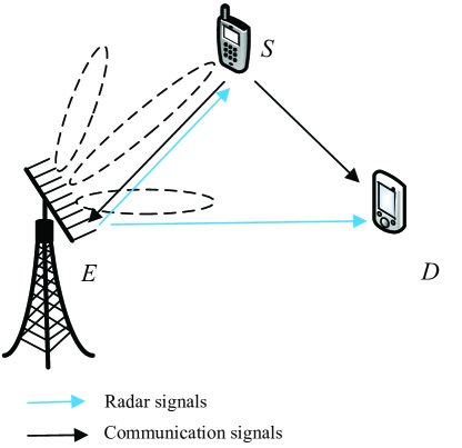
As shown in Fig. 1, we consider a JTSAPE system consists of a single-antenna illegal transmission source node , a single-antenna destination node , and a multi-antenna BS . There is an illegal link for adaptive transmission between and [24], [25], [26], and transmits signals to detect and eavesdrops the information that sends to . It is assumed that is equipped with uniform linear array (ULA) antennas with transmitting and receiving antennas and the angle of is known a priori based on the results of the detection stage, like many works [18], [20].
The objective of this work is to estimate the target parameter and implement proactive eavesdropping. To evaluate the estimation accuracy, the CRB and the eavesdropping SINR are evaluated as the performance metrics of the radar and proactive eavesdropping, respectively.
II-A The Radar Model
The transmitted signal, , at is expressed as
| (1) |
where is the transmit beamformer to be designed, denotes the symbols with unit power. It assumes that the data symbols are approximately orthogonal to each other, which denotes .
Like [12, 22], since the radar host generally has a strong signal separation capability, and a variety of methods can be used for filtering. Then, is assumeded that can completely separate the signal and eliminate the noise. When there are targets, the echo received by the radar is expressed as
| (2) |
where , , , , , and , and are the steering vector of the transmitting and receiving arrays, is the antenna spacing, denotes the wavelength, is the angle of the target when the first antenna is utilized as the reference point, is noise power, the normalized parameter depends on the complex amplitude of the target reflection and path loss coefficient of the link. According to (2), . The Fisher information matrix (FIM) of a vector is expressed as
| (3) |
where and denote the covariance matrix and mean vector [27]. In this work, the target direction , the real and imaginary parts of the coefficient are estimated. Since is independent of the estimator [8, 21, 30], therefore, the FIM for is given in the following Lemma.
Lemma 1.
The FIM for is expressed as
| (7) |
where , , , , , and .
In this work, it is assumed that there is one target. The singal target echo sensing signal received by is expressed as [19]
| (8) |
where is the additive white Gaussian noise (AWGN) matrix.
Proof.
Please refer to Appendix A. ∎
The CRB matrix is obtained as
| (9) |
II-B The Proactive Eavesdropping Model
It is assumed that a radar signal is used as AN to realize proactive eavesdropping, and the line-of-sight channel between and is expressed as [18]
| (10) |
where represents the channel gain at the reference distance, represents the distance between and , and represents the path loss exponent. The channel between and is expressed as
| (11) |
where represents the distance between and . The radar signal transmitted from also acts as an AN singnals to reduce the illegal link transmission rate. Thus, the received signal at is expressed as
| (12) |
where denotes the signal sent by , and is the AWGN. The SNR of received signal at is expressed as
| (13) |
where is the transmit power of , and signifies the beampattern from .
The communication signals received at is expressed as
| (14) |
where , is the channel. It is assumed that adopts the selection combining scheme, the SNR of is expressed as
| (15) |
where , represents the distance between and .
III Problem Formulation
In this section, we first consider the covariance matrix design for proactive eavesdropping and target sensing, respectively. Then, the joint optimization of proactive eavesdropping and target sensing is considered. A normalized weighted optimization problem is proposed to examine the trade-off between the target parameter estimation and proactive eavesdropping.
III-A Proactive Eavesdropping Only
In this work, it is assumed that there is an adaptive information transmission link between and , can decode the received information without error, and the success of proactive eavesdropping needs to meet [24, 25, 26]. In this subsection, proactive eavesdropping is considered only, which indicates that the transmitting beam is designed to meet the eavesdropping demand. The problem of proactive eavesdropping is formulated as
| (16a) | ||||
| (16b) | ||||
| (16c) | ||||
| (16d) | ||||
where (16a) is the premise of successful eavesdropping, (16b) is the constraint on the total power, where denotes the power budget of , (16c) indicates that the covariance matrix is a positive semi-definite matrix, and (16d) indicates that the rank of is one.
is challengeable to solve because the convexity of (16a) is unknown and (16d) is non-convex. By substituting (13) and (15) into (16a), which is rewritten as
| (17) |
Based on (13), it can be found that maximing equals to minimizing . Then, is equivalent to
| (18a) | ||||
| (18b) | ||||
| (18c) | ||||
| (18d) | ||||
where is non-negative. With the same method as [16], igoring (18d), can be solved directly by the convex optimization toolbox.
III-B Target Sensing Only
CRB is the lower bound of the unbiased estimation variance, and therefore minimizing CRB is a strategy for improving the accuracy of the estimation. In this subsection, target sensing is considered only, which indicates that the transmitting beam is designed to minimize the CRB.
III-B1 Pefect Target Direction
In this subsection, it is assumed that the given target angle is perfect. The formulated problem is expressed as
| (19a) | ||||
| (19b) | ||||
| (19c) | ||||
| (19d) | ||||
where denotes the direction of , prescribes the sidelobe region, the left-hand side (LHS) of (19a) is the difference between the gain of the target direction and the gain of other directions, represents other angles in the detection range except the target angle , and is the constant threshold. The purpose of (19a) is to ensure that the gain in the target direction is superior to that in the other directions. The objective function of is to minimize the determinant of , which conforms to the convex limit. is a standard SDR problem after ignoring the rank-1 constraint and can be solved by CVX toolbox.
III-B2 Impefect Target Direction
In this subsection, more practical scenario is considered wherein the given target angle is imperfect and there is an uncertain angle . Specifically, the angle of the radar’s main detection is changed in . Then, the following optimization problem is formulated
| (20a) | ||||
| (20b) | ||||
| (20c) | ||||
| (20d) | ||||
| (20e) | ||||
| (20f) | ||||
where represents other angles except the main lobe direction, is constraint constant, . (20a) represents the gain gap threshold constraint between the target direction and side lobes, (20b) and (20c) are both stable mainlobe gain intervals to prevent a large gain difference which affects the detection performance. under an uncertain target sensing angle can be solved by CVX after ignoring (20f).
III-C Jointly Optimization of Proactive Eavesdropping and Target Sensing
In this section, a normalized weighted optimization problem that reveals the performance tradeoff between proactive eavesdropping and target sensing is proposed. The design of a weighted optimization between the radar CRB and the eavesdropping rate presents the challenge that the two performance metrics have different units and potentially different magnitudes. Inspired by [21], the CRB and the eavesdropping rate are normalized with their respective bound obtained in and , respectively.
III-C1 Joint Optimization Proactive Eavesdropping and Target Sensing
To achieve a tradeoff between the eavesdropping performance and the target sensing, while taking the uncertain angle of into account, the weighted optimization problem is formulated as
| (21a) | ||||
| (21b) | ||||
| (21c) | ||||
| (21d) | ||||
| (21e) | ||||
| (21f) | ||||
| (21g) | ||||
where is the result of the optimization problem , is the result of the optimization problem , and signifies the factor that determines the proactive eavesdropping and target sensing performance weights, .
is an SDR problem by neglecting (21e), and the CVX toolbox can be utilized to solve the problem. The above-solving process is summarized as Algorithm 1.
III-C2 The interference power is zero
It is unnecessary for to send noise to when the channel quality of is better than that of , i.e. in (21d) [29]. In these scenarios, the eavesdropping rate is equal to the receiving rate of without interference and is transformed into a target sensing sub-problem, which is expressed as
| (22a) | ||||
| (22b) | ||||
| (22c) | ||||
| (22d) | ||||
| (22e) | ||||
| (22f) | ||||
| (22g) | ||||
where (22a) denotes the interference from at equal to zero.
is a standard convex problem when (22d) is omitted, which can be solved directly by CVX. The solving process is summarized as Algorithm 2.
III-C3 The Rank-1 Constraint
The rank-1 constraint is non-convex, which means the optimization problem can not be directly solved by the relevant toolbox. The above problems are solved by omitting the rank-1 constraint and the rank of the obtained solution may be larger than one.
Based on Refs. [16] and [21], the feasible suboptimal solution of the original problem can be obtained by utilizing specific methods based on the SDR technology, and rank-1 constraint is solved by Gaussian randomization or singular value decomposition, etc. It must be noted that these methods may result in a certain degree of distortion, which is tolerable in many cases. However, these methods cannot be applied to our system model since the recovered result may not satisfy , which results in failure eavesdropping.
For the obtained solution with , an iterative method is utilized, which is expressed as
| (23) |
where denotes the diagonal matrix composed of eigenvalues and is the eigenvector matrix. Firstly, the eigenvalue matrix is obtained by eigenvalue decomposition. According to the relationship between the matrix eigenvalue and the matrix trace, the maximum eigenvalue of must be less than the trace. The eigenvector of maximum eigenvalue of is expressed as and there must be . Let , by using the iterative method, the rank-1 constraint is transformed into
| (24) |
where denotes -th iteration value. Then and are reformulated as
| (25a) | ||||
| (25b) | ||||
| (25c) | ||||
| (25d) | ||||
| (25e) | ||||
| (25f) | ||||
| (25g) | ||||
| (25h) | ||||
and
| (26a) | ||||
| (26b) | ||||
| (26c) | ||||
| (26d) | ||||
| (26e) | ||||
| (26f) | ||||
| (26g) | ||||
| (26h) | ||||
respectively. The initial value of is obtained by solving , and . The optimal result of is denoted as in -th iteration, which are solved by an iterative algorithm summarized as Algorithm 3. After obtain by solving , the beamforming vector, , is obtained through the eigenvalue decomposition.
IV Numerical Results and Discussion
In this section, simulation results are presented to prove the convergence and effectiveness of our algorithm. The positions of , , and are expressed as , , and , respectively. The positive direction of the X axis is used as the reference direction, and the azimuth angles of and relative to are expressed as and , respectively. The direction of the radar detection range is , radar resolution of 1 degrees, , and other parameters are listed in Table I. In all the simulation figures, ‘PEO,’ ‘TSO,’ and ‘JPT’ correspond to the results for proactive eavesdropping only, target sensing only, and joint optimization of proactive eavesdropping and target sensing, respectively.
| Parameters | Value | Parameters | Value |
| -30 dB | |||
| -80 dBm | 0.05 | ||
| 0.01 | 2.7 | ||
| 30 dBm | |||
| 0.999 | 12 | ||
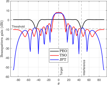
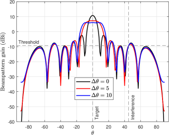
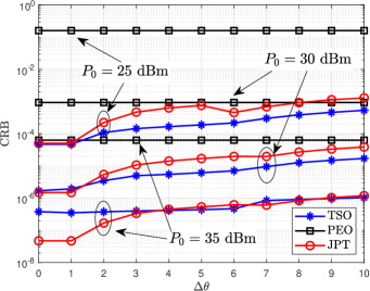
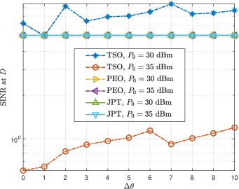
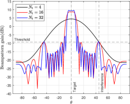
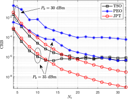
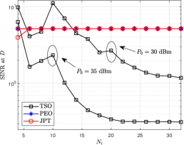
Fig. 2(a) shows the beampattern gain with different schemes. It can be observed that, in PEO scheme where only active eavesdropping is carried out, in the direction where is located , the beampattern gain needs to meet the corresponding threshold to reduce the received SINR of because the quality of eavesdropping channel is worse than that of -. In the TSO scheme where only the target sensing is considered, the beampattern gain is highest in the direction of the sensing target . In JPT, where proactive eavesdropping and target sensing are considered simultaneous, the direction of needs to have the highest beampattern gain, and the direction of must meet the threshold requirement. Fig. 2(b) plots the beam gain corresponding to the uncertainty with the JPT scheme. We can find that when the target angle is perfect , the main lobe of the beam is the narrowest. With the increase of , the main lobe width becomes more expansive and the gain decreases because the energy is spread over a larger area. However, in the direction of , the gain must be not less than the requirement. Fig. 2(c) demonstrates the CRB versus varying under different schemes. The CRB of PEO is impendent to since only proactive eavesdropping is considered. When target sensing is taken into account, the CRB increases with the increase of the uncertainty angle because the main lobe widens, and the beam gain decreases. As increases, the CRB of JPT is gradually lower than TSO when the target angle is perfect , indicating that the estimation effect of JPT is more accurate. This is because the constraint in the ’s direction increases the main lobe gain. In the high- region, the CRB of TSO is lower than that of JPT because the energy allocated to the direction gradually decreases with the increase of and the beam gain decreases. In addition, when the transmitting power of the radar increases dBm, the corresponding CRB decreases because the transmitting power of the radar is high, and the gain in the ’s direction is also increased. Fig. 2(d) plots the versus varying with different schemes. We can find that, since proactive eavesdropping is not considered in the TSO scheme, the beam gain in ’s direction may be less than the threshold when is lower, resulting in eavesdropping failure. On the contrary, with the higher , the gain in ’s direction is greater than the threshold, and the eavesdropping is successful, but the eavesdropping SINR is relatively low. The ’s SINR of the PEO and JPT schemes is a constant, which denotes that successful eavesdropping is achieved and the maximum eavesdropping rate is obtained.
Fig. 3(a) shows the relationship between beam gain and of the JPT scheme. The results show that the resolution of beam gain increases with increasing . The main lobe gain also increases because the ability to control the energy distribution increases. Fig. 3(b) demonstrates the relationship between the CRB and of the JPT scheme. The CRB decreases with the increase of , which signifies that the sensing accuracy increases. This is because the main lobe gain increases as increases. Fig. 3(c) plots the SINR at for different schemes versus varying . It is observed that the TSO scheme gradually succeeds in eavesdropping, and eavesdropping SINR decreases with the increase of since only target sensing is considered.
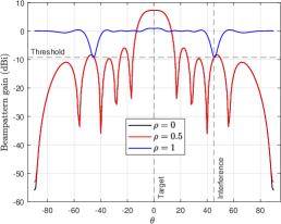
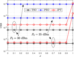
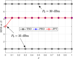
Fig. 4(a) shows the beam gain of the JPT scheme with varying . As shown in the figure, when , the JPT scheme degenerates into the PEO scheme, but there is a small main lobe in the ’s detection because JPT introduces constraints on the gain of the main lobe. Fig. 4(b) plots the relationship between CRB and for different schemes. The CRB with is the largest because of the same reason of Fig. 4(a). Because the energy of the main lobe is independent of the , the CRB is a constant. The CRB of TSO is better than that of JPT because the gain constraint in the direction is absent. Fig. 4(c) plots the versus varying with different schemes. When and dBm, the JPT scheme eavesdropping is successful but the eavesdropping rate is low because the JPT scheme degenerates into the TSO scheme with and the gain in ’s direction is greater than the threshold.
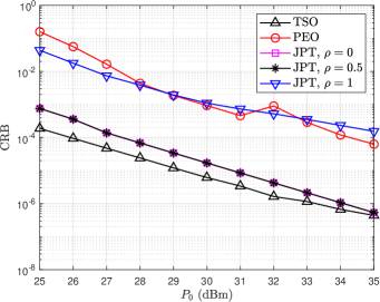
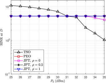
Fig. 5(a) demonstrates the relationship between CRB and radar power budget for various schemes. It can be observed that the CRB decreases linearly with the increase of , which denotes that increasing the power budget can improve the accuracy of sensing. The CRB of the TSO scheme tends to be constant in the high- region, indicating that when the transmitting power reaches a certain level, simply increasing the transmitting power cannot improve the sensing accuracy. Fig. 5(b) plots the of various schemes versus the varying . The of the TSO scheme decreases with the increase of because only the target sensing is considered, the gain in the direction of the illegal receiver is not constrained, and no proactive eavesdropping is carried out. When , the eavesdropping SINR of the JPT scheme also decreases with the increasing because the JPT scheme degenerates into the TSO scheme. The eavesdropping SINR of PEO and JPT schemes with non-zero is a constant, which signifies proactive eavesdropping also is successfully performed.
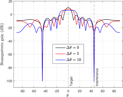
Fig. 6 plots the beam gain when the interference power is equal to zero. At this time, because the quality of the eavesdropping channel is better than that of the illegal communication channel, it is not necessary to transmit power in ’s direction.
V Conclusion
This paper studied proactive eavesdropping in the JTSAPE system wherein the multi-antenna BS transmits the signal to realize target sensing which was utilized as AN to realize proactive eavesdropping. Two waveform design schemes were proposed to maximize the eavesdropping SNR or minimize the CRB, respectively. Then, a normalized weighted optimization problem was formulated to optimize proactive eavesdropping and target sensing jointly. After omitting the Rank-1 constraint, the non-convex problem was solved by the SDR technique. The SROCR method is utilized to solve continuously and iteratively to obtain Rank-1 beamforming solution.
Appendix A Proof of Lemma 1
Based on (3), the FIM for is expressed as
| (30) |
wherein each of the elements is a matrix. In particular, the first element is expressed as
| (34) |
where is expressed as
| (35) |
where , denotes the element of the matrix , denotes the -th column of the identity matrix, step holds by following
| (36) |
step holds by following
| (37) |
and step holds by following
| (38) |
With some simple algebraic manipulations, the element of is expressed as
| (39) |
where and .
The element of is expressed as
| (40) |
where and .
The element of is expressed as
| (41) |
The element of is expressed as
| (42) |
The element of is expressed as
| (43) |
The element of is expressed as
| (44) |
The element of is expressed as
| (45) |
The element of is expressed as
| (46) |
References
- [1] F. Liu, Y. Cui, C. Masouros, J. Xu, T. X. Han, Y. C. Eldar, and S. Buzzi, “Integrated sensing and communications: Towards dual-functional wireless networks for 6G and beyond,” IEEE J. Sel. Areas Commun., vol. 40, no. 6, pp. 1728-1767, Jun. 2022.
- [2] F. Dong, F. Liu, Y. Cui, W. Wang, K. Han, and Z. Wang, “Sensing as a service in 6G perceptive networks: A unified framework for ISAC resource allocation,” IEEE Trans. Wireless Commun., vol. 22, no. 5, pp. 3522-3536, May 2023.
- [3] Z. Wei, H. Qu, Y. Wang, X. Yuan, H. Wu, Y. Du, K. Han, N. Zhang, and Z. Feng, “Integrated sensing and communication signals toward 5G-A and 6G: A survey,” IEEE Internet Things J., vol. 10, no. 13, pp. 11068-11092, Jul. 2023.
- [4] Z. Wei, F. Liu, C. Masouros, N. Su, and A. P. Petropulu, “Toward multi-functional 6G wireless networks: Integrating sensing, communication, and security,” IEEE Commun. Mag., vol. 60, no. 4, pp. 65-71, Apr. 2022.
- [5] F. Liu, Y.-F. Liu, A. Li, C. Masouros, and Y. C. Eldar, “Cramér-Rao bound optimization for joint radar-communication beamforming,” IEEE Trans. Signal Process., vol. 70, pp. 240 - 253, Dec. 2022.
- [6] X. Li, F. Liu, Z. Zhou, G. Zhu, S. Wang, K. Huang, and Y. Gong, “Integrated sensing, communication, and computation over-the-air: MIMO beamforming design,” IEEE Trans. Wireless Commun., vol. 22, no. 8, pp. 5383-5398, Aug. 2023.
- [7] C. Wen, Y. Huang, L. Zheng, W. J. Liu, and T. N. Davidson, “Transmit waveform design for dual-function radar-communication systems via hybrid linear-nonlinear precoding,” IEEE Trans. Signal Process., vol. 71, pp. 2130-2145, Jun. 2023.
- [8] Z. Ren, Y. Peng, X. Song, Y. Fang, L. Qiu, L. Liu, D. W. K. Ng, and J. Xu, “Fundamental CRB-rate tradeoff in multi-antenna ISAC systems with information multicasting and multi-target sensing,” IEEE Trans. Wireless Commun., vol. 23, no. 4, pp. 3870-3885, Apr. 2024.
- [9] Z. Zhao, L. Zhang, R. Jiang, X.-P. Zhang, X. Tang, and Y. Dong, “Joint beamforming scheme for ISAC systems via robust Cramér–Rao bound optimization,” IEEE Wireless Commun. Lett., vol. 13, no. 3, pp. 889-893, Mar. 2024.
- [10] T. Liu, Y. Guo, L. Lu, and B. Xia, “Waveform design for integrated sensing and communication systems based on interference exploitation,” J. Commun. Inform. Netw., vol. 7, no. 4, pp. 447-456, Dec. 2022.
- [11] Y. Guo, Y. Liu, Q. Wu, X. Li, and Q. Shi, “Joint beamforming and power allocation for RIS aided full-duplex integrated sensing and uplink communication system,” IEEE Trans. Wireless Commun., vol. 23, no. 5, pp. 4627-4642, May 2024.
- [12] Z. He, W. Xu, H. Shen, D. W. K. Ng, Y. C. Eldar, and X. You, “Full-duplex communication for ISAC: Joint beamforming and power optimization,” IEEE J. Sel. Areas Commun., vol. 41, no. 9, pp. 2920-2936, Sep. 2023.
- [13] R. Liu, M. Li, Q. Liu, and A. L. Swindlehurst, “SNR/CRB-constrained joint beamforming and reflection designs for RIS-ISAC systems,” IEEE Trans. Wireless Commun., doi: 10.1109/twc.2023.3341429, 2023.
- [14] H. Hua, T. X. Han, and J. Xu, “MIMO integrated sensing and communication: CRB-rate tradeoff,” IEEE Trans. Wireless Commun., vol. 23, no. 4, pp. 2839-2854, Apr. 2024.
- [15] G. Wu, Y. Fang, J. Xu, Z. Feng, and S. Cui, “Energy-efficient MIMO integrated sensing and communications with on-off non-transmission powers,” IEEE Internet Things J., vol. 11, no. 7, pp. 12177-12191, Apr. 2024.
- [16] N. Su, F. Liu, and C. Masouros, “Secure radar-communication systems with malicious targets: Integrating radar, communications and jamming functionalities,” IEEE Trans. Wireless Commun., vol. 20, no. 1, pp. 83-95, Jan. 2021.
- [17] N. Su, F. Liu, Z. Wei, Y.-F. Liu, and C. Masouros, “Secure dual-functional radar-communication transmission: Exploiting interference for resilience against target eavesdropping,” IEEE Trans. Wireless Commun., vol. 21, no. 9, pp. 7238-7252, Sept. 2022.
- [18] H. Jia, X. Li, and L. Ma, “Physical layer security optimization with Cramér-Rao bound metric in ISAC systems under sensing-specific imperfect CSI model,” IEEE Trans. Veh. Technol., doi: 10.1109/tvt.2023.3347527, Jun. 2023.
- [19] F. Dong, W. Wang, X. Li, F. Liu, S. Chen, and L. Hanzo, “Joint beamforming design for dual-functional MIMO radar and communication systems guaranteeing physical layer security,” IEEE Trans. Green Commun. Netw., vol. 7, no. 1, pp. 537-549, Mar. 2023.
- [20] Z. Ren, L. Qiu, J. Xu, and D. W. K. Ng, “Robust transmit beamforming for secure integrated sensing and communication,” IEEE Trans. Commun., vol. 71, no. 9, pp. 5549-5564, Sep. 2023.
- [21] N. Su, F. Liu, and C. Masouros, “Sensing-assisted eavesdropper estimation: An ISAC breakthrough in physical layer security,” IEEE Trans. Wireless Commun., vol. 23, no. 4, pp. 3162-3174, Apr. 2024.
- [22] J. Chu, R. Liu, M. Li, Y. Liu, and Q. Liu, “Joint secure transmit beamforming designs for integrated sensing and communication systems,” IEEE Trans. Veh. Technol., vol. 72, no. 4, pp. 4778-4791, Apr. 2023.
- [23] J. Zhang, J. Xu, W. Lu, N. Zhao, X. Wang, and D. Niyato, “Secure tansmission for IRS-aided UAV-ISAC networks,” IEEE Trans. Wireless Commun., doi: 10.1109/twc.2024.3390169, 2024.
- [24] F. Feizi, M. Mohammadi, Z. Mobini, and C. Tellambura, “Proactive eavesdropping via jamming in full-duplex multi-antenna systems: Beamforming design and antenna selection,” IEEE Trans. Commun., vol. 68, no. 12, pp. 7563-7577, Dec. 2020.
- [25] D. Xu and H. Zhu, “Jamming-assisted legitimate eavesdropping and secure communication in multicarrier interference networks,” IEEE Syst. J., vol. 16, no. 1, pp. 954-965, Mar. 2022.
- [26] G. Hu, Z. Li, J. Si, K. Xu, Y. Cai, D. Xu, and N. Al-Dhahir, “Analysis and optimization of STAR-RIS-assisted proactive eavesdropping with statistical CSI,” IEEE Trans. Veh. Technol., vol. 72, no. 5, pp. 6850-6855, May 2023.
- [27] S. M. Kay, Fundamentals of Statistical Signal Processing: Estimation Theory. Englewood Cliffs, NJ: Prentice-Hall, Inc., 1993.
- [28] I. Bekkerman and J. Tabrikian, “Target detection and localization using MIMO radars and sonars,” IEEE Trans. Signal Process., vol. 54, no. 10, pp. 3873-3883, Oct. 2006.
- [29] X. Jiang, H. Lin, C. Zhong, X. Chen, and Z. Zhang, “Proactive eavesdropping in relaying systems,” IEEE Signal Process. Lett., vol. 24, no. 6, pp. 917-921, Jun. 2017.
- [30] J. Li, L. Xu, P. Stoica, K. W. Forsythe, and D. W. Bliss, “Range compression and waveform optimization for MIMO radar: A Cramér–Rao bound based study,” IEEE Trans. Signal Process., vol. 56, no. 1, pp. 218-232, Jan. 2008.