Benchmarks for quantum computers from Shor’s algorithm

The rapid development of quantum technologies over the last decade has prompted much research on techniques for checking that the carefully engineered quantum devices are, in fact, functioning properly [1, 2, 3]. In the survey of the field presented in [2], a distinction is drawn between certification (or verification) and benchmarking. Certification is taken to be confined to the assessment the accuracy of the output, whereas benchmarking protocols are any more general measures of performance. Clearly, in this parlance, Shor’s factoring algorithm and the associated period-finding algorithm can be used for verification as the validity of their output is easily checked, but the ancillary properties mentioned in the abstract and discussed below could serve as the basis for benchmarks that test circuits as a whole.

In Shor’s version of his factoring algorithm [4], a square-free semiprime $N$ is factored by first using a quantum computer to determine the order $r$ of an arbitrary element $b\in(\mathbb{Z}/N\mathbb{Z})^{\times}$, or, more colloquially, the period of $b^{x}\mathrm{mod}\,N$, and then using a classical computer to calculate the candidate $f_{b}=\gcd(b^{r/2}-1,N)$ for a non-trivial factor of $N$. (Unless specified otherwise, the notation of [5] is adopted.)

It is the dependence on the period $r$ of the probability for success of the period-finding algorithm which is relevant to benchmarking. The nature of this dependence can be established by considering the sequence of input register sizes $\{\mathfrak{m}_{\mathfrak{q}}\}$, where $\mathfrak{m}_{\mathfrak{q}}$ is the smallest positive integer such that

and $\mathfrak{q}$ is any integer consistent with the requirement that the input register is large enough for the quantum Fourier transform of its state to yield information on $r$, i.e. $2^{\mathfrak{m}_{\mathfrak{q}}}\geq 2r$ from the $k=r-1$ version of the first inequality in (5), or $\mathfrak{q}\geq\mathfrak{q}_{\min}=\lceil\log_{2}r\rceil-\lfloor 2\log_{2}r\rfloor$.

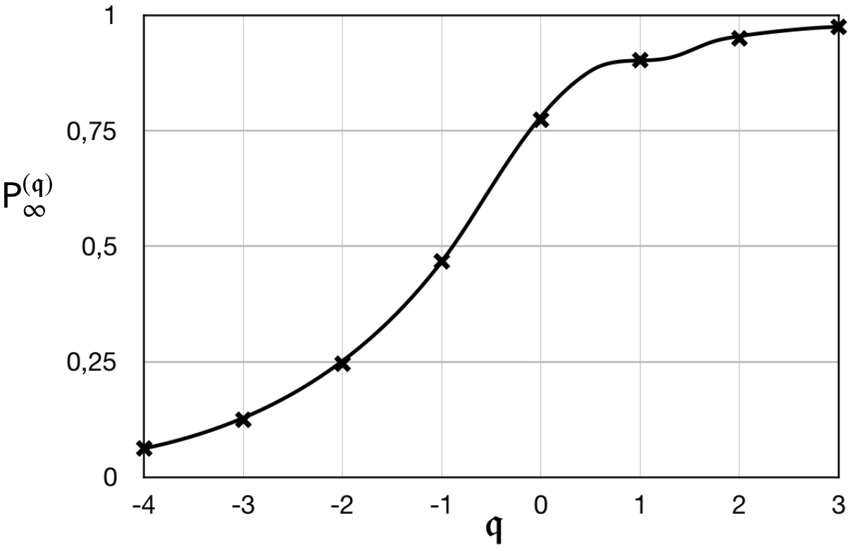
A systematic asymptotic analysis implies that, when $r\gg 1$, a useful approximation to the probability of finding a divisor of $r$ (or $r$ itself) with an input register of $\mathfrak{m}_{\mathfrak{q}}$ qubits is

($\operatorname{Si}(x)$ is the sine integral of Eq. 6.2.9 in [6]). The monotonically increasing sequence $\{\mathsf{P}^{(\mathfrak{q})}_{\infty}\}$ is depicted in Fig. 1. The interpolating curve is obtained with the same function used to evaluate the $\mathsf{P}^{(\mathfrak{q})}_{\infty}$’s. As the derivation of section 2 and (28) make clear, the result in (2) pertains to the determination of the period of any function of the integers $\mathbb{Z}$ provided it is one-to-one within a period, and the period $r$ is not a divisor of $2^{\mathfrak{m}_{\mathfrak{q}}}$. When $r$ is a power of two (and, hence, a divisor of $2^{\mathfrak{m}_{\mathfrak{q}}}$), the probability of success is independent of $\mathfrak{q}$ [see (28)].

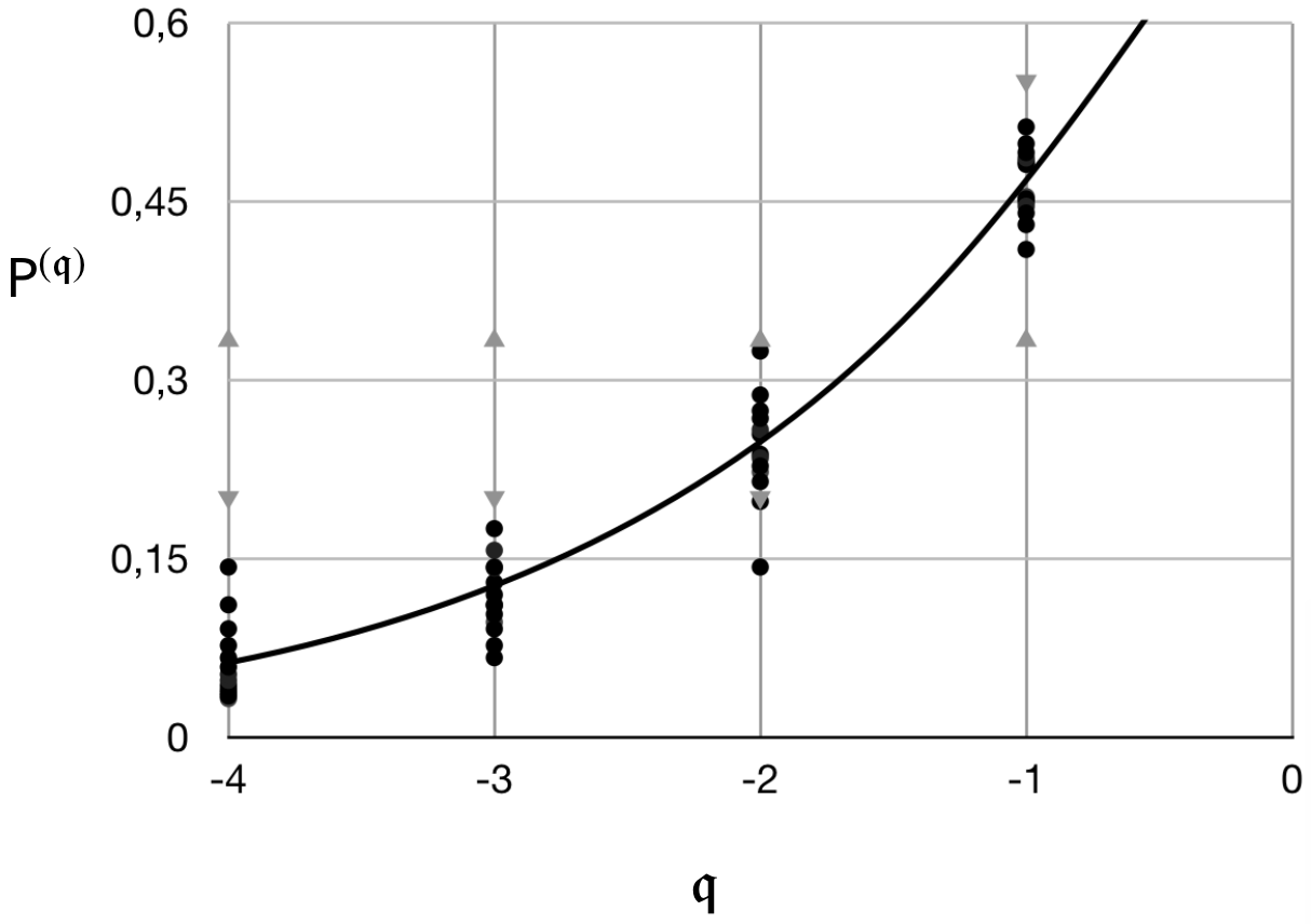
The register of $\mathfrak{m}_{0}=\lceil 2\log_{2}r\rceil$ qubits is distinguished by the fact that it is, generically, the smallest for which $\mathsf{P}^{(\mathfrak{q})}_{\infty}$ exceeds 50%. Among the inferences that one can draw from Fig. 1 is that the magnitude of the probability of success for the period-finding algorithm amounts to a fingerprint of the critical input register. Statistics on the success or failure of runs for $\mathfrak{m}_{0}$ qubits would permit empirical determination of the corresponding probability of success of the period-finding algorithm; unambiguous comparison of the probability found with $\mathsf{P}^{(\mathfrak{q=0})}_{\infty}$ should be possible in view of its clear separation in value from the other $\mathsf{P}^{(\mathfrak{q})}_{\infty}$’s: this comparison constitutes the first benchmark, applicable whenever $r$ is not a divisor of $2^{\mathfrak{m}_{0}}$ (as is typically the case).

Corrections to $\mathsf{P}_{\infty}^{(\mathfrak{q})}$, considered in section 3, do not invalidate any of the observations above. In fact, it is found that, for $\mathfrak{q}\geq 0$, these corrections are negligible (see (30), (31) and Table 2). The clear difference between the success probability for the critical input register and input registers of other sizes also survives (see Fig. 3).

Another opportunity for benchmarking is provided by the choice of the element $b\in(\mathbb{Z}/N\mathbb{Z})^{\times}$. Leander has pointed out [7] that if $b$ is selected so that the Jacobi symbol $(b/N)=-1$ (“Choice L”), then, not only is the order $r$ of $b$ guaranteed to be even, but also the probability that $f_{b}=\gcd(b^{r/2}-1,N)$ is a non-trivial factor of $N$ is enhanced; for $r$ even, $f_{b}$ is the desired factor provided $b^{r/2}\not\equiv-1(\mathrm{mod}\,N)$: the conditional probability

where the positive integer powers $c_{p}\geq c_{q}$ are related to the square-free semiprime $N$ by the parametrisation $N=(2^{c_{p}}d_{p}+1)(2^{c_{q}}d_{q}+1)$, it being understood that $d_{p}$ and $d_{q}$ are, by definition, odd. The success rate of the prescription for $f_{b}$ is at least 75% as compared with 50% if $b$ is chosen at random from $(\mathbb{Z}/N\mathbb{Z})^{\times}$, but this observation does not do justice to the full implications of (1).

The crux to building on Leander’s criterion for $b$ is to recognise that, in principle, it can only fail to generate a factor of $N$ if $c_{p}>c_{q}$. When it is known that $c_{p}>c_{q}$, then $b$ should be a quadratic non-residue modulo $N$ for which $(b/N)=+1$ (“Choice $\overline{\mathrm{L}}$”); the corresponding probability that $f_{b}$ is a prime factor of $N$ is $1-\delta_{c_{p},c_{q}}$: if $c_{p}>c_{q}$, $f_{b}$ must then be a non-trivial factor of $N$. (As for choice L, the fact that $b$ is a quadratic non-residue ensures that its order is even.)

There are two clear-cut complementary benchmarking schemes $\mathcal{A}$ and $\mathcal{B}$: scheme $\mathcal{A}$ ($\mathcal{B}$) entails determination of the probability that $\overline{\mathrm{L}}$-choices (L-choices) for $b$ do actually yield a prime factor of $N$ given that $c_{p}>c_{q}$ ($c_{p}=c_{q}$). Identification of whether $c_{p}>c_{q}$ or $c_{p}=c_{q}$ requires successful factorization of $N$, which can be achieved with a suitable sequence of initial runs, beginning with a few L-choices, and converting to $\overline{\mathrm{L}}$-choices if these runs fail. For both $\mathcal{A}$ and $\mathcal{B}$, the empirical probability is to be compared with a predicted value of unity. The overhead placed on classical computer resources by the selection of appropriate values of $b$ is acceptable: calculation of the Jacobi symbols is efficient, as is checking that a given $b\in(\mathbb{Z}/N\mathbb{Z})^{\times}$ is a quadratic non-residue.

Application of the benchmarking procedures $\mathcal{A}$ and $\mathcal{B}$ should be preceded by determination of $(-1/N)$ and $(2/N)$. Provided $-1$ and 2 are quadratic non-residues modulo $N$, the values of these two Jacobi symbols permit one to infer whether $c_{p}=c_{q}$ or $c_{p}>c_{q}$ for all semiprimes such that $c_{q}\leq 2$ — see Table 1. The import of Table 1 is that, for these semiprimes, the choice between $\mathcal{A}$ and $\mathcal{B}$ can be made before the order-finding algorithm is run. Blum integers are among the semiprimes to which the results of Table 1 apply.

It remains to justify the assertions made in this introduction. The exact reduction of the success probability associated with the period-finding algorithm to a form in (2.3) suitable for controlled approximation is presented in section 2, followed by its asymptotic analysis for large $r$ using the Euler-Maclaurin summation formula in section 3. Properties of choices L and $\overline{\mathrm{L}}$ are proven in section 4, and some closing comments are made in section 5. Appendices A, B and C contain technical results required in sections 2 and 3.

After the usual preparatory steps (outlined, for example, in Algorithm 5 of Ref. [5]), an $m$-qubit input register is left in the superposition of computational basis states

where $k\in\mathbb{Z}/r\mathbb{Z}$ is unknown (and unknowable), and the constraint on $m$ that

guarantees that the superposition contains more than one term and, hence, that $S_{k}(x)$ in (7) can manifest dependence on $r$. Since

where $n_{r}$ is a non-negative integer, an implication of (5) found useful below is that $m>n_{r}$.

Interpretation of the quantum Fourier transform of the one-dimensional “array” of uniformly spaced “atoms” in (4) is possible via its “structure factor”

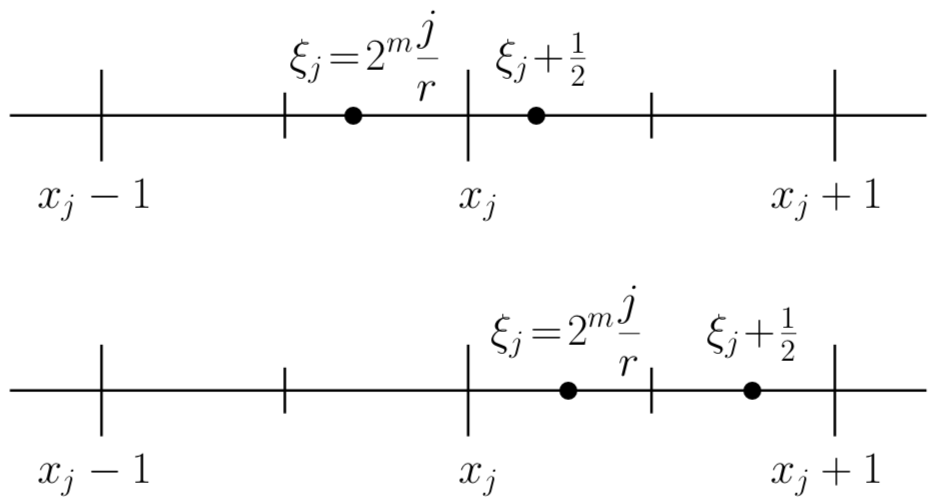
which is related to the conditional probability $P(x|k)$ that the transform is detected in the state $|x\rangle$ by $P(x|k)=S_{k}(x)/2^{m}$. Central to the standard analysis of $P(x|k)$ is the observation that, for non-zero integers $x$, $S_{k}(x)$ is large ($\sim m_{k}$) when the rational number $rx/2^{m}$, which must lie in the closed interval $[r/2^{m},r(1-1/2^{m})]$, is close to one of the $r-1$ integers $j$ in this interval, i.e.

Thus, the “frequencies” $x$ most likely to be returned by measurement are drawn from the set of integers $\{x_{j}\}$ closest to the first $r-1$ members of the harmonic series with fundamental “frequency” $2^{m}/r$:

where the inequality is strict because $2^{m}\,j/r=2^{m-n_{r}}\,j/r_{\mathrm{o}}$ can never be a half-integer. The solution of (9) is

as inspection of Fig. 2 confirms.

Equation (9) acquires additional significance if viewed from the perspective of rational approximation with continued fractions. Provided the input register size is such that $2^{m/2}>r$, then one of the finite number of convergents to $x_{j}/2^{m}$ coincides with the ratio $j/r$ reduced to lowest terms; if $m=\mathfrak{m}_{0}$, then the only observed values of $x$ from which information of this nature can be inferred are precisely those belonging to the set $\{x_{j}\}$: the total probability for success of the period-finding algorithm is

More generally, when $m=\mathfrak{m}_{\mathfrak{q}}$, the restriction on useful values of $x$ reads

When $\mathfrak{q}\geq 1$, there are $2^{\mathfrak{q}}-1$ or $2^{\mathfrak{q}}$ solutions of (12) dependent on whether $r_{\mathrm{o}}$ divides $j$ or not ($j\in\mathbb{N}_{r}^{+}$); if $\mathfrak{q}<0$, then the solutions are a subset of the $x_{j}$’s.

If $r$ is a power of two (i.e.  $r_{\mathrm{o}}=1$), then $m_{k}^{(\mathfrak{q})}=2^{\mathfrak{m}_{\mathfrak{q}}}/r$, $S_{k}(x)=\delta_{x,0}\,m_{k}^{(\mathfrak{q})}$ (for integer $x$), and (2.3) reduces without approximation to

The first summation in (2.3) is dominant, and the remaining terms are suppressed by one power of $r$ or more. The same pattern is also evident in an expansion of (2.3) for large $r$ which embraces the cases in which $r$ is not a power of two. If the negligible terms of order $1/r$ and higher are discarded, then the following approximation to $P_{\mathrm{tot}}^{(\mathfrak{q})}$ emerges:

The expansions in support of (29) are given in appendix B. Like (28), (29) is independent of $k$, but, when specialized to $r_{\mathrm{o}}=1$, yields $\mathsf{P}^{(\mathfrak{q})}=1$.

Simple as the expression for $\mathsf{P}^{(\mathfrak{q})}$ is, it would seem of little utility because of its reliance on the factor $r_{\mathrm{o}}$ of the unknown (but large) period $r$. However, the numerical data in Table 2 suggests that $\mathsf{P}^{(\mathfrak{q})}$ is a monotonically decreasing function of $r_{\mathrm{o}}$ when $\mathfrak{q}\geq 0$. This trend can be confirmed for large $r_{\mathrm{o}}$ with the aid of the Euler-Maclaurin summation formula, which, for $\mathfrak{q}\geq 1$, implies straightforwardly that

The calculation is trickier for $\mathfrak{q}=0$; application of the Euler-Maclaurin summation formula has to be followed by an expansion in inverse powers of $r_{\mathrm{o}}$ (details are given in appendix C): the outcome of these manipulations is

The results in (30), (31) and Table 2 justify the claim that, provided $1/r$ is negligible, $\mathsf{P}^{(\mathfrak{q})}_{\infty}$ in (2) is always an excellent approximation to $P_{\mathrm{tot}}^{(\mathfrak{q})}$ in (2.3) when $\mathfrak{q}$ is non-negative.

The behaviour of $\mathsf{P}^{(\mathfrak{q})}$ for $\mathfrak{q}<0$ is quite different. Now, the expansion in inverse powers of $r_{\mathrm{o}}$, which is obtained along the same lines as (31), reads

where $\nu$ is the least non-negative residue of $r_{\mathrm{o}}$ modulo $2^{|\mathfrak{q}|+1}$. The correction to the leading term $\mathsf{P}^{(\mathfrak{q})}_{\infty}$ is of either sign and, being of order $1/r_{\mathrm{o}}$ (see Table 3), can be substantial for small $r_{\mathrm{o}}$ – see Fig. 3. Despite the scatter about $\mathsf{P}^{(\mathfrak{q})}_{\infty}$ in the values of $\mathsf{P}^{(\mathfrak{q})}$ for $\mathfrak{q}<0$, none are close to $\mathsf{P}^{(0)}$.

The leading term $\mathsf{P}^{(\mathfrak{q})}_{\infty}$ in all of the above expansions in (30), (31) and (32) is found by evaluation of

for integer $\mathfrak{q}$. The integral in (33) defines an entire function of $z=2^{\mathfrak{q}}$. In the limit $r_{\mathrm{o}}\rightarrow\infty$, when $\mathsf{P}^{(\mathfrak{q})}\rightarrow\mathsf{P}^{(\mathfrak{q})}_{\infty}$, the lower limit on the integers $\mathfrak{q}$ of $\mathfrak{q}_{\min}\rightarrow-\infty$; the values of $2^{\mathfrak{q}}$ then belong to a set with an accumulation point, and the identity theorem for holomorphic functions can be invoked to assert that the integral representation in (33) is the unique analytic continuation of $\mathsf{P}^{(\mathfrak{q})}_{\infty}$ to all values of $\mathfrak{q}$, real and complex: thus, the right-hand side of (2), which is obtained from (33) for arbitrary $\mathfrak{q}$ by integration by parts, is a natural choice of interpolation function in Fig. 1.

Insight into good choices of $b$ for the factorization of square-free odd semiprimes $N=pq$ is gained through the isomorphism between $(\mathbb{Z}/N\mathbb{Z})^{\times}$ and the direct product $(\mathbb{Z}/p\mathbb{Z})^{\times}\times(\mathbb{Z}/q\mathbb{Z})^{\times}$ of the cyclic groups $(\mathbb{Z}/p\mathbb{Z})^{\times}$ and $(\mathbb{Z}/q\mathbb{Z})^{\times}$. The Jacobi symbol permits some consequences of this isomorphism to be recast in a manner which does not require any knowledge of the odd primes $p$ and $q$.

References

- [1] A. Gheorghiu, T. Kapourniotis and E. Kashefi, “Verification of quantum computation: an overview of existing approaches,” Theory Comput. Syst. 63, 715–808 (2019).
- [2] J. Eisert, D. Hangleiter, N. Walk, I. Roth, D. Markham, R. Parekh, U. Chabaud and E. Kashefi, “Quantum certification and benchmarking,” Nat. Rev. Phys. 2, 382–90 (2020).
- [3] M. Kliesch and I. Roth, “Theory of quantum system verification,” PRX Quantum 2, 010201 (2021).
- [4] P. W. Shor, “Polynomial time algorithms for prime factorization and discrete logarithms on a quantum computer,” SIAM J. Comput. 26(5), 1484–509 (1997).
- [5] A. M. Childs and W. van Dam, “Quantum algorithms for algebraic problems,” Rev. Mod. Phys. 82(1), 1–52 (2010).
- [6] NIST Digital Library of Mathematical Functions (Release 1.1.3 of 2021-09-15), F. W. J. Olver, A. B. Olde Daalhuis, D. W. Lozier, B. I. Schneider, R. F. Boisvert, C. W. Clark, B. R. Miller, B. V. Saunders, H. S. Cohl, and M. A. McClain (eds.).
- [7] G. Leander, “Improving the success probability of Shor’s factoring algorithm,” arXiv: quant-ph/0208183.
- [8] P. S. Bourdon and H. T. Williams, “Sharp probability estimates for Shor’s order-finding algorithm,” Quantum Information & Computation 7(5&6), 522–50 (2007).
- [9] G. H. Hardy and E. M. Wright, “An introduction to the theory of numbers,” Oxford University Press, Oxford, UK, 6th ed., 2008.
- [10] C. Gidney and M. Ekerå, “How to factor 2048 bit RSA integers in 8 hours using 20 million noisy qubits,” Quantum 5, 433 (2021).
- [11] É Gouzien and N. Sangouard, “Factoring 2048-bit RSA integers in 177 days with 13436 qubits and a multimode memory,” Phys. Rev. Lett. 127, 140503 (2021).
Appendix A Reduction in (13)
With the substitution of in (13) by