Bernstein Polynomial Model for Grouped Continuous Data
Abstract
Grouped data are commonly encountered in applications. All data from a continuous population are grouped due to rounding of the individual observations. The Bernstein polynomial model is proposed as an approximate model in this paper for estimating a univariate density function based on grouped data. The coefficients of the Bernstein polynomial, as the mixture proportions of beta distributions, can be estimated using an EM algorithm. The optimal degree of the Bernstein polynomial can be determined using a change-point estimation method. The rate of convergence of the proposed density estimate to the true density is proved to be almost parametric by an acceptance-rejection arguments used in Monte Carlo method. The proposed method is compared with some existing methods in a simulation study and is applied to the Chicken Embryo Data.
Keywords:Acceptance-rejection method, Approximate model, Bernstein Type polynomials; Beta Mixture, Change-point, Density estimation; Grouped data; Model selection; Nonparametric model; Parametrization; Smoothing.
1 Introduction
In real world applications of statistics, many data are provided in the form of frequencies of observations in some fixed mutually exclusive intervals, which are called grouped data. Strictly speaking, all the data from a population with a continuous distribution are grouped due to rounding of the individual observations (Hall, 1982). The EM algorithm has been used to deal with grouped data (Dempster et al., 1977). McLachlan & Jones (1988) introduced the EM algorithm for fitting mixture model to grouped data (see Jones & McLachlan, 1990, also). Under a parametric model, let be the probability density function (PDF) of the underlying distribution with an unknown parameter . The maximum likelihood estimate (MLE) of the parameter can be obtained from grouped data and is shown to be consistent and asymptotically normal (see, for example, Lindley, 1950; Tallis, 1967). Parametric MLE is sensitive to model misspecification and outliers. The minimum Hellinger distance estimate (MHDE) of the parameter using grouped continuous data is both robust for contaminated data and asymptotically efficient (Beran, 1977a, b). Parametric methods for grouped data requires evaluating integrals which makes the computation expensive. To lower the computation cost Lin & He (2006) proposed the approximate minimum Hellinger distance estimate (AMHDE) for grouped data by the data truncation and replacing the probabilities of class intervals with the first order Taylor expansion. Clearly their idea works for MLE based on grouped data.
Under nonparametric setting, the underlying PDF is unspecified. Based on grouped data can be estimated by the empirical density, the relative frequency distribution, which is actually a discrete probability mass function. The kernel density estimation (Rosenblatt, 1956, 1971) can be applied to grouped data (see Linton & Whang, 2002; Jang & Loh, 2010; Minoiu & Reddy, 2014, for example). The effects of rounding, truncating, and grouping of the data on the kernel density estimate have been studied, maybe among others, by Hall (1982), Scott & Sheather (1985), and Titterington (1983). However, the expectation of kernel density estimate is the convolution of and the kernel scaled by the bandwidth. It is crucial and difficult to select an appropriate bandwidth to balance between the bias and variance. Many authors have proposed different methods for data-based bandwidth selection over the years. The readers are referred to a survey by Jones et al. (1996) for details and more references therein. Another drawback of the kernel density is its boundary effect. Methods of boundary-effect correction have been studied, among others, by Rice (1984) and Jones (1993).
“All models are wrong”(Box, 1976). So all parametric models are subject to model misspecification. The normal model is approximate because of the central limit theorem. The goodness-of-fit tests and other methods for selecting a parametric model introduce additional errors to the statistical inference.
Any continuous function can be approximated by polynomials. Vitale (1975) proposed to estimate the PDF by estimating the coefficients of the Bernstein polynomial (Bernstein, 1912) by , , where is the empirical distribution function of . Since then, many authors have applied the Bernstein polynomial in statistics in similar ways (see Guan, 2014, for more references). These and the kernel methods are not model-based and not maximum likelihood method. Thus they are not efficient. The estimated Bernstein polynomial aims at . It is known that the best convergence rate of to is at most if has continuous second or even higher order derivatives on [0,1]. Buckland (1992) proposed a density estimation with polynomials using grouped and ungrouped data with the help of some specified parametric models.
Thanks to a result of Lorentz (1963) there exists a Bernstein (type) polynomials , where , , , whose rate of convergence to is at least if has a continuous -th derivative on [0,1] and . This is called a polynomial with “positive coefficients” in the literature of polynomial approximation. Guan (2014) introduced the Bernstein polynomial model as a globally valid approximate parametric model of any underlying continuous density function with support and proposed a change-point method for selecting an optimal degree . It has been shown that the rate of convergence to zero for the mean integrated squared error(MISE) of the maximum likelihood estimate of the density could be nearly parametric, , for all . This method does not suffer from the boundary effect.
If the support of is different from [0,1] or even infinite, then we can choose an appropriate (truncation) interval so that (see Guan, 2014). Therefore, we can treat as the support of and we can use the linearly transformed data in to obtain estimate of the PDF of ’s, respectively. Then we estimate by . In this paper, we will assume that the density has support .
This Bernstein polynomial model is a finite mixture of the beta densities of beta, , with mixture proportions . It has been shown that the Bernstein polynomial model can be used to fit a ungrouped dataset and has the advantages of smoothness, robustness, and efficiency over the traditional methods such as the empirical distribution and the kernel density estimate (Guan, 2014). Because these beta densities and their integrals are specified and free of unknown parameters, this structure of is convenient. It allows the grouped data to be approximately modeled by a mixture of specific discrete distributions. So the infinite dimensional “parameter” is approximately described by a finite dimensional parameter . This and the nonparametric likelihood are similar in the sense that the underlying distribution function is approximated by a step function with jumps as parameters at the observations.
Due to the closeness of to , by the acceptance-rejection argument for generating pseudorandom numbers, almost all the observations in a sample from can be used as if they were from . It will be shown in this paper that the maximizer of the likelihood based on the approximate model targets which makes the unique best approximation of . This acceptance-rejection argument can be used to prove other asymptotic results under an approximate model assumption.
In this paper we shall study the asymptotic properties of the Bernstein polynomial density estimate based on grouped data and ungrouped raw data as a special case of grouping. A stronger result than that of Guan (2014) about the rate of convergence of the proposed density estimate based on ungrouped raw data will be proved using a different argument. We shall also compare the proposed estimate with those existing methods such as the kernel density, parametric MLE, and the MHDE via simulation study.
The paper is organized as follows. The Bernstein polynomial model for grouped data is introduced and is proved to be nested in Section 2. The EM algorithm for finding the approximate maximum likelihood estimates of the mixture proportions is derived in this section. Some asymptotic results about the convergence rate of the proposed density estimate are given in Section 3. The methods for determining a lower bound for the model degree based on estimated mean and variance and for choosing the optimal degree are described in Section 4. In Section 5, the proposed methods are compared with some existing competitors through Monte Carlo experiments, and illustrated by the Chicken Embryo Data. The proofs of the theorems are relegated to the Appendix.
2 Likelihood for grouped data and EM algorithm
2.1 The Bernstein polynomial model
Let be the class of functions which have -th continuous derivative on . Like the normal model being backed up by the central limit theorem, the Bernstein polynomial model is supported by the following mathematical result which is a consequence of Theorem 1 of Lorentz (1963). We denote the -simplex by
Theorem 1.
If , , and , then there exists a sequence of Bernstein type polynomials with , such that
| (1) |
where and the constant depends on , , , and , , only.
The uniqueness of the best approximation was proved by Passow (1977). Let be the density of the underlying distribution with support . We approximate using the Bernstein polynomial , where .
Define . Guan (2014) showed that, for all , . So the Bernstein polynomial model of degree is nested in all Bernstein polynomial models of larger degrees.
Let be partitioned by class intervals , where . The probability that a random observation falls in the -th interval is approximately
| (2) |
where , , is the cumulative distribution function (CDF) of beta(), , and
So the probability is a mixture of a specific components with unknown proportions .
2.2 The Bernstein likelihood for grouped data
In many applications, we only have the grouped data available, where and , , and is a random sample from a population having continuous density on . Our goal is to estimate the unknown PDF . The loglikelihood of is approximately
| (3) |
where the mixture proportions are subject to the feasibility constraints . For the ungrouped raw data , the loglikelihood is
| (4) |
If we take the rounding error into account when the observations are rounded to the nearest value using the round half up tie-breaking rule, then
| (5) |
where , , and is a positive integer such that any observation is rounded to for some integer .
We shall call the maximizers and of and the maximum Bernstein likelihood estimates (MBLE’s) of based on grouped and raw data, respectively, and call and the MBLE’s of based on grouped and raw data, respectively.
It should also be noted that as and the above loglikelihood (3) reduces to the loglikelihood (4) for ungrouped raw data. Specifically, .
If the underlying PDF is approximately for some , then the distribution of the grouped data is approximately multinomial with probability mass function
The MLE’s of ’s are , So the MLE’s of satisfy the equations , , and . Because , satisfy equatins
and inequality constraints , , and . It seems not easy to algebraically solve the above system of equations with inequality constraints. In the next section, we shall use an EM-algorithm to find the MLE of .
2.3 The EM Algorithm
Let or 0 according to whether or not was from beta, , . We denote by the vector of indicators , , . Then the expected value of given is
Note that , and the observations are , . The likelihood of and is
The loglikelihood is then
E-Step Given , we have
M-Step Maximizing with respect to subject to constraint we have, for ,
| (6) |
Starting with initial values , , we can use this iterative formula to obtain the maximum Bernstein likelihood estimate . If the ungrouped raw data are available, then the iteration (Guan, 2014) is reduced to
| (7) |
The following theorem shows the convergence of the EM algorithm and is proved in the Appendix.
Theorem 2.
(i) Assume , , and . Then as , converges to the unique maximizer of . (ii) Assume , , and . Then as , converges to the unique maximizer of .
3 Rate of Convergence of the Density Estimate
In this section we shall state results about the convergence rate of the density estimates which will be proved in the Appendix. Unlike most asymptotic results about maximum likelihood method which assume exact parametric models, we will show our results under the approximate model . For a given , we define the norm
The squared distance between and with respect to norm is
With the aid of the acceptance-rejection argument for generating pseudorandom numbers in the Monte Carlo method we have the following lemma which may be of independent interest.
Lemma 3.
Let for some positive integer , , and be the unique best approximation of degree for . Then a sample from can be arranged so that the first observations can be treated as if they were from . Moreover, for all such that , ,
| (8) |
where , and
| (9) | |||||
| (10) |
Remark 3.1.
So is an “exact” likelihood of while is an approximate likelihood of the complete data which can be viewed as a slightly contaminated sample from . Maximizer of approximately maximizes . Hence targets at which is a best approximate of .
For density estimation based on the raw data we have the following result.
Theorem 4.
Suppose that the PDF for some positive integer , , and . As , with probability one the maximum value of is attained by some in the interior of , where and makes the unique best approximation of degree .
Theorem 5.
Suppose that the PDF for some positive integer , , and . Then there is a positive constant such that
| (11) |
Because is bounded there is a positive constant such that
| (12) |
Note that (11) is a stronger result than (12) which is an almost parametric rate of convergence for MISE. Guan (2014) showed a similar result under another set of conditions. The best parametric rate is that can be attained by the parametric density estimate under some regularity conditions.
For , we define norm
The squared distance between and with respect to norm is
By the mean value theorem, we have
where and . Thus is a Riemann sum
| (13) |
where
For grouped data we have the following.
Theorem 6.
Suppose that the PDF for some positive integer , , and . As , with probability one the maximum value of is attained at in the interior of , where and makes the unique best approximation.
For the relationship between the norms and , we have the following result.
Theorem 7.
Suppose that the PDF for some positive integer , and . Let be the one that makes the unique best approximation of . Then for all , we have
For a grouped data based estimate , the rate of convergence of to zero is . However the rate of convergence of to zero depends on that of . For equal-width classes, , and , we have . Thus if . If is large, then .
Theorem 8.
Suppose that the PDF for some positive integer , , and . Then we have
| (14) |
Also, because is bounded,
| (15) | |||||
4 Model Degree Selection
Guan (2014) showed that the model degree is bounded below approximately by . Based on the grouped data, the lower bound can be estimated by , where
Due to overfitting the model degree cannot be arbitrarily large. With the estimated , we choose a proper set of nonnegative consecutive integers, such that . Then we can estimate an optimal degree using the method of change-point estimation as proposed by Guan (2014). For each we use the EM algorithm to find the MBLE and calculate . Let , . The ’s are nonnegative because the Bernstein polynomial models are nested. Guan (2014) suggested that be treated as exponentials with mean and be treated as exponentials with mean , where , so that is a change point and is the optimal degree and use the change-point detection method (see Section 1.4 of Csörgő & Horváth, 1997) for exponential model to find a change-point estimate . Then we estimate the optimal by . Specifically, , where the likelihood ratio of is
If has multiple maximizers, we choose the smallest one as .
5 Simulation Study and Example
5.1 Simulation
The distributions used for generating pseudorandom numbers and the parametric models used for density estimation are as following.
-
(i)
Uniform(0,1): the uniform distribution with and as a special beta distribution beta(1,1). The parametric model is the beta distribution beta(, 1).
-
(ii)
Exp(1): the exponential distribution with mean and variance . We truncate this distribution by the interval . The parametric model is the exponential distribution with mean .
-
(iii)
Pareto(4, 0.5): The Pareto distribution with shape parameter and scale parameter 0.5 which is treated as known parameter. The mean and variance are, respectively, and . We truncate this distribution by the interval [0.5, 1.6095]. The parametric model is Pareto(, 0.5).
-
(iv)
NN(): the nearly normal distribution of with being independent uniform(0,1) random variables. The lower bound is . We used the normal distribution N(, ) as the parametric model.
-
(v)
N(): the standard normal distribution truncated by the interval . The parametric model is N().
-
(vi)
Logistic(0, 0.5): the logistic distribution with location and scale 0.5 so that . We truncate this distribution by the interval [-2.9619, 2.9619]. The parametric model is Logistic(, ).
Except the normal distribution, the above parametric models were chosen for the simulation because the CDF’s have close-form expressions so that the expensive numerical integrations can be avoided for the MHDE and the MLE.
From each distribution we generated 500 samples of size , and and the grouped data using and equal-width class intervals, respectively. The model degree were selected using the change-point method from .
From the results of Guan (2014) we see that the Bernstein polynomial method is much better than the kernel density for ungrouped data. The AMHDE is approximation for MHDE. So we only compare kernel, the MLE, the MHDE, and the proposed MBLE. For the kernel density estimate we used normal kernel and the commonly recommended method of Sheather & Jones (1991) to choose the bandwidth . Because This is the convolution of and the scaled kernel . So no matter how the bandwidth is chosen, there is always trade-off between the bias and the variance.
| MISE | ||||||
| . | ||||||
| , | ||||||
| Beta(1,1) | 14.91 | 3.95 | 0.3898 | 2.5722 | 0.0193 | 0.0222 |
| Exp(1) | 14.56 | 9.14 | 0.0447 | 0.7502 | 0.0018 | 0.0034 |
| Pareto | 12.29 | 29.01 | 0.7855 | 19.6962 | 0.0392 | 0.0793 |
| NN | 12.04 | 15.42 | 0.0556 | 8.5549 | 0.0653 | 0.103 |
| N | 14.25 | 11.10 | 0.0007 | 0.1603 | 0.0008 | 0.0012 |
| Logistic | 13.79 | 19.27 | 0.0022 | 0.2689 | 0.0014 | 0.0024 |
| , | ||||||
| Beta(1,1) | 12.96 | 47.08 | 0.0972 | 0.0558 | 0.0096 | 0.0118 |
| Exp(1) | 9.42 | 37.24 | 0.0091 | 0.2377 | 0.0011 | 0.0027 |
| Pareto | 8.51 | 9.78 | 0.1009 | 18.6903 | 0.0222 | 0.0613 |
| NN | 10.24 | 6.72 | 0.0217 | 1.4357 | 0.0232 | 0.0411 |
| N | 13.77 | 6.58 | 0.0004 | 0.0357 | 0.0003 | 0.0005 |
| Logistic | 12.02 | 13.42 | 0.0012 | 0.0992 | 0.0007 | 0.0012 |
| , | ||||||
| Beta(1,1) | 15.88 | 48.93 | 0.0741 | 1.2338 | 0.0045 | 0.0051 |
| Exp(1) | 9.24 | 41.36 | 0.0068 | 0.4547 | 0.0007 | 0.0017 |
| Pareto | 8.63 | 9.85 | 0.0661 | 34.3823 | 0.0123 | 0.0323 |
| NN | 10.11 | 3.92 | 0.0128 | 4.0956 | 0.0125 | 0.0213 |
| N | 14.08 | 5.74 | 0.0003 | 0.0907 | 0.0002 | 0.0003 |
| Logistic | 13.15 | 14.07 | 0.0007 | 0.1936 | 0.0004 | 0.0006 |
| , | ||||||
| Beta(1,1) | 10.18 | 49.84 | 0.0192 | 0.0226 | 0.0021 | 0.0024 |
| Exp(1) | 4.40 | 3.55 | 0.0006 | 0.2331 | 0.0005 | 0.0015 |
| Pareto | 8.67 | 1.94 | 0.0181 | 16.0924 | 0.0083 | 0.0253 |
| NN | 9.97 | 2.75 | 0.0059 | 0.5994 | 0.0058 | 0.0110 |
| N | 14.41 | 2.94 | 0.0001 | 0.0329 | 0.0001 | 0.0001 |
| Logistic | 13.26 | 5.15 | 0.0003 | 0.0905 | 0.0001 | 0.0003 |
Table 1 presents the simulation results of the density estimations. As expected, the proposed Bernstein polynomial method performs much better than the kernel density method and is similar to the other two parametric methods. Table 1 also shows the estimated mean and variance of the optimal model degree selected by the change-point method. It seems that the performance of the estimated optimal model degree is satisfactory.
It should be noted that the density of NN() satisfies but for . In fact, when, , is a piecewise polynomial function of degree defined on pieces , . Except NN(k) all the other population densities have continuous derivatives of all orders on their supports. In the simulation, we used the normal distributions as the parametric models of NN(). Here both the normal and the Bernstein polynomial are approximate models. In fact, in most applications the normal distribution is an approximate model due to the central limit theorem. We did a simulation on the goodness-of-fit of the normal distribution to the sample from NN(). In this simulation, we generate samples of size from NN(). We ran the Kolmogorov-Smirnov test for each sample. For , and the average of the -values are, respectively, 0.7884, 0.7875, and 0.7470; and the numbers of -values among the 5000 that are smaller than 0.05 are, respectively, 3, 2, 0, and 2. So the normal distribution will accepted as the parametric model for NN(4) almost all the time. The performance of the proposed MBLE for samples from NN(4) is even better than that of the MLE when sample size is small.
5.2 The Chicken Embryo Data
The chicken embryo data contain the number of hatched eggs on each day during the 21 days of incubation period. The times of hatching () are treated as grouped by intervals with equal width of one day. The data were studied first by Jassim et al. (1996). Kuurman et al. (2003) and Lin & He (2006) also analyzed the data using the MHDE, in addition to other methods assuming some parametric mixture models including Weibull model. The latter used the AMHDE to fit the data by Weibull mixture model. The estimated density using the proposed method is close to the parametric MLE.
Applying the proposed method of this paper, we truncated the distribution using and selected the optimal model degree from using the change-point method.
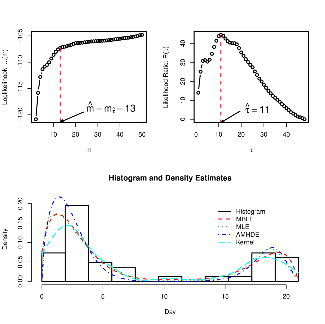
Figure 1 displays the loglikelihood , the likelihood ratio for change-points, the histogram of the grouped data and the kernel density , the MLE , the MHDE , the AMHDE , and the proposed maximum Bernstein likelihood estimate (MBLE) . From this figure we see that the proposed MBLE and the parametric MLE are similar and fit the data reasonably. The kernel density is clearly not a good estimate. The AMHDE seems to have overestimated at numbers close to 0.
6 Concluding Remarks
The proposed density estimate has obviously considerable advantages over the kernel density: (i) It is more efficient than the kernel density because it is an approximate maximum likelihood estimate; (ii) It is easier to select an optimal model degree than to select an optimal bandwidth for the kernel density; (iii) The proposed density estimate aims at which is the best approximate of for each , while the kernel density aims at , the convolution of and .
Another significance of this paper is the introduction of the acceptance-rejection argument in proving the asymptotic results where an approximate model is assumed which is new to the knowledge of the author.
Appendix A Proofs
A.1 Proof of Theorem 1
Proof.
We define as the class of functions on whose first derivatives , , exist and are continuous with the properties
| (16) |
for some , , . A polynomial of degree with “positive coefficients” is defined by Lorentz (1963) as , where , . Theorem 1 of Lorentz (1963) proved that for given integers , , and positive constants , , then there exists a constant such that for each function one can find a sequence , , of polynomials with positive coefficients of degree such that
| (17) |
where .
Under the conditions of Theorem 1, we see that , , , are finite and . So by the above result of Lorentz (1963) we have a sequence , , of polynomials with positive coefficients of degree such that
| (18) |
It is clear that
| (19) |
Since , we have, by (19),
| (20) |
Let , , then . It follows easily from (18) and (20) that (1) is true. ∎
A.2 Proof of Theorem 2
We will prove the assertion (i) only. The assertion (ii) can be proved similarly.
Proof.
The matrix of second derivatives of is
For any , as ,
Clearly, are linearly independent nonvanishing functions on [0,1]. So, with probability one, is negative definite for all and sufficiently large . By Theorem 4.2 of Redner & Walker (1984), as , converges to the maximizer of which is unique. ∎
A.3 Proof of Lemma3
Proof.
By (1) and (19) we know that under the condition of the lemma converges to at a rate of at least , i.e.,
| (21) |
and, furthermore, since ,
| (22) |
uniformly in .
Let be a sample from the uniform(0,1). By the acceptance-rejection method in simulation (Ross, 2013), for each , if , then can be treated as if it were from . Assume that the data have been rearranged so that the first observations can be treated as if they were from . By the law of iterated logarithm we have
So we have
where is an “almost complete” likelihood and
Because , we have for some constants and . By the law of iterated logarithm
| (23) | |||||
The proportion of the observations that can be treated as if they were from is
So the complete data can be viewed as a slightly contaminated sample from . ∎
A.4 Proof of Theorem 4
Proof.
The Taylor expansions of at yield that, for ,
where , a.s..
Let be a point on the boundary of , i.e., . By the law of iterated logarithm we have
and that there exists such that
Therefore we have
Since , . So there exists such that . Since , the maximum value of is attained by some with being in the interior of .
∎
A.5 Proof of Theorem 5
A.6 Proof of Theorem 6
Proof.
By (21) we have
| (24) |
where
Because we have
| (25) |
uniformly in . Assume that is a random sample from the discrete distribution with probability mass function , .
Let be a sample from the uniform(0,1). For , , let . If , then can be treated as if it were from . Assume that the data have been rearranged so that the first observations can be treated as if they were from . By the law of iterated logarithm we have
So we have
where
, , , and
It is clear that there exist and such that . By the law of iterated logarithm,
The Taylor expansions of at yield that, for ,
where , a.s..
Let be a point on the boundary of , i.e., . It follows from the law of iterated logarithm that there exists such that
Therefore
Since , . So there exists such that . Since , the maximum value of is attained by some in the interior of .
∎
A.7 Proof of Theorem 7
A.8 Proof of Theorem 8
References
- Beran (1977a) Beran, R. (1977a). Minimum Hellinger distance estimates for parametric models. Ann. Statist. 5, 445–463.
- Beran (1977b) Beran, R. (1977b). Robust location estimates. Ann. Statist. 5, 431–444.
- Bernstein (1912) Bernstein, S. N. (1912). Démonstration du théorème de Weierstrass fondée sur le calcul des probabilitiés. Comm. Soc. Math. Kharkov 13, 1–2.
- Box (1976) Box, G. E. P. (1976). Science and statistics. J. Amer. Statist. Assoc. 71, 791–799.
- Buckland (1992) Buckland, S. T. (1992). Fitting density functions with polynomials. J. Roy. Statist. Soc. Ser. C 41, 63–76.
- Csörgő & Horváth (1997) Csörgő, M. & Horváth, L. (1997). Limit Theorems in Change-Point Analysis. New York: John Wiley & Sons Inc., 1st ed.
- Dempster et al. (1977) Dempster, A. P., Laird, N. M. & Rubin, D. B. (1977). Maximum likelihood from incomplete data via the EM algorithm. J. Roy. Statist. Soc. Ser. B 39, 1–38.
- Guan (2014) Guan, Z. (2014). Efficient and Robust Density Estimation Using Bernstein Type Polynomials. ArXiv e-prints .
- Hall (1982) Hall, P. (1982). The influence of rounding errors on some nonparametric estimators of a density and its derivatives. SIAM J. Appl. Math. 42, 390–399.
- Jang & Loh (2010) Jang, W. & Loh, J. M. (2010). Density estimation for grouped data with application to line transect sampling. Ann. Appl. Stat. 4, 893–915.
- Jassim et al. (1996) Jassim, E. W., Grossman, M., Koops, W. J. & Luykx, R. A. J. (1996). Multiphasic analysis of embryonic mortality in chickens. Poultry Sci 75, 464–471.
- Jones (1993) Jones, M. C. (1993). Simple boundary correction for kernel density estimation. Statistics and Computing 3, 135–146.
- Jones et al. (1996) Jones, M. C., Marron, J. S. & Sheather, S. J. (1996). A brief survey of bandwidth selection for density estimation. Journal of the American Statistical Association 91, 401–407.
- Jones & McLachlan (1990) Jones, P. N. & McLachlan, G. J. (1990). Algorithm AS 254: Maximum likelihood estimation from grouped and truncated data with finite normal mixture models. Journal of the Royal Statistical Society. Series C (Applied Statistics) 39, 273–282.
- Kuurman et al. (2003) Kuurman, W. W., Bailey, B. A., Koops, W. J. & Grossman, M. (2003). A model for failure of a chicken embryo to survive incubation. Poultry Sci. 82, 214–222.
- Lin & He (2006) Lin, N. & He, X. (2006). Robust and efficient estimation under data grouping. Biometrika 93, 99–112.
- Lindley (1950) Lindley, D. V. (1950). Grouping corrections and maximum likelihood equations. Mathematical Proceedings of the Cambridge Philosophical Society 46, 106–110.
- Linton & Whang (2002) Linton, O. & Whang, Y.-J. (2002). Nonparametric estimation with aggregated data. Econometric Theory 18, 420–468.
- Lorentz (1963) Lorentz, G. G. (1963). The degree of approximation by polynomials with positive coefficients. Math. Ann. 151, 239–251.
- McLachlan & Jones (1988) McLachlan, G. J. & Jones, P. N. (1988). Fitting mixture models to grouped and truncated data via the EM algorithm. Biometrics 44, 571–578.
- Minoiu & Reddy (2014) Minoiu, C. & Reddy, S. (2014). Kernel density estimation on grouped data: the case of poverty assessment. The Journal of Economic Inequality 12, 163–189.
- Passow (1977) Passow, E. (1977). Polynomials with positive coefficients: uniqueness of best approximation. J. Approximation Theory 21, 352–355.
- Redner & Walker (1984) Redner, R. A. & Walker, H. F. (1984). Mixture densities, maximum likelihood and the EM algorithm. SIAM Rev. 26, 195–239.
- Rice (1984) Rice, J. (1984). Boundary modification for kernel regression. Comm. Statist. A—Theory Methods 13, 893–900.
- Rosenblatt (1956) Rosenblatt, M. (1956). Remarks on some nonparametric estimates of a density function. Ann. Math. Statist. 27, 832–837.
- Rosenblatt (1971) Rosenblatt, M. (1971). Curve estimates. Ann. Math. Statist. 42, 1815–1842.
- Ross (2013) Ross, S. M. (2013). Simulation. New York: Academic Press, 5th ed.
- Scott & Sheather (1985) Scott, D. & Sheather, S. (1985). Kernel density estimation with binned data. Communications in Statistics - Theory and Methods 14, 1353–1359.
- Sheather & Jones (1991) Sheather, S. J. & Jones, M. C. (1991). A reliable data-based bandwidth selection method for kernel density estimation. J. Roy. Statist. Soc. Ser. B 53, 683–690.
- Tallis (1967) Tallis, G. M. (1967). Approximate maximum likelihood estimates from grouped data. Technometrics 9, 599–606.
- Titterington (1983) Titterington, D. M. (1983). Kernel-based density estimation using censored, truncated or grouped data. Comm. Statist. A—Theory Methods 12, 2151–2167.
- Vitale (1975) Vitale, R. A. (1975). Bernstein polynomial approach to density function estimation. In Statistical Inference and Related Topics (Proc. Summer Res. Inst. Statist. Inference for Stochastic Processes, Indiana Univ., Bloomington, Ind., 1974, Vol. 2; dedicated to Z. W. Birnbaum). New York: Academic Press, pp. 87–99.