Best-response Algorithms for Integer Convex Quadratic Simultaneous Games

Sriram Sankaranarayanan Operations and Decision Sciences, Indian Institute of Management Ahmedabad, srirams@iima.ac.in 0000-0002-4662-3241

Abstract

We evaluate the best-response algorithm in the context of pure-integer convex quadratic games. We provide a sufficient condition that if certain interaction matrices (the product of the inverse of the positive definite matrix defining the convex quadratic terms and the matrix that connects one player’s problem to another’s) have all their singular values less than 1, then finite termination of the best-response algorithm is guaranteed regardless of the initial point. Termination is triggered through cycling among a finite number of strategies for each player. Our findings indicate that if cycling happens, a relaxed version of the Nash equilibrium can be calculated by identifying a Nash equilibrium of a smaller finite game. Conversely, we prove that if every singular value of the interaction matrices is greater than 1, the algorithm will diverge from a large family of initial points. In addition, we provide an infinite family of examples in which some of the singular values of the interaction matrices are greater than 1, cycling occurs, but any mixed-strategy with support in the strategies where cycling occurs has arbitrarily better deviations. Then, we perform computational tests of our algorithm and compare it with standard algorithms to solve such problems. We notice that our algorithm finds a Nash equilibrium correctly in every instance. Moreover, compared to a state-of-the art algorithm, our method shows similar performance in two-player games and significantly higher speed when involving three or more players.

1 Introduction

Advancements in computational power achieved over recent decades have significantly enhanced our ability to efficiently address large-scale optimization problems. Traditional optimization frameworks primarily consider an individual’s strategic choices without accommodating variations in payoffs resulting from the presence of strategic opponents or scenarios in which one player’s actions exert influence on others. The conceptualisation and formalisation of strategic interactions among players with misaligned objectives led to the introduction of game theory, notably by Morgenstern and Von Neumann (1953), Von Neumann and Morgenstern (1944). A pivotal moment in this field was John Nash’s groundbreaking theorem on the existence of equilibria, later referred to as mixed-strategy Nash equilibria, in finite games (Nash, 1950, 1951).

With the improvement in computational resources, the computation of equilibria for games has gained increasing significance and practical utility. Algorithms to obtain solutions for such games were developed in a series of papers (Ba and Pang, 2022, Bichler et al., 2023, Ravner and Snitkovsky, 2023, Feinstein and Rudloff, 2023, Carvalho et al., 2022, Adsul et al., 2021, Crönert and Minner, 2022). These equilibrium concepts find applications in identifying oligopolistic equilibria (Egging-Bratseth et al., 2020), assessing the impact of governmental policy (Langer et al., 2016), analysing infrastructure development (Devine and Siddiqui, 2023, Feijoo et al., 2018), determining pricing strategies (Luna et al., 2023), inventory decisions (Lamas and Chevalier, 2018), and even kidney exchange problems (Blom et al., 2022, Carvalho et al., 2017).

Some of these papers that work with large-scale models convexify their problem just so equilibrium identification is possible. This is driven by the computational overhead in solving games which don’t satisfy the assumptions of convexity. The literature has recently witnessed a growing interest in addressing games with structured nonconvexities, offering new perspectives on equilibrium computation. For example, there is a surge in the study of integer linear programming games, where the objectives and the constraints are linear, and some of the variables are forced to be integers (which is the nonconvexity). In this research endeavor, our focus in this paper is on a natural next step in this context, which is to consider games where each player solves a convex quadratic optimization problem with integer constraints, a specific problem category denoted as integer convex quadratic games. For such games, we explore the suitability of employing best-response algorithms. We rigorously delineate the characteristics of this game class and the associated best-response algorithm in Section 3.

The best-response algorithm.

In essence, the best-response algorithm corresponds to the dynamics where each player observes the decisions made by their counterparts in a given round and, in the subsequent round, formulates their strategy as a best response to the strategies adopted by the other players. This concept readily aligns with the notion of pure-strategy Nash equilibria, implying that, at such equilibria, no player possesses an incentive to deviate from their chosen strategy. However, when the initial state does not constitute a Nash equilibrium, players retain the flexibility to adjust their strategies in pursuit of improved payoffs. The central inquiry in this study revolves around whether this adaptive behaviour, where players respond to the strategies employed by their competitors with the assumption that their rivals will persist with the same strategies, leads to convergence to a Nash equilibrium. Notably, this assertion holds true in cases where the examined game conforms to the characteristics of a potential game (Monderer and Shapley, 1996) and the feasible sets are compact. In scenarios where such assumptions do not hold, the question of convergence becomes contingent on specific conditions. There are well-known instances of quadratic programming games with two players and one variable per player, where the best-response dynamics generate diverging iterates. We have shown the example below, as adapted from Carvalho et al. (2022, Supplementary Material, B. Divergence of SGM).

Example 1.

Consider the following simultaneous game.

\displaystyle\textbf{$\mathbf{x}$-player:}\min_{\mathbf{x}\in\mathbb{Z}}\mathbf{x}^{2}-4\mathbf{x}\mathbf{y}\qquad\qquad\qquad\qquad\textbf{$\mathbf{y}$-player:}\min_{\mathbf{y}\in\mathbb{Z}}\mathbf{y}^{2}-4\mathbf{x}\mathbf{y}

In the game given above, suppose the initial set of considered strategies for players 1 and 2 be $\{5\}$ and $\{5\}$ respectively. Setting $\mathbf{y}=5$ , player 1’s objective becomes $\mathbf{x}^{2}-20\mathbf{x}$ whose integer minimum is $\mathbf{x}=10$ . By symmetry, setting $\mathbf{x}=5$ , player 2’s optimum deviation is $\mathbf{y}=10$ . Thus the best response by each player gives a strategy pair $(10,10)$ . And from there on, the next best responses would be $(20,20)$ . Moreover, we can observe that in this procedure, the successive iterates will be $(5\times 2^{i+1},5\times 2^{i+1})$ which diverge.

The divergence here is not driven by non-existence of a Nash equilibrium as the game has a Nash equilibrium at $(0,0)$ . Further, the above is also a potential game with an exact potential function given by $\Phi(\mathbf{x},\mathbf{y})=\mathbf{x}^{2}-4\mathbf{x}\mathbf{y}+\mathbf{y}^{2}$ . While results from Monderer and Shapley (1996) hold if the feasible sets are compact, they fail when the feasible sets are the integer lattice.

Why best-response algorithm?

As a result of the above discussion, the fundamental question that arises is: why should we delve into understanding best-response dynamics in the first place? Why not exclusively rely on convexification-based methods for equilibrium identification? In many real-world scenarios, the assumption of complete information is often made for the sake of numerical tractability. However, it’s highly plausible that in practice, one player lacks access to all the parameters of another player’s optimization problem, i.e., their objectives and constraints. In such situations, a player may find themselves unable to compute a Nash equilibrium, resorting instead to crafting strategies based solely on observable actions taken by their opponents. This scenario gives rise to the concept of best-response dynamics.

Even when information is available, the adoption of best-response dynamics remains a natural choice for players with myopic perspectives, garnering significant attention within the academic discourse as well (Hopkins, 1999, Wang et al., 2021, Bayer et al., 2023, Kukushkin, 2004, Leslie et al., 2020, Morris, 2003, Voorneveld, 2000, Baudin and Laraki, 2022). Thus, understanding the convergence properties of this algorithm is of paramount importance. The negative results that we have in the paper saying that best-response dynamics are insufficient to reach an equilibrium, in practice, this corresponds to games where an external nudge is required to reach an equilibrium. This motivates our in-depth analysis of best-response dynamics within the framework of integer quadratic games.

Contributions.

We list our contributions in this paper here below.

1.

First, we present a key technical result on proximity in integer convex quadratic optimization, a result on which almost all of the fundamental results in this paper are based on. In particular, using the flatness theorem, we show that the distance between the integer minimizer and the continuous minimizer of a (strictly) convex quadratic function $f(\mathbf{x})=\frac{1}{2}\mathbf{x}^{\top}{\color[rgb]{0,0,0}\definecolor[named]{pgfstrokecolor}{rgb}{0,0,0}\pgfsys@color@gray@stroke{0}\pgfsys@color@gray@fill{0}{\mathbf{Q}}}\mathbf{x}+{\color[rgb]{0,0,0}\definecolor[named]{pgfstrokecolor}{rgb}{0,0,0}\pgfsys@color@gray@stroke{0}\pgfsys@color@gray@fill{0}{\mathbf{d}}}^{\top}\mathbf{x}$ is at most $\frac{{\color[rgb]{0,0,0}\definecolor[named]{pgfstrokecolor}{rgb}{0,0,0}\pgfsys@color@gray@stroke{0}\pgfsys@color@gray@fill{0}\phi_{n}}}{4}\sqrt{\frac{\lambda_{1}}{\lambda_{n}}}$ , where $\lambda_{1}$ and $\lambda_{n}$ are the largest and the smallest eigen values of ${\color[rgb]{0,0,0}\definecolor[named]{pgfstrokecolor}{rgb}{0,0,0}\pgfsys@color@gray@stroke{0}\pgfsys@color@gray@fill{0}{\mathbf{Q}}}$ and ${\color[rgb]{0,0,0}\definecolor[named]{pgfstrokecolor}{rgb}{0,0,0}\pgfsys@color@gray@stroke{0}\pgfsys@color@gray@fill{0}\phi_{n}}\leq n^{5/2}$ where $n$ is the dimension of $\mathbf{x}$ .
2.

For integer convex quadratic games, we provide necessary and sufficient conditions for when the best-response algorithm will terminate, irrespective of the initial iterate. The sufficient condition is that all singular values of a particular set of matrices are less than $1$ , a condition we call as the game having positively adequate objectives. The necessary condition is that at least one singular value of one of the (same set of above) matrices is less than $1$ .
3.

We show that finite termination in the context of integer convex quadratic games could occur due to cycling among finitely many strategies. In that case, we show that if $\sigma$ is a mixed-strategy Nash equilibrium (MNE) of the restricted game where each player’s strategies are restricted to those about which cycling occurs, then $\sigma$ is a $\Delta$ -MNE to the integer convex quadratic game. The paper explicitly computes the $\Delta$ that is possible.
4.

As a form of tightness to the above result, we show the following. Let $\Delta>0$ be given. There exist games where cycling occurs (without the said condition of positively adequate objectives holding), and given any MNE of the restricted game, at least one player has a deviation that improves their objective more than $\Delta$ . In other words, this shows that the proof of $\Delta$ -MNE as opposed to an actual MNE, or even a uniform bound on $\Delta$ , is not due to lack of tightness in analysis, but an inherent property of the best-response algorithm.
5.

We perform computational experiments on two classes of problems. When there are at least three players, we provide empirical evidence that our algorithm significantly outperforms the SGM algorithm (Carvalho et al., 2022). Moreover, while the theorems guarantee only a $\Delta$ -MNE with our algorithm, empirically, we always obtain an MNE. This leads us to end the paper with a conjecture that the theorem can be strengthened to state that when we have positively adequate objectives, an MNE is always retrievable.

In the appendix, we discuss the rate of convergence of the best-response algorithm to a neighbourhood of the equilibria, when our sufficient condition holds. We show that there is a linear rate of convergence, indicating that the algorithm brings the iterates close to the solution very fast. However, after reaching a neighborhood, the actual rate at which convergence occurs is not immediate from this analysis.

2 Literature Review

Finding solution strategies for games have long been of interest in the literature. As a seminal result, Lemke and Howson (1964) provided an algorithm to find Nash equilibria for bimatrix games (two-player finite games). Audet et al. (2006) improved these algorithms, and more recently, Adsul et al. (2021) provided fast algorithms to solve rank-1 bimatrix games. Also, Feinstein and Rudloff (2023) present an algorithm to solve simultaneous games with vector optimization techniques.

The term integer programming games (IPG), to the best of our knowledge, was coined in Köppe et al. (2011), marking the inception of research in this field. This unique subdomain gained prominence due to the compact representation of games with discrete strategy sets. A recent tutorial article surveys some of the algorithms in this context (Carvalho et al., 2023c).

As far as the computational complexity of IPGs go, Carvalho et al. (2022) prove that it is $\Sigma_{2}^{p}$ -hard to decide if an IPG does or does not have a PNE or an MNE. Despite the strong complexity bounds, algorithms that match the lower-bounds predicted by the complexity results have been of interest in the literature. Typically, such algorithms assume either assume linear objective functions or assume compact feasible sets or assume both. Algorithms that don’t rely on compactness of the feasible sets, typically rely on the structure of the feasible set and use a convexification approach. Carvalho et al. (2023a) identify an inner approximation-based algorithm to solve a class of problems they refer to as NASP (Nash game Among Stackelberg Players). While these problems are not directly categorised as IPGs, it is noteworthy that any bounded integer linear program can be reformulated as a continuous bilevel program. This implies the applicability of their inner-approximation algorithm to bounded integer linear programming games. As a counterpart to the inner-approximation algorithm, Carvalho et al. (2023b) proposes an outer-approximation algorithm for IPGs as well as a large class of separable games. Both these algorithms iteratively improve the approximation of the convex hull.

While both Carvalho et al. (2023b, a) suggest convexification-motivated approaches and are very fast when convexification is possible, difficulty occurs when the feasible set cannot be convexified easily. Algorithms meant to handle such settings solve finite games as a subroutine. Carvalho et al. (2022) propose the SGM algorithm, an abbreviation of Sampled Generation Method where they iteratively generate more and more feasible points and compute an MNE for the finite subset, until such an MNE is also an MNE for the entire problem. Crönert and Minner (2022) extend the algorithm into an exhaustive-SGM or eSGM algorithm, where exhaustively all MNEs of a game are enumerated, when the players’ decisions are all discrete. These algorithms, while practical and fast, require that the feasible sets are compact. Schwarze and Stein (2023) provide a branch-and-prune algorithm to identify Nash equilibria in a family of games where at least one player has an objective that is strongly convex in at least one variable.

Best-response dynamics.

Best-response dynamics have been of interest starting from the seminal paper by Monderer and Shapley (1996). The authors in this paper define a potential function, which when minimized over a compact set of feasible strategies, yields a PNE to the game. When players play the best response to the opponents in the game, they can be interpreted as descent steps in the potential function. Voorneveld (2000) extends the concept of potential function games and define best-response potential games allowing infinite paths of improvement also.

Best-response dynamics, being a very natural action for players as they only have to react to other players’ strategy in an optimal way, has been studied when we don’t have a potential function too. Hopkins (1999) provides a note comparing the best-response dynamics and other dynamics that are studied in the economics literature. Kukushkin (2004) analyses the consequences of best-response dynamics in the context of finite games with additive aggregation. Leslie et al. (2020) studies best-response dynamics in zero-sum stochastic games. Baudin and Laraki (2022) extend their work and contrast these results against fictitious plays, and also to a family of games they call identical interest games. Lei and Shanbhag (2022) consider the convergence rate of best-response dynamics in a convex stochastic game and provide bounds on equilibria based on sample size. More recently, Bayer et al. (2023) provide sufficient conditions when best-response dynamics converge to an PNE for a class of directed network games.

Within the scope of the problems addressed in this paper, the best-response optimization problem entails convex quadratic minimisation over integers, a well-explored challenge with connections to the shortest vector problem under the $\ell_{2}$ norm. This problem can be readily reduced to unconstrained convex quadratic minimisation over the integers. Conversely, any unconstrained convex quadratic minimisation over the integers can be reduced into a shortest vector problem, making both families of problems in identical complexity class. Micciancio and Voulgaris (2013) provide an optimal algorithm for the shortest vector problem, which is exponential in the number of dimensions. Given that the best-response problem is $NP$ -complete, we believe that the integer convex quadratic games does not allow for very fast algorithms in general.

3 Definitions and Algorithm descriptions

3.1 Simultaneous games

First, we define integer convex quadratic games, Nash equilibrium and the best-response algorithm.

Definition 1 (Integer Convex Quadratic Simultaneous Game (ICQS)).

An Integer Convex Quadratic Simultaneous game (ICQS) is a game of the form

	$\displaystyle\textbf{$\mathbf{x}$-player:}\min_{\mathbf{x}\in\mathbb{Z}^{n_{x}}}$	$\displaystyle:\frac{1}{2}\mathbf{x}^{\top}{\color[rgb]{0,0,0}\definecolor[named]{pgfstrokecolor}{rgb}{0,0,0}\pgfsys@color@gray@stroke{0}\pgfsys@color@gray@fill{0}{\mathbf{Q}}_{1}}\mathbf{x}+({\color[rgb]{0,0,0}\definecolor[named]{pgfstrokecolor}{rgb}{0,0,0}\pgfsys@color@gray@stroke{0}\pgfsys@color@gray@fill{0}{\mathbf{C}}_{1}}\mathbf{y}+{\color[rgb]{0,0,0}\definecolor[named]{pgfstrokecolor}{rgb}{0,0,0}\pgfsys@color@gray@stroke{0}\pgfsys@color@gray@fill{0}{\mathbf{d}}_{1}})^{\top}\mathbf{x}\qquad$
	$\displaystyle\textbf{$\mathbf{y}$-player:}\min_{\mathbf{y}\in\mathbb{Z}^{n_{y}}}$	$\displaystyle:\frac{1}{2}\mathbf{y}^{\top}{\color[rgb]{0,0,0}\definecolor[named]{pgfstrokecolor}{rgb}{0,0,0}\pgfsys@color@gray@stroke{0}\pgfsys@color@gray@fill{0}{\mathbf{Q}}_{2}}\mathbf{y}+({\color[rgb]{0,0,0}\definecolor[named]{pgfstrokecolor}{rgb}{0,0,0}\pgfsys@color@gray@stroke{0}\pgfsys@color@gray@fill{0}{\mathbf{C}}_{2}}\mathbf{x}+{\color[rgb]{0,0,0}\definecolor[named]{pgfstrokecolor}{rgb}{0,0,0}\pgfsys@color@gray@stroke{0}\pgfsys@color@gray@fill{0}{\mathbf{d}}_{2}})^{\top}\mathbf{y}$		(ICQS)

In this definition, we assume that ${\color[rgb]{0,0,0}\definecolor[named]{pgfstrokecolor}{rgb}{0,0,0}\pgfsys@color@gray@stroke{0}\pgfsys@color@gray@fill{0}{\mathbf{Q}}_{1}}$ and ${\color[rgb]{0,0,0}\definecolor[named]{pgfstrokecolor}{rgb}{0,0,0}\pgfsys@color@gray@stroke{0}\pgfsys@color@gray@fill{0}{\mathbf{Q}}_{2}}$ are symmetric positive definite matrices. Moreover, we refer to ${\color[rgb]{0,0,0}\definecolor[named]{pgfstrokecolor}{rgb}{0,0,0}\pgfsys@color@gray@stroke{0}\pgfsys@color@gray@fill{0}{\mathbf{R}}_{1}}={\color[rgb]{0,0,0}\definecolor[named]{pgfstrokecolor}{rgb}{0,0,0}\pgfsys@color@gray@stroke{0}\pgfsys@color@gray@fill{0}{\mathbf{Q}}_{1}}^{-1}{\color[rgb]{0,0,0}\definecolor[named]{pgfstrokecolor}{rgb}{0,0,0}\pgfsys@color@gray@stroke{0}\pgfsys@color@gray@fill{0}{\mathbf{C}}_{1}}$ and ${\color[rgb]{0,0,0}\definecolor[named]{pgfstrokecolor}{rgb}{0,0,0}\pgfsys@color@gray@stroke{0}\pgfsys@color@gray@fill{0}{\mathbf{R}}_{2}}={\color[rgb]{0,0,0}\definecolor[named]{pgfstrokecolor}{rgb}{0,0,0}\pgfsys@color@gray@stroke{0}\pgfsys@color@gray@fill{0}{\mathbf{Q}}_{2}}^{-1}{\color[rgb]{0,0,0}\definecolor[named]{pgfstrokecolor}{rgb}{0,0,0}\pgfsys@color@gray@stroke{0}\pgfsys@color@gray@fill{0}{\mathbf{C}}_{2}}$ as interaction matrices.

For the purposes of expositionary simplicity, we assume that there are only two players. The results in this paper can be generalized to multiple (finitely many) players. The generalized definitions with the ideas needed to extend the proofs are discussed in Appendix B. In this paper, we refer to the player choosing the $\mathbf{x}$ variables as the $\mathbf{x}$ -player, and the other one as the $\mathbf{y}$ -player. We refer to each feasible point for a player as a strategy, and a probability distribution over any finite subset of strategies as a mixed-strategy. With that, we define $\Delta$ -Mixed-strategy Nash Equilibrium (MNE).

Definition 2 ( $(\Delta_{x},\Delta_{y})$ -Nash equilibrium).

Given ICQS, a mixed-strategy pair $\sigma=(\sigma^{\mathbf{x}},\sigma^{\mathbf{y}})$ is an $(\Delta_{x},\Delta_{y})$ -mixed-strategy Nash equilibrium ( $(\Delta_{x},\Delta_{y})$ -MNE) if


$\displaystyle\mathbb{E}_{(\mathbf{x},\mathbf{y})\sim\sigma}\left[\frac{1}{2}\mathbf{x}^{\top}{\color[rgb]{0,0,0}\definecolor[named]{pgfstrokecolor}{rgb}{0,0,0}\pgfsys@color@gray@stroke{0}\pgfsys@color@gray@fill{0}{\mathbf{Q}}_{1}}\mathbf{x}+({\color[rgb]{0,0,0}\definecolor[named]{pgfstrokecolor}{rgb}{0,0,0}\pgfsys@color@gray@stroke{0}\pgfsys@color@gray@fill{0}{\mathbf{C}}_{1}}\mathbf{y}+{\color[rgb]{0,0,0}\definecolor[named]{pgfstrokecolor}{rgb}{0,0,0}\pgfsys@color@gray@stroke{0}\pgfsys@color@gray@fill{0}{\mathbf{d}}_{1}})^{\top}\mathbf{x}\right]$	$\displaystyle\leq\mathbb{E}_{\mathbf{y}\sim\sigma^{\mathbf{y}}}\left[\frac{1}{2}\mathbf{x}^{\top}{\color[rgb]{0,0,0}\definecolor[named]{pgfstrokecolor}{rgb}{0,0,0}\pgfsys@color@gray@stroke{0}\pgfsys@color@gray@fill{0}{\mathbf{Q}}_{1}}\mathbf{x}+({\color[rgb]{0,0,0}\definecolor[named]{pgfstrokecolor}{rgb}{0,0,0}\pgfsys@color@gray@stroke{0}\pgfsys@color@gray@fill{0}{\mathbf{C}}_{1}}\mathbf{y}+{\color[rgb]{0,0,0}\definecolor[named]{pgfstrokecolor}{rgb}{0,0,0}\pgfsys@color@gray@stroke{0}\pgfsys@color@gray@fill{0}{\mathbf{d}}_{1}})^{\top}\mathbf{x}\right]+\Delta_{x}$	$\displaystyle\forall\mathbf{x}\in\mathbb{Z}^{n_{x}}$
$\displaystyle\mathbb{E}_{(\mathbf{x},\mathbf{y})\sim\sigma}\left[\frac{1}{2}\mathbf{y}^{\top}{\color[rgb]{0,0,0}\definecolor[named]{pgfstrokecolor}{rgb}{0,0,0}\pgfsys@color@gray@stroke{0}\pgfsys@color@gray@fill{0}{\mathbf{Q}}_{2}}\mathbf{y}+({\color[rgb]{0,0,0}\definecolor[named]{pgfstrokecolor}{rgb}{0,0,0}\pgfsys@color@gray@stroke{0}\pgfsys@color@gray@fill{0}{\mathbf{C}}_{2}}\mathbf{x}+{\color[rgb]{0,0,0}\definecolor[named]{pgfstrokecolor}{rgb}{0,0,0}\pgfsys@color@gray@stroke{0}\pgfsys@color@gray@fill{0}{\mathbf{d}}_{1}})^{\top}\mathbf{y}\right]$	$\displaystyle\leq\mathbb{E}_{\mathbf{x}\sim\sigma^{\mathbf{x}}}\left[\frac{1}{2}\mathbf{y}^{\top}{\color[rgb]{0,0,0}\definecolor[named]{pgfstrokecolor}{rgb}{0,0,0}\pgfsys@color@gray@stroke{0}\pgfsys@color@gray@fill{0}{\mathbf{Q}}_{2}}\mathbf{y}+({\color[rgb]{0,0,0}\definecolor[named]{pgfstrokecolor}{rgb}{0,0,0}\pgfsys@color@gray@stroke{0}\pgfsys@color@gray@fill{0}{\mathbf{C}}_{2}}\mathbf{x}+{\color[rgb]{0,0,0}\definecolor[named]{pgfstrokecolor}{rgb}{0,0,0}\pgfsys@color@gray@stroke{0}\pgfsys@color@gray@fill{0}{\mathbf{d}}_{2}})^{\top}\mathbf{y}\right]+\Delta_{y}$	$\displaystyle\forall\mathbf{y}\in\mathbb{Z}^{n_{y}}$

Further, the finite subset of $\mathbb{Z}^{n_{x}}$ and $\mathbb{Z}^{n_{y}}$ to which $\sigma^{\mathbf{x}}$ and $\sigma^{\mathbf{y}}$ assign non-zero probability are called the $\mathbf{x}$ -player’s and $\mathbf{y}$ -player’s supports of the $(\Delta_{x},\Delta_{y})$ -MNE respectively. If $\Delta_{x}=\Delta_{y}=0$ holds, then we call it just an MNE or a PNE.

We note the subtle difference between $\varepsilon$ -MNE that is popular in literature as opposed to the $\Delta$ -MNE we define above. Typically, algorithms claim to find an $\varepsilon$ -MNE, if such solution is possible for any given $\varepsilon>0$ , i.e., any allowable positive error. In contrast, our paper only guarantees solutions for a fixed value of the error term that we denote by $\Delta$ . Besides this subtle difference, the definitions are interchangable.

3.2 The best-response algorithm

Definition 3 (Best Response).

Given a game ICQS, we define the best response of the $\mathbf{x}$ -player, given $\mathbf{y}$ as ${\color[rgb]{0,0,0}\definecolor[named]{pgfstrokecolor}{rgb}{0,0,0}\pgfsys@color@gray@stroke{0}\pgfsys@color@gray@fill{0}{\color[rgb]{0,0,0}\definecolor[named]{pgfstrokecolor}{rgb}{0,0,0}\pgfsys@color@gray@stroke{0}\pgfsys@color@gray@fill{0}\mathcal{B}}_{1}\left(\mathbf{y}\right)}\in\arg\min_{x}\left\{\frac{1}{2}\mathbf{x}^{\top}{\color[rgb]{0,0,0}\definecolor[named]{pgfstrokecolor}{rgb}{0,0,0}\pgfsys@color@gray@stroke{0}\pgfsys@color@gray@fill{0}{\mathbf{Q}}_{1}}\mathbf{x}+\left({\color[rgb]{0,0,0}\definecolor[named]{pgfstrokecolor}{rgb}{0,0,0}\pgfsys@color@gray@stroke{0}\pgfsys@color@gray@fill{0}{\mathbf{C}}_{1}}\mathbf{y}+{\color[rgb]{0,0,0}\definecolor[named]{pgfstrokecolor}{rgb}{0,0,0}\pgfsys@color@gray@stroke{0}\pgfsys@color@gray@fill{0}{\mathbf{d}}_{1}}\right)^{\top}\mathbf{x}\mid\mathbf{x}\in\mathbb{Z}^{n_{x}}\right\}$ and the best response of the $\mathbf{y}$ -player given $\mathbf{x}$ as ${\color[rgb]{0,0,0}\definecolor[named]{pgfstrokecolor}{rgb}{0,0,0}\pgfsys@color@gray@stroke{0}\pgfsys@color@gray@fill{0}{\color[rgb]{0,0,0}\definecolor[named]{pgfstrokecolor}{rgb}{0,0,0}\pgfsys@color@gray@stroke{0}\pgfsys@color@gray@fill{0}\mathcal{B}}_{2}\left(\mathbf{x}\right)}\in\arg\min_{y}\left\{\frac{1}{2}\mathbf{y}^{\top}{\color[rgb]{0,0,0}\definecolor[named]{pgfstrokecolor}{rgb}{0,0,0}\pgfsys@color@gray@stroke{0}\pgfsys@color@gray@fill{0}{\mathbf{Q}}_{2}}\mathbf{y}+\left({\color[rgb]{0,0,0}\definecolor[named]{pgfstrokecolor}{rgb}{0,0,0}\pgfsys@color@gray@stroke{0}\pgfsys@color@gray@fill{0}{\mathbf{C}}_{2}}\mathbf{x}+{\color[rgb]{0,0,0}\definecolor[named]{pgfstrokecolor}{rgb}{0,0,0}\pgfsys@color@gray@stroke{0}\pgfsys@color@gray@fill{0}{\mathbf{d}}_{2}}\right)^{\top}\mathbf{y}\mid\mathbf{y}\in\mathbb{Z}^{n_{y}}\right\}$ .

We note that ${\color[rgb]{0,0,0}\definecolor[named]{pgfstrokecolor}{rgb}{0,0,0}\pgfsys@color@gray@stroke{0}\pgfsys@color@gray@fill{0}{\color[rgb]{0,0,0}\definecolor[named]{pgfstrokecolor}{rgb}{0,0,0}\pgfsys@color@gray@stroke{0}\pgfsys@color@gray@fill{0}\mathcal{B}}_{1}\left(\mathbf{y}\right)}$ and ${\color[rgb]{0,0,0}\definecolor[named]{pgfstrokecolor}{rgb}{0,0,0}\pgfsys@color@gray@stroke{0}\pgfsys@color@gray@fill{0}{\color[rgb]{0,0,0}\definecolor[named]{pgfstrokecolor}{rgb}{0,0,0}\pgfsys@color@gray@stroke{0}\pgfsys@color@gray@fill{0}\mathcal{B}}_{2}\left(\mathbf{x}\right)}$ need not be singleton sets. If they are not singleton, for the purposes of the best-response algorithm, any arbitrary element from these sets can be chosen.

The notion of best response immediately presents the idea of a best-response algorithm which is formally presented in Algorithm 1.

Algorithm 1 is possibly one of the simplest algorithms that could be considered for finding Nash equilibria for simultaneous games. We begin with input “guesses” for each player’s strategy – $\widehat{\mathbf{x}}^{0}$ and $\widehat{\mathbf{y}}^{0}$ . In 5 we solve integer convex quadratic programs to identify the best response to the previous strategy of the other player. We repeat this until a previously-observed iterate is observed again.

Algorithm 1 The Best-Response Algorithm

1:ICQS instance

({\color[rgb]{0,0,0}\definecolor[named]{pgfstrokecolor}{rgb}{0,0,0}\pgfsys@color@gray@stroke{0}\pgfsys@color@gray@fill{0}{\mathbf{Q}}_{1}},{\color[rgb]{0,0,0}\definecolor[named]{pgfstrokecolor}{rgb}{0,0,0}\pgfsys@color@gray@stroke{0}\pgfsys@color@gray@fill{0}{\mathbf{Q}}_{2}},{\color[rgb]{0,0,0}\definecolor[named]{pgfstrokecolor}{rgb}{0,0,0}\pgfsys@color@gray@stroke{0}\pgfsys@color@gray@fill{0}{\mathbf{C}}_{1}},{\color[rgb]{0,0,0}\definecolor[named]{pgfstrokecolor}{rgb}{0,0,0}\pgfsys@color@gray@stroke{0}\pgfsys@color@gray@fill{0}{\mathbf{C}}_{2}},{\color[rgb]{0,0,0}\definecolor[named]{pgfstrokecolor}{rgb}{0,0,0}\pgfsys@color@gray@stroke{0}\pgfsys@color@gray@fill{0}{\mathbf{d}}_{1}},{\color[rgb]{0,0,0}\definecolor[named]{pgfstrokecolor}{rgb}{0,0,0}\pgfsys@color@gray@stroke{0}\pgfsys@color@gray@fill{0}{\mathbf{d}}_{2}})

and

(\widehat{\mathbf{x}}^{0},\widehat{\mathbf{y}}^{0})\in\mathbb{Z}^{n_{x}+n_{y}}

2:Two finite sets

S_{x}

and

S_{y}

such that for all

\mathbf{x}\in S_{x}

{\color[rgb]{0,0,0}\definecolor[named]{pgfstrokecolor}{rgb}{0,0,0}\pgfsys@color@gray@stroke{0}\pgfsys@color@gray@fill{0}{\color[rgb]{0,0,0}\definecolor[named]{pgfstrokecolor}{rgb}{0,0,0}\pgfsys@color@gray@stroke{0}\pgfsys@color@gray@fill{0}\mathcal{B}}_{2}\left(\mathbf{x}\right)}\in S_{y}

and for all

\mathbf{y}\in S_{y}

{\color[rgb]{0,0,0}\definecolor[named]{pgfstrokecolor}{rgb}{0,0,0}\pgfsys@color@gray@stroke{0}\pgfsys@color@gray@fill{0}{\color[rgb]{0,0,0}\definecolor[named]{pgfstrokecolor}{rgb}{0,0,0}\pgfsys@color@gray@stroke{0}\pgfsys@color@gray@fill{0}\mathcal{B}}_{1}\left(\mathbf{y}\right)}\in S_{x}

i\leftarrow 1

4:loop

\widehat{\mathbf{x}}^{i}\leftarrow{\color[rgb]{0,0,0}\definecolor[named]{pgfstrokecolor}{rgb}{0,0,0}\pgfsys@color@gray@stroke{0}\pgfsys@color@gray@fill{0}{\color[rgb]{0,0,0}\definecolor[named]{pgfstrokecolor}{rgb}{0,0,0}\pgfsys@color@gray@stroke{0}\pgfsys@color@gray@fill{0}\mathcal{B}}_{1}\left(\widehat{\mathbf{y}}^{i-1}\right)}

\widehat{\mathbf{y}}^{i}\leftarrow{\color[rgb]{0,0,0}\definecolor[named]{pgfstrokecolor}{rgb}{0,0,0}\pgfsys@color@gray@stroke{0}\pgfsys@color@gray@fill{0}{\color[rgb]{0,0,0}\definecolor[named]{pgfstrokecolor}{rgb}{0,0,0}\pgfsys@color@gray@stroke{0}\pgfsys@color@gray@fill{0}\mathcal{B}}_{2}\left(\widehat{\mathbf{x}}^{i-1}\right)}

6: if

\widehat{\mathbf{x}}^{i}=\widehat{\mathbf{x}}^{k}

and

\widehat{\mathbf{y}}^{i}=\widehat{\mathbf{y}}^{k}

for some

k<i

then

7: return

S_{x}=\{\widehat{\mathbf{x}}^{k},\widehat{\mathbf{x}}^{k+1},\dots,\widehat{\mathbf{x}}^{i}\}

S_{y}=\{\widehat{\mathbf{y}}^{k},\widehat{\mathbf{y}}^{k+1},\dots,\widehat{\mathbf{y}}^{i}\}

8: end if

i\leftarrow i+1

10:end loop

Observe that it is not possible for the iterates to converge to a point but not attain the limit. This is beacuse, each iterate is a feasible point in the integer lattice, and they can’t get arbitrarily closer without coinciding. Thus the only two outcomes are (i) the algorithm cycling among finitely many strategies (and hence terminating) or (ii) diverging (non-terminating). Cycle could be of length $1$ , in which case, the repeated strategy is a pure-strategy Nash equilibrium. Alternatively, it could also be of some finite length.

3.3 Adequate objectives

Before we state the main results, we define positively and negatively adequate objectives below. A game having (positively or negatively) adequate objectives is a combined property of the objectives of both the players. More importantly, this can be checked only by inspecting the singular values of a the interaction matrices ${\color[rgb]{0,0,0}\definecolor[named]{pgfstrokecolor}{rgb}{0,0,0}\pgfsys@color@gray@stroke{0}\pgfsys@color@gray@fill{0}{\mathbf{R}}_{1}}$ and ${\color[rgb]{0,0,0}\definecolor[named]{pgfstrokecolor}{rgb}{0,0,0}\pgfsys@color@gray@stroke{0}\pgfsys@color@gray@fill{0}{\mathbf{R}}_{2}}$ . There are efficient routines to do a singular value decomposition of any matrix $\mathbf{A}=\mathbf{U}\mathbf{\Sigma}\mathbf{V}$ , where $\mathbf{U},\mathbf{V}$ are unitary matrices and $\mathbf{\Sigma}$ is a non-negative codiagonal matrix. The diagonal elements of $\mathbf{\Sigma}$ are the singular values of $A$ .

Definition 4.

ICQS is said to have positively adequate objectives if every singular value of the interaction matrices ${\color[rgb]{0,0,0}\definecolor[named]{pgfstrokecolor}{rgb}{0,0,0}\pgfsys@color@gray@stroke{0}\pgfsys@color@gray@fill{0}{\mathbf{R}}_{1}}$ and ${\color[rgb]{0,0,0}\definecolor[named]{pgfstrokecolor}{rgb}{0,0,0}\pgfsys@color@gray@stroke{0}\pgfsys@color@gray@fill{0}{\mathbf{R}}_{2}}$ is strictly less than $1.$

Definition 5.

ICQS is said to have negatively adequate objectives if every singular value of the interaction matrices ${\color[rgb]{0,0,0}\definecolor[named]{pgfstrokecolor}{rgb}{0,0,0}\pgfsys@color@gray@stroke{0}\pgfsys@color@gray@fill{0}{\mathbf{R}}_{1}}$ and ${\color[rgb]{0,0,0}\definecolor[named]{pgfstrokecolor}{rgb}{0,0,0}\pgfsys@color@gray@stroke{0}\pgfsys@color@gray@fill{0}{\mathbf{R}}_{2}}$ is strictly greater than $1.$

When we have positively adequate objectives, we assume that the largest singular value is $1-\rho$ for some $\rho>0$ and when we have negatively adequate objectives, we assume that the smallest singular value is $1+\rho$ for some $\rho>0$ .

4 Main Results

We state the organization of results in this paper first. First we prove a technical result we call proximity theorem (Theorem 3) that provides a bound for the maximum distance between a continuous minimizer and an integer minimizer of a convex quadratic function, a bound that is insensitive to the linear terms of the convex quadratic function. Using this result and the assumption of positively adequate objectives, we show that Algorithm 1 terminates finitely (Theorem 1). Then, we show a negative result, that if the game has negatively adequate objectives, there always exists points from where Algorithm 1 generates divergent iterates (Theorem 2). Together, Theorems 2 and 1 provide necessary and sufficient conditions for finite termination of Algorithm 1.

Following the results on finite termination, we consider the part where we solve a finite game restricted to the iterates about which Algorithm 1 cycled to obtain an MNE. First, we show that in general, such an MNE to the restricted finite game could be arbitrarily bad for the original instance of ICQS (Theorem 4). Then, we show that, the maximum profitable deviation any player in ICQS could obtain, given an MNE for the finitely restricted game, is bounded by the maximum distance between any pair of iterates generated (Theorem 5). Next, we show that under our assumption of positively adequate objectives, the maximum distance between any two iterates about which cycling happens is indeed bounded (Theorem 6). Tying these results together, we have Corollary 1, which says that under the assumption of positively adequate objectives, Algorithm 1 can be used to obtain $\Delta$ -MNE. Finally, from the computational experience, we state a conjecture that in case of positively adequate objectives, the value $\Delta$ can be indeed chosen as zero.

For enhanced readability, we show the implications between the theorems in the manuscript in Figure 1.

Refer to caption — Figure 1: Implications among Theorems

4.1 Necessary and sufficient conditions for finite termination

Theorem 1.

If the game ICQS has positively adequate objectives, then Algorithm 1 terminates finitely, irrespective of the initial points $\widehat{\mathbf{x}}^{0},\widehat{\mathbf{y}}^{0}$ .

Theorem 2.

If the game ICQS has negatively adequate objectives, then Algorithm 1 generates divergent iterates for all but finitely many feasible initial points $\widehat{\mathbf{x}}^{0},\widehat{\mathbf{y}}^{0}$ .

Theorems 2 and 1 can be interpreted respectively as necessary and sufficient conditions for Algorithm 1 to terminate finitely. However, proving these requires an intermediate result on proximity of integer minimizers of convex quadratic functions to the corresponding continuous minimizers. In that respect, we first define proximity bound, and then we prove that the bound is finite for any given positive definite matrix ${\color[rgb]{0,0,0}\definecolor[named]{pgfstrokecolor}{rgb}{0,0,0}\pgfsys@color@gray@stroke{0}\pgfsys@color@gray@fill{0}{\mathbf{Q}}}$ .

4.2 Proximity in integer convex quadratic programs

First, we define proximity, which bounds the maximum distance between the continuous minimum and the integer minimum of a convex quadratic function. The most famous of such results are the results in the context of linear programs provided in Cook et al. (1986), and recently improved by Paat et al. (2020), Celaya et al. (2022). Some proximity results for convex quadratic programs (Granot and Skorin-Kapov, 1990) and a subfamily of general convex programs (Moriguchi et al., 2011) are available in the literature extending the results for integer linear programs. We provide a version of proximity result for convex quadratic programs in this paper. While the results are not in full generality in line with the proximity literature in the context of integer linear programs, the version we provide here is sufficient to prove the fundamental results of the paper.

Definition 6.

Let ${\color[rgb]{0,0,0}\definecolor[named]{pgfstrokecolor}{rgb}{0,0,0}\pgfsys@color@gray@stroke{0}\pgfsys@color@gray@fill{0}{\mathbf{Q}}}$ be a given positive definite matrix. The proximity bound of ${\color[rgb]{0,0,0}\definecolor[named]{pgfstrokecolor}{rgb}{0,0,0}\pgfsys@color@gray@stroke{0}\pgfsys@color@gray@fill{0}{\mathbf{Q}}}$ with respect to the $\ell_{p}$ vector norm is denoted by ${\color[rgb]{0,0,0}\definecolor[named]{pgfstrokecolor}{rgb}{0,0,0}\pgfsys@color@gray@stroke{0}\pgfsys@color@gray@fill{0}{\color[rgb]{0,0,0}\definecolor[named]{pgfstrokecolor}{rgb}{0,0,0}\pgfsys@color@gray@stroke{0}\pgfsys@color@gray@fill{0}\pi}_{p}\left({\color[rgb]{0,0,0}\definecolor[named]{pgfstrokecolor}{rgb}{0,0,0}\pgfsys@color@gray@stroke{0}\pgfsys@color@gray@fill{0}{\mathbf{Q}}}\right)}$ and is the optimal objective value of the problem


$\displaystyle\max_{{\color[rgb]{0,0,0}\definecolor[named]{pgfstrokecolor}{rgb}{0,0,0}\pgfsys@color@gray@stroke{0}\pgfsys@color@gray@fill{0}{\mathbf{d}}}\in\mathbb{R}^{n}}\max_{\begin{subarray}{c}\mathbf{u}\in\mathbb{R}^{n}\\ \mathbf{v}\in\mathbb{Z}^{n}\end{subarray}}$	$\displaystyle:\left\\|\mathbf{u}-\mathbf{v}\right\\|_{p}$	s.t.	(2a)
$\displaystyle\mathbf{u}$	$\displaystyle\in\arg\min\left\{\frac{1}{2}\mathbf{x}^{\top}{\color[rgb]{0,0,0}\definecolor[named]{pgfstrokecolor}{rgb}{0,0,0}\pgfsys@color@gray@stroke{0}\pgfsys@color@gray@fill{0}{\mathbf{Q}}}\mathbf{x}+{\color[rgb]{0,0,0}\definecolor[named]{pgfstrokecolor}{rgb}{0,0,0}\pgfsys@color@gray@stroke{0}\pgfsys@color@gray@fill{0}{\mathbf{d}}}^{\top}\mathbf{x}:\mathbf{x}\in\mathbb{R}^{n}\right\}$		(2b)
$\displaystyle\mathbf{v}$	$\displaystyle\in\arg\min\left\{\frac{1}{2}\mathbf{x}^{\top}{\color[rgb]{0,0,0}\definecolor[named]{pgfstrokecolor}{rgb}{0,0,0}\pgfsys@color@gray@stroke{0}\pgfsys@color@gray@fill{0}{\mathbf{Q}}}\mathbf{x}+{\color[rgb]{0,0,0}\definecolor[named]{pgfstrokecolor}{rgb}{0,0,0}\pgfsys@color@gray@stroke{0}\pgfsys@color@gray@fill{0}{\mathbf{d}}}^{\top}\mathbf{x}:\mathbf{x}\in\mathbb{Z}^{n}\right\}$		(2c)

In this paper, we use $\ell_{2}$ norm predominantly, so when referring to ${\color[rgb]{0,0,0}\definecolor[named]{pgfstrokecolor}{rgb}{0,0,0}\pgfsys@color@gray@stroke{0}\pgfsys@color@gray@fill{0}{\color[rgb]{0,0,0}\definecolor[named]{pgfstrokecolor}{rgb}{0,0,0}\pgfsys@color@gray@stroke{0}\pgfsys@color@gray@fill{0}\pi}_{2}\left({\color[rgb]{0,0,0}\definecolor[named]{pgfstrokecolor}{rgb}{0,0,0}\pgfsys@color@gray@stroke{0}\pgfsys@color@gray@fill{0}{\mathbf{Q}}}\right)}$ we write ${\color[rgb]{0,0,0}\definecolor[named]{pgfstrokecolor}{rgb}{0,0,0}\pgfsys@color@gray@stroke{0}\pgfsys@color@gray@fill{0}{\color[rgb]{0,0,0}\definecolor[named]{pgfstrokecolor}{rgb}{0,0,0}\pgfsys@color@gray@stroke{0}\pgfsys@color@gray@fill{0}\pi}\left({\color[rgb]{0,0,0}\definecolor[named]{pgfstrokecolor}{rgb}{0,0,0}\pgfsys@color@gray@stroke{0}\pgfsys@color@gray@fill{0}{\mathbf{Q}}}\right)}$ .

In Definition 6, we consider a quadratic function whose quadratic terms (defined by ${\color[rgb]{0,0,0}\definecolor[named]{pgfstrokecolor}{rgb}{0,0,0}\pgfsys@color@gray@stroke{0}\pgfsys@color@gray@fill{0}{\mathbf{Q}}}$ ) are fixed, but the linear terms (defined by ${\color[rgb]{0,0,0}\definecolor[named]{pgfstrokecolor}{rgb}{0,0,0}\pgfsys@color@gray@stroke{0}\pgfsys@color@gray@fill{0}{\mathbf{d}}}$ ) are allowed to vary. We want to find the linear term ${\color[rgb]{0,0,0}\definecolor[named]{pgfstrokecolor}{rgb}{0,0,0}\pgfsys@color@gray@stroke{0}\pgfsys@color@gray@fill{0}{\mathbf{d}}}$ such that the distance between the continuous minimizer $\mathbf{u}$ and the integer minimizer $\mathbf{v}$ is maximized. Moreover, the inner $\max$ ensures, should there be multiple integer minimizers, a minimizer which is farthest from the (unique) continuous minimizer could be chosen.

Apriori, it is not clear if ${\color[rgb]{0,0,0}\definecolor[named]{pgfstrokecolor}{rgb}{0,0,0}\pgfsys@color@gray@stroke{0}\pgfsys@color@gray@fill{0}{\color[rgb]{0,0,0}\definecolor[named]{pgfstrokecolor}{rgb}{0,0,0}\pgfsys@color@gray@stroke{0}\pgfsys@color@gray@fill{0}\pi}\left({\color[rgb]{0,0,0}\definecolor[named]{pgfstrokecolor}{rgb}{0,0,0}\pgfsys@color@gray@stroke{0}\pgfsys@color@gray@fill{0}{\mathbf{Q}}}\right)}$ is finite for a given ${\color[rgb]{0,0,0}\definecolor[named]{pgfstrokecolor}{rgb}{0,0,0}\pgfsys@color@gray@stroke{0}\pgfsys@color@gray@fill{0}{\mathbf{Q}}}$ . It is not clear if for a given ${\color[rgb]{0,0,0}\definecolor[named]{pgfstrokecolor}{rgb}{0,0,0}\pgfsys@color@gray@stroke{0}\pgfsys@color@gray@fill{0}{\mathbf{Q}}}$ there is a sequence of ${\color[rgb]{0,0,0}\definecolor[named]{pgfstrokecolor}{rgb}{0,0,0}\pgfsys@color@gray@stroke{0}\pgfsys@color@gray@fill{0}{\mathbf{d}}}^{1},{\color[rgb]{0,0,0}\definecolor[named]{pgfstrokecolor}{rgb}{0,0,0}\pgfsys@color@gray@stroke{0}\pgfsys@color@gray@fill{0}{\mathbf{d}}}^{2},\dots$ and corresponding continuous minimizers $\mathbf{u}^{1},\mathbf{u}^{2},\dots$ and integer minimizers, $\mathbf{v}^{1},\mathbf{v}^{2},\dots$ of the quadratic such that $\left\|\mathbf{u}^{i}-\mathbf{v}^{i}\right\|\to\infty$ . However, we show that this is not the case in the following result.

Theorem 3 (Proximity Theorem).

Given a positive definite matrix ${\color[rgb]{0,0,0}\definecolor[named]{pgfstrokecolor}{rgb}{0,0,0}\pgfsys@color@gray@stroke{0}\pgfsys@color@gray@fill{0}{\mathbf{Q}}}$ of dimension $n\times n$ ,

(i)

${\color[rgb]{0,0,0}\definecolor[named]{pgfstrokecolor}{rgb}{0,0,0}\pgfsys@color@gray@stroke{0}\pgfsys@color@gray@fill{0}{\color[rgb]{0,0,0}\definecolor[named]{pgfstrokecolor}{rgb}{0,0,0}\pgfsys@color@gray@stroke{0}\pgfsys@color@gray@fill{0}\pi}\left({\color[rgb]{0,0,0}\definecolor[named]{pgfstrokecolor}{rgb}{0,0,0}\pgfsys@color@gray@stroke{0}\pgfsys@color@gray@fill{0}{\mathbf{Q}}}\right)}\leq\frac{{\color[rgb]{0,0,0}\definecolor[named]{pgfstrokecolor}{rgb}{0,0,0}\pgfsys@color@gray@stroke{0}\pgfsys@color@gray@fill{0}\phi_{n}}}{4}\sqrt{\frac{\lambda_{1}}{\lambda_{n}}}$ .
(ii)

The maximum difference between the optimal objective values when optimizing over $\mathbb{R}^{n}$ versus optimizing over $\mathbb{Z}^{n}$ is $\frac{\lambda_{1}{\color[rgb]{0,0,0}\definecolor[named]{pgfstrokecolor}{rgb}{0,0,0}\pgfsys@color@gray@stroke{0}\pgfsys@color@gray@fill{0}\phi_{n}}^{2}}{32}$ .

where $\lambda_{1}$ and $\lambda_{n}$ are the largest and the smallest singular values of ${\color[rgb]{0,0,0}\definecolor[named]{pgfstrokecolor}{rgb}{0,0,0}\pgfsys@color@gray@stroke{0}\pgfsys@color@gray@fill{0}{\mathbf{Q}}}$ and ${\color[rgb]{0,0,0}\definecolor[named]{pgfstrokecolor}{rgb}{0,0,0}\pgfsys@color@gray@stroke{0}\pgfsys@color@gray@fill{0}\phi_{n}}$ is a constant dependent only on the dimension $n$ .

First we note that since ${\color[rgb]{0,0,0}\definecolor[named]{pgfstrokecolor}{rgb}{0,0,0}\pgfsys@color@gray@stroke{0}\pgfsys@color@gray@fill{0}{\mathbf{Q}}}$ is a real symmetric matrix, the absolute value of its eigen values are its singular values. Moreover, since ${\color[rgb]{0,0,0}\definecolor[named]{pgfstrokecolor}{rgb}{0,0,0}\pgfsys@color@gray@stroke{0}\pgfsys@color@gray@fill{0}{\mathbf{Q}}}$ is positive definite, all its eigen values are positive real numbers. So, its eigen values are its singular values. Thus $\lambda_{1}$ and $\lambda_{n}$ in Theorem 3 can also be interpreted as the largest and the smallest eigen values of ${\color[rgb]{0,0,0}\definecolor[named]{pgfstrokecolor}{rgb}{0,0,0}\pgfsys@color@gray@stroke{0}\pgfsys@color@gray@fill{0}{\mathbf{Q}}}$ .

To prove Theorem 3, we use a fundamental result in convex analysis named the flatness theorem. We refer the readers to Barvinok (2002, Pg. 317, Theorem 8.3) for a complete and formal proof of the flatness theorem. The theorem states that if a convex set $C\subseteq\mathbb{R}^{n}$ has no integer points in its interior, then there exists an (integer) direction $\mathbf{z}\in\mathbb{Z}^{n}\setminus\{0\}$ along which the convex set $C$ is flat. i.e., there exists $\mathbf{z}\in\mathbb{Z}^{n}\setminus\{0\}$ such that $\max\{\mathbf{z}^{\top}\mathbf{x}:\mathbf{x}\in C\}-\min\{\mathbf{z}^{\top}\mathbf{x}:\mathbf{x}\in C\}\leq{\color[rgb]{0,0,0}\definecolor[named]{pgfstrokecolor}{rgb}{0,0,0}\pgfsys@color@gray@stroke{0}\pgfsys@color@gray@fill{0}\phi_{n}}$ , a finite number dependent only on the dimension $n$ of the space in which $C$ lies. While the theorem is generally stated for any lattice, in this paper we are only interested in $\mathbb{Z}^{n}$ lattice. For $\mathbb{Z}^{n}$ , it is known that ${\color[rgb]{0,0,0}\definecolor[named]{pgfstrokecolor}{rgb}{0,0,0}\pgfsys@color@gray@stroke{0}\pgfsys@color@gray@fill{0}\phi_{n}}\leq n^{5/2}$ , although stronger ( $\mathcal{O}(n)$ ) bounds are conjectured (Celaya et al., 2022, Rudelson, 2000). We state all our results in terms of ${\color[rgb]{0,0,0}\definecolor[named]{pgfstrokecolor}{rgb}{0,0,0}\pgfsys@color@gray@stroke{0}\pgfsys@color@gray@fill{0}\phi_{n}}$ , so if stronger bounds are found for ${\color[rgb]{0,0,0}\definecolor[named]{pgfstrokecolor}{rgb}{0,0,0}\pgfsys@color@gray@stroke{0}\pgfsys@color@gray@fill{0}\phi_{n}}$ , they are directly applicable here.

Proof of Theorem 3..

Consider a strictly convex quadratic function $\frac{1}{2}\mathbf{x}^{\top}Q\mathbf{x}+{\color[rgb]{0,0,0}\definecolor[named]{pgfstrokecolor}{rgb}{0,0,0}\pgfsys@color@gray@stroke{0}\pgfsys@color@gray@fill{0}{\mathbf{d}}}^{\top}\mathbf{x}$ . For the choice $\mathbf{u}=-{\color[rgb]{0,0,0}\definecolor[named]{pgfstrokecolor}{rgb}{0,0,0}\pgfsys@color@gray@stroke{0}\pgfsys@color@gray@fill{0}{\mathbf{Q}}}^{-1}{\color[rgb]{0,0,0}\definecolor[named]{pgfstrokecolor}{rgb}{0,0,0}\pgfsys@color@gray@stroke{0}\pgfsys@color@gray@fill{0}{\mathbf{d}}}$ (equivalently ${\color[rgb]{0,0,0}\definecolor[named]{pgfstrokecolor}{rgb}{0,0,0}\pgfsys@color@gray@stroke{0}\pgfsys@color@gray@fill{0}{\mathbf{d}}}=-{\color[rgb]{0,0,0}\definecolor[named]{pgfstrokecolor}{rgb}{0,0,0}\pgfsys@color@gray@stroke{0}\pgfsys@color@gray@fill{0}{\mathbf{Q}}}\mathbf{u}$ ), we can rewrite the function as $\frac{1}{2}\mathbf{x}^{\top}Q\mathbf{x}-\mathbf{u}^{\top}{\color[rgb]{0,0,0}\definecolor[named]{pgfstrokecolor}{rgb}{0,0,0}\pgfsys@color@gray@stroke{0}\pgfsys@color@gray@fill{0}{\mathbf{Q}}}\mathbf{x}$ . Neither the continuous minimizer nor the integer minimizer is sensitive to addition of constants to the function. Thus the continuous and the integer minimizers of the above function are same as that of $\frac{1}{2}\mathbf{x}^{\top}Q\mathbf{x}-\mathbf{u}^{\top}{\color[rgb]{0,0,0}\definecolor[named]{pgfstrokecolor}{rgb}{0,0,0}\pgfsys@color@gray@stroke{0}\pgfsys@color@gray@fill{0}{\mathbf{Q}}}\mathbf{x}+\frac{1}{2}\mathbf{u}^{\top}\mathbf{u}$ . But this expression equals $\frac{1}{2}(\mathbf{x}-\mathbf{u})^{\top}{\color[rgb]{0,0,0}\definecolor[named]{pgfstrokecolor}{rgb}{0,0,0}\pgfsys@color@gray@stroke{0}\pgfsys@color@gray@fill{0}{\mathbf{Q}}}(\mathbf{x}-\mathbf{u})$ . We have written a general strictly convex quadratic function in the above form. Thus, it is sufficient to consider quadratic functions in this form. Define $f_{u}(\mathbf{x}):=\frac{1}{2}(\mathbf{x}-\mathbf{u})^{\top}{\color[rgb]{0,0,0}\definecolor[named]{pgfstrokecolor}{rgb}{0,0,0}\pgfsys@color@gray@stroke{0}\pgfsys@color@gray@fill{0}{\mathbf{Q}}}(\mathbf{x}-\mathbf{u})$ . A useful property when considering this form is that $\mathbf{u}$ is the continuous minimizer here, and we don’t need to explicitly write ${\color[rgb]{0,0,0}\definecolor[named]{pgfstrokecolor}{rgb}{0,0,0}\pgfsys@color@gray@stroke{0}\pgfsys@color@gray@fill{0}{\mathbf{d}}}$ as a part of the function. The corresponding value of ${\color[rgb]{0,0,0}\definecolor[named]{pgfstrokecolor}{rgb}{0,0,0}\pgfsys@color@gray@stroke{0}\pgfsys@color@gray@fill{0}{\mathbf{d}}}$ will be $-{\color[rgb]{0,0,0}\definecolor[named]{pgfstrokecolor}{rgb}{0,0,0}\pgfsys@color@gray@stroke{0}\pgfsys@color@gray@fill{0}{\mathbf{Q}}}\mathbf{u}$ . With this substitution, we can write ${\color[rgb]{0,0,0}\definecolor[named]{pgfstrokecolor}{rgb}{0,0,0}\pgfsys@color@gray@stroke{0}\pgfsys@color@gray@fill{0}{\color[rgb]{0,0,0}\definecolor[named]{pgfstrokecolor}{rgb}{0,0,0}\pgfsys@color@gray@stroke{0}\pgfsys@color@gray@fill{0}\pi}\left({\color[rgb]{0,0,0}\definecolor[named]{pgfstrokecolor}{rgb}{0,0,0}\pgfsys@color@gray@stroke{0}\pgfsys@color@gray@fill{0}{\mathbf{Q}}}\right)}=\max_{\mathbf{u}\in\mathbb{R}^{n},\mathbf{v}\in\mathbb{Z}^{n}}\{\left\|\mathbf{u}-\mathbf{v}\right\|:\mathbf{v}\in\arg\min_{\mathbf{x}\in\mathbb{Z}^{n}}\{f_{u}(\mathbf{x})\}\}$ .

Next, consider the family of ellipsoids parameterised by $\gamma$ and $\mathbf{u}$ , where ${\color[rgb]{0,0,0}\definecolor[named]{pgfstrokecolor}{rgb}{0,0,0}\pgfsys@color@gray@stroke{0}\pgfsys@color@gray@fill{0}\mathcal{E}_{\gamma,\mathbf{u}}}:=\left\{\mathbf{x}\in\mathbb{R}^{n}:f_{u}(\mathbf{x})\leq\gamma\right\}$ . For any $\gamma$ and $\mathbf{u}$ , ${\color[rgb]{0,0,0}\definecolor[named]{pgfstrokecolor}{rgb}{0,0,0}\pgfsys@color@gray@stroke{0}\pgfsys@color@gray@fill{0}\mathcal{E}_{\gamma,\mathbf{u}}}$ is a convex set. More interestingly, for any $\gamma<f_{u}(\mathbf{v})$ where $\mathbf{v}$ is the integer minimizer of $f_{u}(\mathbf{x})$ , ${\color[rgb]{0,0,0}\definecolor[named]{pgfstrokecolor}{rgb}{0,0,0}\pgfsys@color@gray@stroke{0}\pgfsys@color@gray@fill{0}\mathcal{E}_{\gamma,\mathbf{u}}}\cap\mathbb{Z}^{n}=\emptyset$ . Now, if ${\color[rgb]{0,0,0}\definecolor[named]{pgfstrokecolor}{rgb}{0,0,0}\pgfsys@color@gray@stroke{0}\pgfsys@color@gray@fill{0}\mathcal{E}_{\gamma,\mathbf{u}}}\cap\mathbb{Z}^{n}=\emptyset$ , then ${\color[rgb]{0,0,0}\definecolor[named]{pgfstrokecolor}{rgb}{0,0,0}\pgfsys@color@gray@stroke{0}\pgfsys@color@gray@fill{0}\mathcal{E}_{\gamma,\mathbf{u}}}$ is a $\mathbb{Z}^{n}$ -free convex set. Thus, the flatness theorem (Barvinok, 2002) is applicable. In our context, this means, there exists a direction $\mathbf{z}\in\mathbb{Z}^{n}\setminus\{0\}$ along which ${\color[rgb]{0,0,0}\definecolor[named]{pgfstrokecolor}{rgb}{0,0,0}\pgfsys@color@gray@stroke{0}\pgfsys@color@gray@fill{0}\mathcal{E}_{\gamma,\mathbf{u}}}$ is flat.

Now, let us identify the direction along which ${\color[rgb]{0,0,0}\definecolor[named]{pgfstrokecolor}{rgb}{0,0,0}\pgfsys@color@gray@stroke{0}\pgfsys@color@gray@fill{0}\mathcal{E}_{\gamma,\mathbf{u}}}$ is flattest, using our knowledge about the ellipsoid. Since ${\color[rgb]{0,0,0}\definecolor[named]{pgfstrokecolor}{rgb}{0,0,0}\pgfsys@color@gray@stroke{0}\pgfsys@color@gray@fill{0}{\mathbf{Q}}}$ is symmetric, ${\color[rgb]{0,0,0}\definecolor[named]{pgfstrokecolor}{rgb}{0,0,0}\pgfsys@color@gray@stroke{0}\pgfsys@color@gray@fill{0}{\mathbf{Q}}}$ has $n$ eigen values with corresponding eigen vectors that form an orthonormal basis of $\mathbb{R}^{n}$ . We order the eigen values $\lambda_{1}\geq\lambda_{2}\geq\dots\geq\lambda_{n}$ and notate their corresponding orthonormal eigen vectors as $\mathbf{w}^{1},\mathbf{w}^{2},\dots,\mathbf{w}^{n}$ . Now, consider the function $f_{0}(\mathbf{x})=\frac{1}{2}\mathbf{x}^{\top}{\color[rgb]{0,0,0}\definecolor[named]{pgfstrokecolor}{rgb}{0,0,0}\pgfsys@color@gray@stroke{0}\pgfsys@color@gray@fill{0}{\mathbf{Q}}}\mathbf{x}$ . Using Rayleigh’s theorem (Horn and Johnson, 2012, Pg. 234, Theorem 4.2.2, choose $S=\mathbb{R}^{n}$ ), one can show that $\max\{f_{0}(\mathbf{x}):\left\|\mathbf{x}\right\|_{2}\leq 1\}=\frac{1}{2}\lambda_{1}$ , and the maximizer is $\mathbf{w}^{1}$ . Now, consider the ellipsoid ${\color[rgb]{0,0,0}\definecolor[named]{pgfstrokecolor}{rgb}{0,0,0}\pgfsys@color@gray@stroke{0}\pgfsys@color@gray@fill{0}\mathcal{E}_{\gamma,0}}$ . Consider the point in this ellipsoid along the direction $\mathbf{w}^{i}$ and $-\mathbf{w}^{i}$ for some $i\in\{1,\dots,n\}$ . We can observe that $\frac{1}{2}{\mathbf{w}^{i}}^{\top}{\color[rgb]{0,0,0}\definecolor[named]{pgfstrokecolor}{rgb}{0,0,0}\pgfsys@color@gray@stroke{0}\pgfsys@color@gray@fill{0}{\mathbf{Q}}}\mathbf{w}^{i}=\frac{1}{2}{\mathbf{w}^{i}}^{\top}(\lambda_{i}{\mathbf{w}^{i}})=\frac{1}{2}\lambda_{i}$ . Along the same line, $\frac{1}{2}\sqrt{\frac{2\gamma}{\lambda_{i}}}{\mathbf{w}^{i}}^{\top}{\color[rgb]{0,0,0}\definecolor[named]{pgfstrokecolor}{rgb}{0,0,0}\pgfsys@color@gray@stroke{0}\pgfsys@color@gray@fill{0}{\mathbf{Q}}}\sqrt{\frac{2\gamma}{\lambda_{i}}}\mathbf{w}^{i}=\frac{1}{2}\times\left(\sqrt{\frac{2\gamma}{\lambda_{i}}}\right)^{2}\times\lambda_{i}=\gamma$ . Thus the scalings of $\mathbf{w}^{i}$ , namely $\pm\widetilde{\mathbf{w}}^{i}:=\pm\sqrt{\frac{2\gamma}{\lambda_{i}}}\mathbf{w}^{i}$ lie on the boundary of the ellipsoid. So, the Euclidean distance between the two extreme points on the ellipsoid along direction $\mathbf{w}^{i}$ is $2\sqrt{\frac{2\gamma}{\lambda_{i}}}$ . Clearly, the distance is the smallest when the denominator $\lambda_{i}$ is the largest, i.e., when $i=1$ . In other words, the ellipsoid translated to the origin is flattest along the direction $\mathbf{w}^{1}$ . However, the flatness theorem guarantees if ${\color[rgb]{0,0,0}\definecolor[named]{pgfstrokecolor}{rgb}{0,0,0}\pgfsys@color@gray@stroke{0}\pgfsys@color@gray@fill{0}\mathcal{E}_{\gamma,\mathbf{u}}}$ is $\mathbb{Z}^{n}$ free, then there exists a direction where the width is at most ${\color[rgb]{0,0,0}\definecolor[named]{pgfstrokecolor}{rgb}{0,0,0}\pgfsys@color@gray@stroke{0}\pgfsys@color@gray@fill{0}\phi_{n}}$ . $\mathbf{w}^{1}$ is the direction along which the width is minimal for ${\color[rgb]{0,0,0}\definecolor[named]{pgfstrokecolor}{rgb}{0,0,0}\pgfsys@color@gray@stroke{0}\pgfsys@color@gray@fill{0}\mathcal{E}_{\gamma,0}}$ , and width along a direction is invariant with translation. So, if ${\color[rgb]{0,0,0}\definecolor[named]{pgfstrokecolor}{rgb}{0,0,0}\pgfsys@color@gray@stroke{0}\pgfsys@color@gray@fill{0}\mathcal{E}_{\gamma,\mathbf{u}}}$ is $\mathbb{Z}^{n}$ -free, then the largest value $2\sqrt{\frac{2\gamma}{\lambda_{1}}}$ can take is ${\color[rgb]{0,0,0}\definecolor[named]{pgfstrokecolor}{rgb}{0,0,0}\pgfsys@color@gray@stroke{0}\pgfsys@color@gray@fill{0}\phi_{n}}$ . In other words, it is necessary that $\gamma<\frac{\lambda_{1}{\color[rgb]{0,0,0}\definecolor[named]{pgfstrokecolor}{rgb}{0,0,0}\pgfsys@color@gray@stroke{0}\pgfsys@color@gray@fill{0}\phi_{n}}^{2}}{32}$ for ${\color[rgb]{0,0,0}\definecolor[named]{pgfstrokecolor}{rgb}{0,0,0}\pgfsys@color@gray@stroke{0}\pgfsys@color@gray@fill{0}\mathcal{E}_{\gamma,\mathbf{u}}}$ to have no integer points. In other words, there is an integer point whose objective value is at most $\frac{\lambda_{1}{\color[rgb]{0,0,0}\definecolor[named]{pgfstrokecolor}{rgb}{0,0,0}\pgfsys@color@gray@stroke{0}\pgfsys@color@gray@fill{0}\phi_{n}}^{2}}{32}$ more than the continuous minimum. This proves part (ii) of the result.

However, if $\gamma$ is given, the farthest point on ${\color[rgb]{0,0,0}\definecolor[named]{pgfstrokecolor}{rgb}{0,0,0}\pgfsys@color@gray@stroke{0}\pgfsys@color@gray@fill{0}\mathcal{E}_{\gamma,0}}$ from the origin is in the direction of $\mathbf{w}^{n}$ with a distance of $\sqrt{\frac{2\gamma}{\lambda_{n}}}$ . However, the bound on $\gamma$ helps us bound the above by saying that the distance from the origin to the farthest point in the ellipsoid is at most $\sqrt{\frac{2}{\lambda_{n}}\frac{{\color[rgb]{0,0,0}\definecolor[named]{pgfstrokecolor}{rgb}{0,0,0}\pgfsys@color@gray@stroke{0}\pgfsys@color@gray@fill{0}\phi_{n}}^{2}\lambda_{1}}{32}}<\sqrt{\frac{\lambda_{1}}{\lambda_{n}}}\frac{{\color[rgb]{0,0,0}\definecolor[named]{pgfstrokecolor}{rgb}{0,0,0}\pgfsys@color@gray@stroke{0}\pgfsys@color@gray@fill{0}\phi_{n}}}{4}$ which is finite. While the above is a bound to the farthest point on the ellipsoid, the farthest integer point could only be possibly closer. The arguments continue to hold after translating ${\color[rgb]{0,0,0}\definecolor[named]{pgfstrokecolor}{rgb}{0,0,0}\pgfsys@color@gray@stroke{0}\pgfsys@color@gray@fill{0}\mathcal{E}_{\gamma,0}}$ to ${\color[rgb]{0,0,0}\definecolor[named]{pgfstrokecolor}{rgb}{0,0,0}\pgfsys@color@gray@stroke{0}\pgfsys@color@gray@fill{0}\mathcal{E}_{\gamma,\mathbf{u}}}$ . So, we have ${\color[rgb]{0,0,0}\definecolor[named]{pgfstrokecolor}{rgb}{0,0,0}\pgfsys@color@gray@stroke{0}\pgfsys@color@gray@fill{0}{\color[rgb]{0,0,0}\definecolor[named]{pgfstrokecolor}{rgb}{0,0,0}\pgfsys@color@gray@stroke{0}\pgfsys@color@gray@fill{0}\pi}\left({\color[rgb]{0,0,0}\definecolor[named]{pgfstrokecolor}{rgb}{0,0,0}\pgfsys@color@gray@stroke{0}\pgfsys@color@gray@fill{0}{\mathbf{Q}}}\right)}\leq\sqrt{\frac{\lambda_{1}}{\lambda_{n}}}\frac{{\color[rgb]{0,0,0}\definecolor[named]{pgfstrokecolor}{rgb}{0,0,0}\pgfsys@color@gray@stroke{0}\pgfsys@color@gray@fill{0}\phi_{n}}}{4}$ proving (i). ∎

Remark 1.

We note that the bound provided in Theorem 3 is a weak bound that is meant to only show finiteness of ${\color[rgb]{0,0,0}\definecolor[named]{pgfstrokecolor}{rgb}{0,0,0}\pgfsys@color@gray@stroke{0}\pgfsys@color@gray@fill{0}{\color[rgb]{0,0,0}\definecolor[named]{pgfstrokecolor}{rgb}{0,0,0}\pgfsys@color@gray@stroke{0}\pgfsys@color@gray@fill{0}\pi}\left({\color[rgb]{0,0,0}\definecolor[named]{pgfstrokecolor}{rgb}{0,0,0}\pgfsys@color@gray@stroke{0}\pgfsys@color@gray@fill{0}{\mathbf{Q}}}\right)}$ . It is a single expression that works as an upper bound for any positive definite matrix ${\color[rgb]{0,0,0}\definecolor[named]{pgfstrokecolor}{rgb}{0,0,0}\pgfsys@color@gray@stroke{0}\pgfsys@color@gray@fill{0}{\mathbf{Q}}}$ . The bound is weak fundamentally due to the weakness in the flatness bound, ${\color[rgb]{0,0,0}\definecolor[named]{pgfstrokecolor}{rgb}{0,0,0}\pgfsys@color@gray@stroke{0}\pgfsys@color@gray@fill{0}\phi_{n}}$ . Given specific matrices, tighter bounds can be obtained. For example, for the choice ${\color[rgb]{0,0,0}\definecolor[named]{pgfstrokecolor}{rgb}{0,0,0}\pgfsys@color@gray@stroke{0}\pgfsys@color@gray@fill{0}{\mathbf{Q}}}=\mathbf{I}_{n}$ ( $n\times n$ identity matrix), we can prove that ${\color[rgb]{0,0,0}\definecolor[named]{pgfstrokecolor}{rgb}{0,0,0}\pgfsys@color@gray@stroke{0}\pgfsys@color@gray@fill{0}{\color[rgb]{0,0,0}\definecolor[named]{pgfstrokecolor}{rgb}{0,0,0}\pgfsys@color@gray@stroke{0}\pgfsys@color@gray@fill{0}\pi}\left({\color[rgb]{0,0,0}\definecolor[named]{pgfstrokecolor}{rgb}{0,0,0}\pgfsys@color@gray@stroke{0}\pgfsys@color@gray@fill{0}{\mathbf{Q}}}\right)}=\frac{\sqrt{n}}{2}$ without an appeal to the flatness theorem. This is significantly better than ${\color[rgb]{0,0,0}\definecolor[named]{pgfstrokecolor}{rgb}{0,0,0}\pgfsys@color@gray@stroke{0}\pgfsys@color@gray@fill{0}\phi_{n}}/4\approx\frac{n^{5/2}}{4}$ bound provided by Theorem 3. While the proofs of in this paper rely only on the finiteness of ${\color[rgb]{0,0,0}\definecolor[named]{pgfstrokecolor}{rgb}{0,0,0}\pgfsys@color@gray@stroke{0}\pgfsys@color@gray@fill{0}{\color[rgb]{0,0,0}\definecolor[named]{pgfstrokecolor}{rgb}{0,0,0}\pgfsys@color@gray@stroke{0}\pgfsys@color@gray@fill{0}\pi}\left({\color[rgb]{0,0,0}\definecolor[named]{pgfstrokecolor}{rgb}{0,0,0}\pgfsys@color@gray@stroke{0}\pgfsys@color@gray@fill{0}{\mathbf{Q}}}\right)}$ and the exact value of ${\color[rgb]{0,0,0}\definecolor[named]{pgfstrokecolor}{rgb}{0,0,0}\pgfsys@color@gray@stroke{0}\pgfsys@color@gray@fill{0}{\color[rgb]{0,0,0}\definecolor[named]{pgfstrokecolor}{rgb}{0,0,0}\pgfsys@color@gray@stroke{0}\pgfsys@color@gray@fill{0}\pi}\left({\color[rgb]{0,0,0}\definecolor[named]{pgfstrokecolor}{rgb}{0,0,0}\pgfsys@color@gray@stroke{0}\pgfsys@color@gray@fill{0}{\mathbf{Q}}}\right)}$ is less relevant, the approximation guarantees provided by Theorems 5, 6 and 1 rely on the value of ${\color[rgb]{0,0,0}\definecolor[named]{pgfstrokecolor}{rgb}{0,0,0}\pgfsys@color@gray@stroke{0}\pgfsys@color@gray@fill{0}{\color[rgb]{0,0,0}\definecolor[named]{pgfstrokecolor}{rgb}{0,0,0}\pgfsys@color@gray@stroke{0}\pgfsys@color@gray@fill{0}\pi}\left({\color[rgb]{0,0,0}\definecolor[named]{pgfstrokecolor}{rgb}{0,0,0}\pgfsys@color@gray@stroke{0}\pgfsys@color@gray@fill{0}{\mathbf{Q}}}\right)}$ .

Remark 2.

We remark the contrast in the proximity we have in Theorem 3 with the proximity results in Granot and Skorin-Kapov (1990). Theorem 3 provides a bound that is insensitive to the linear terms in the quadratic function, while the bounds in Granot and Skorin-Kapov (1990) depends upon the linear terms in the objective function, but handles more general settings where there are linear constraints as well. We also note that the availability of analogous proximity results for other families of sets (beyond ellipsoids) will naturally extend the main results of this paper to analogous families of games.

4.3 Finite termination of best-response dynamics

Now we are in a position to prove Theorem 1.

Proof of Theorem 1..

Given the iterates $\mathbf{x}^{i}$ and $\mathbf{y}^{i}$ in iteration $i$ , the continuous minimizers of the best-response problems, $\overline{\mathbf{x}}^{i+1}$ and $\overline{\mathbf{y}}^{i+1}$ are given by

	$\displaystyle\overline{\mathbf{x}}^{i+1}$	$\displaystyle=-{\color[rgb]{0,0,0}\definecolor[named]{pgfstrokecolor}{rgb}{0,0,0}\pgfsys@color@gray@stroke{0}\pgfsys@color@gray@fill{0}{\mathbf{Q}}_{1}}^{-1}\left({\color[rgb]{0,0,0}\definecolor[named]{pgfstrokecolor}{rgb}{0,0,0}\pgfsys@color@gray@stroke{0}\pgfsys@color@gray@fill{0}{\mathbf{C}}_{1}}\mathbf{y}^{i}+{\color[rgb]{0,0,0}\definecolor[named]{pgfstrokecolor}{rgb}{0,0,0}\pgfsys@color@gray@stroke{0}\pgfsys@color@gray@fill{0}{\mathbf{d}}_{1}}\right)$
	$\displaystyle\overline{\mathbf{y}}^{i+1}$	$\displaystyle=-{\color[rgb]{0,0,0}\definecolor[named]{pgfstrokecolor}{rgb}{0,0,0}\pgfsys@color@gray@stroke{0}\pgfsys@color@gray@fill{0}{\mathbf{Q}}_{2}}^{-1}\left({\color[rgb]{0,0,0}\definecolor[named]{pgfstrokecolor}{rgb}{0,0,0}\pgfsys@color@gray@stroke{0}\pgfsys@color@gray@fill{0}{\mathbf{C}}_{2}}\mathbf{x}^{i}+{\color[rgb]{0,0,0}\definecolor[named]{pgfstrokecolor}{rgb}{0,0,0}\pgfsys@color@gray@stroke{0}\pgfsys@color@gray@fill{0}{\mathbf{d}}_{2}}\right)$

The integer optimum is at most a distance ${\color[rgb]{0,0,0}\definecolor[named]{pgfstrokecolor}{rgb}{0,0,0}\pgfsys@color@gray@stroke{0}\pgfsys@color@gray@fill{0}{\color[rgb]{0,0,0}\definecolor[named]{pgfstrokecolor}{rgb}{0,0,0}\pgfsys@color@gray@stroke{0}\pgfsys@color@gray@fill{0}\pi}\left({\color[rgb]{0,0,0}\definecolor[named]{pgfstrokecolor}{rgb}{0,0,0}\pgfsys@color@gray@stroke{0}\pgfsys@color@gray@fill{0}{\mathbf{Q}}_{1}}\right)}$ and ${\color[rgb]{0,0,0}\definecolor[named]{pgfstrokecolor}{rgb}{0,0,0}\pgfsys@color@gray@stroke{0}\pgfsys@color@gray@fill{0}{\color[rgb]{0,0,0}\definecolor[named]{pgfstrokecolor}{rgb}{0,0,0}\pgfsys@color@gray@stroke{0}\pgfsys@color@gray@fill{0}\pi}\left({\color[rgb]{0,0,0}\definecolor[named]{pgfstrokecolor}{rgb}{0,0,0}\pgfsys@color@gray@stroke{0}\pgfsys@color@gray@fill{0}{\mathbf{Q}}_{2}}\right)}$ distance away from $\overline{\mathbf{x}}^{i+1}$ and $\overline{\mathbf{y}}^{i+1}$ for each of the players respectively. If $\mathbf{z}_{x}(\mathbf{x})$ and $\mathbf{z}_{y}(\mathbf{y})$ denote the difference between the integer and the continuous minimizers of each of the players’ best-response problem, each iteration of Algorithm 1 can be modeled as application of the function $F$ , where,


	$\displaystyle F\begin{pmatrix}\mathbf{x}\\ \mathbf{y}\end{pmatrix}$	$\displaystyle=\left(\begin{array}[]{c}-{\color[rgb]{0,0,0}\definecolor[named]{pgfstrokecolor}{rgb}{0,0,0}\pgfsys@color@gray@stroke{0}\pgfsys@color@gray@fill{0}{\mathbf{Q}}_{1}}^{-1}\left({\color[rgb]{0,0,0}\definecolor[named]{pgfstrokecolor}{rgb}{0,0,0}\pgfsys@color@gray@stroke{0}\pgfsys@color@gray@fill{0}{\mathbf{C}}_{1}}\mathbf{y}+{\color[rgb]{0,0,0}\definecolor[named]{pgfstrokecolor}{rgb}{0,0,0}\pgfsys@color@gray@stroke{0}\pgfsys@color@gray@fill{0}{\mathbf{d}}_{1}}\right)\\ -{\color[rgb]{0,0,0}\definecolor[named]{pgfstrokecolor}{rgb}{0,0,0}\pgfsys@color@gray@stroke{0}\pgfsys@color@gray@fill{0}{\mathbf{Q}}_{2}}^{-1}\left({\color[rgb]{0,0,0}\definecolor[named]{pgfstrokecolor}{rgb}{0,0,0}\pgfsys@color@gray@stroke{0}\pgfsys@color@gray@fill{0}{\mathbf{C}}_{2}}\mathbf{x}+{\color[rgb]{0,0,0}\definecolor[named]{pgfstrokecolor}{rgb}{0,0,0}\pgfsys@color@gray@stroke{0}\pgfsys@color@gray@fill{0}{\mathbf{d}}_{2}}\right)\end{array}\right)+\begin{pmatrix}\mathbf{z}_{x}(\mathbf{x})\\ \mathbf{z}_{y}(\mathbf{y})\end{pmatrix}$	(3c)
		$\displaystyle=\begin{pmatrix}\mathbf{0}&-{\color[rgb]{0,0,0}\definecolor[named]{pgfstrokecolor}{rgb}{0,0,0}\pgfsys@color@gray@stroke{0}\pgfsys@color@gray@fill{0}{\mathbf{R}}_{1}}\\ -{\color[rgb]{0,0,0}\definecolor[named]{pgfstrokecolor}{rgb}{0,0,0}\pgfsys@color@gray@stroke{0}\pgfsys@color@gray@fill{0}{\mathbf{R}}_{2}}&\mathbf{0}\end{pmatrix}\begin{pmatrix}{}\mathbf{x}{}\\ {}\mathbf{y}{}\end{pmatrix}+\begin{pmatrix}{\color[rgb]{0,0,0}\definecolor[named]{pgfstrokecolor}{rgb}{0,0,0}\pgfsys@color@gray@stroke{0}\pgfsys@color@gray@fill{0}{\mathbf{Q}}_{1}}^{-1}{\color[rgb]{0,0,0}\definecolor[named]{pgfstrokecolor}{rgb}{0,0,0}\pgfsys@color@gray@stroke{0}\pgfsys@color@gray@fill{0}{\mathbf{d}}_{1}}\\ {\color[rgb]{0,0,0}\definecolor[named]{pgfstrokecolor}{rgb}{0,0,0}\pgfsys@color@gray@stroke{0}\pgfsys@color@gray@fill{0}{\mathbf{Q}}_{2}}^{-1}{\color[rgb]{0,0,0}\definecolor[named]{pgfstrokecolor}{rgb}{0,0,0}\pgfsys@color@gray@stroke{0}\pgfsys@color@gray@fill{0}{\mathbf{d}}_{2}}\end{pmatrix}+\begin{pmatrix}\mathbf{z}_{x}(\mathbf{x})\\ \mathbf{z}_{y}(\mathbf{y})\end{pmatrix}.$	(3d)
Now,

	$\displaystyle\left\\|F\begin{pmatrix}{}\mathbf{x}{}\\ {}\mathbf{y}{}\end{pmatrix}\right\\|$	$\displaystyle=\left\\|\begin{pmatrix}\mathbf{0}&-{\color[rgb]{0,0,0}\definecolor[named]{pgfstrokecolor}{rgb}{0,0,0}\pgfsys@color@gray@stroke{0}\pgfsys@color@gray@fill{0}{\mathbf{R}}_{1}}\\ -{\color[rgb]{0,0,0}\definecolor[named]{pgfstrokecolor}{rgb}{0,0,0}\pgfsys@color@gray@stroke{0}\pgfsys@color@gray@fill{0}{\mathbf{R}}_{2}}&\mathbf{0}\end{pmatrix}\begin{pmatrix}{}\mathbf{x}{}\\ {}\mathbf{y}{}\end{pmatrix}+\begin{pmatrix}{\color[rgb]{0,0,0}\definecolor[named]{pgfstrokecolor}{rgb}{0,0,0}\pgfsys@color@gray@stroke{0}\pgfsys@color@gray@fill{0}{\mathbf{Q}}_{1}}^{-1}{\color[rgb]{0,0,0}\definecolor[named]{pgfstrokecolor}{rgb}{0,0,0}\pgfsys@color@gray@stroke{0}\pgfsys@color@gray@fill{0}{\mathbf{d}}_{1}}\\ {\color[rgb]{0,0,0}\definecolor[named]{pgfstrokecolor}{rgb}{0,0,0}\pgfsys@color@gray@stroke{0}\pgfsys@color@gray@fill{0}{\mathbf{Q}}_{2}}^{-1}{\color[rgb]{0,0,0}\definecolor[named]{pgfstrokecolor}{rgb}{0,0,0}\pgfsys@color@gray@stroke{0}\pgfsys@color@gray@fill{0}{\mathbf{d}}_{2}}\end{pmatrix}+\begin{pmatrix}\mathbf{z}_{x}(\mathbf{x})\\ \mathbf{z}_{y}(\mathbf{y})\end{pmatrix}\right\\|$	(3e)
		$\displaystyle\leq\left\\|\begin{pmatrix}\mathbf{0}&-{\color[rgb]{0,0,0}\definecolor[named]{pgfstrokecolor}{rgb}{0,0,0}\pgfsys@color@gray@stroke{0}\pgfsys@color@gray@fill{0}{\mathbf{R}}_{1}}\\ -{\color[rgb]{0,0,0}\definecolor[named]{pgfstrokecolor}{rgb}{0,0,0}\pgfsys@color@gray@stroke{0}\pgfsys@color@gray@fill{0}{\mathbf{R}}_{2}}&\mathbf{0}\end{pmatrix}\begin{pmatrix}{}\mathbf{x}{}\\ {}\mathbf{y}{}\end{pmatrix}\right\\|+\left\\|\begin{pmatrix}{\color[rgb]{0,0,0}\definecolor[named]{pgfstrokecolor}{rgb}{0,0,0}\pgfsys@color@gray@stroke{0}\pgfsys@color@gray@fill{0}{\mathbf{Q}}_{1}}^{-1}{\color[rgb]{0,0,0}\definecolor[named]{pgfstrokecolor}{rgb}{0,0,0}\pgfsys@color@gray@stroke{0}\pgfsys@color@gray@fill{0}{\mathbf{d}}_{1}}\\ {\color[rgb]{0,0,0}\definecolor[named]{pgfstrokecolor}{rgb}{0,0,0}\pgfsys@color@gray@stroke{0}\pgfsys@color@gray@fill{0}{\mathbf{Q}}_{2}}^{-1}{\color[rgb]{0,0,0}\definecolor[named]{pgfstrokecolor}{rgb}{0,0,0}\pgfsys@color@gray@stroke{0}\pgfsys@color@gray@fill{0}{\mathbf{d}}_{2}}\end{pmatrix}\right\\|+\left\\|\begin{pmatrix}\mathbf{z}_{x}(\mathbf{x})\\ \mathbf{z}_{y}(\mathbf{y})\end{pmatrix}\right\\|$	(3f)
		$\displaystyle\leq\left\\|\begin{pmatrix}\mathbf{0}&-{\color[rgb]{0,0,0}\definecolor[named]{pgfstrokecolor}{rgb}{0,0,0}\pgfsys@color@gray@stroke{0}\pgfsys@color@gray@fill{0}{\mathbf{R}}_{1}}\\ -{\color[rgb]{0,0,0}\definecolor[named]{pgfstrokecolor}{rgb}{0,0,0}\pgfsys@color@gray@stroke{0}\pgfsys@color@gray@fill{0}{\mathbf{R}}_{2}}&\mathbf{0}\end{pmatrix}\begin{pmatrix}{}\mathbf{x}{}\\ {}\mathbf{y}{}\end{pmatrix}\right\\|+\left\\|\begin{pmatrix}{\color[rgb]{0,0,0}\definecolor[named]{pgfstrokecolor}{rgb}{0,0,0}\pgfsys@color@gray@stroke{0}\pgfsys@color@gray@fill{0}{\mathbf{Q}}_{1}}^{-1}{\color[rgb]{0,0,0}\definecolor[named]{pgfstrokecolor}{rgb}{0,0,0}\pgfsys@color@gray@stroke{0}\pgfsys@color@gray@fill{0}{\mathbf{d}}_{1}}\\ {\color[rgb]{0,0,0}\definecolor[named]{pgfstrokecolor}{rgb}{0,0,0}\pgfsys@color@gray@stroke{0}\pgfsys@color@gray@fill{0}{\mathbf{Q}}_{2}}^{-1}{\color[rgb]{0,0,0}\definecolor[named]{pgfstrokecolor}{rgb}{0,0,0}\pgfsys@color@gray@stroke{0}\pgfsys@color@gray@fill{0}{\mathbf{d}}_{2}}\end{pmatrix}\right\\|+\left\\|\begin{pmatrix}{\color[rgb]{0,0,0}\definecolor[named]{pgfstrokecolor}{rgb}{0,0,0}\pgfsys@color@gray@stroke{0}\pgfsys@color@gray@fill{0}{\color[rgb]{0,0,0}\definecolor[named]{pgfstrokecolor}{rgb}{0,0,0}\pgfsys@color@gray@stroke{0}\pgfsys@color@gray@fill{0}\pi}\left({\color[rgb]{0,0,0}\definecolor[named]{pgfstrokecolor}{rgb}{0,0,0}\pgfsys@color@gray@stroke{0}\pgfsys@color@gray@fill{0}{\mathbf{Q}}_{1}}\right)}\\ {\color[rgb]{0,0,0}\definecolor[named]{pgfstrokecolor}{rgb}{0,0,0}\pgfsys@color@gray@stroke{0}\pgfsys@color@gray@fill{0}{\color[rgb]{0,0,0}\definecolor[named]{pgfstrokecolor}{rgb}{0,0,0}\pgfsys@color@gray@stroke{0}\pgfsys@color@gray@fill{0}\pi}\left({\color[rgb]{0,0,0}\definecolor[named]{pgfstrokecolor}{rgb}{0,0,0}\pgfsys@color@gray@stroke{0}\pgfsys@color@gray@fill{0}{\mathbf{Q}}_{2}}\right)}\end{pmatrix}\right\\|$	(3g)
		$\displaystyle=\left\\|-\begin{pmatrix}{\color[rgb]{0,0,0}\definecolor[named]{pgfstrokecolor}{rgb}{0,0,0}\pgfsys@color@gray@stroke{0}\pgfsys@color@gray@fill{0}{\mathbf{R}}_{1}}&\mathbf{0}\\ \mathbf{0}&{\color[rgb]{0,0,0}\definecolor[named]{pgfstrokecolor}{rgb}{0,0,0}\pgfsys@color@gray@stroke{0}\pgfsys@color@gray@fill{0}{\mathbf{R}}_{2}}\end{pmatrix}\begin{pmatrix}\mathbf{y}\\ \mathbf{x}\end{pmatrix}\right\\|+\left\\|\begin{pmatrix}{\color[rgb]{0,0,0}\definecolor[named]{pgfstrokecolor}{rgb}{0,0,0}\pgfsys@color@gray@stroke{0}\pgfsys@color@gray@fill{0}{\mathbf{Q}}_{1}}^{-1}{\color[rgb]{0,0,0}\definecolor[named]{pgfstrokecolor}{rgb}{0,0,0}\pgfsys@color@gray@stroke{0}\pgfsys@color@gray@fill{0}{\mathbf{d}}_{1}}\\ {\color[rgb]{0,0,0}\definecolor[named]{pgfstrokecolor}{rgb}{0,0,0}\pgfsys@color@gray@stroke{0}\pgfsys@color@gray@fill{0}{\mathbf{Q}}_{2}}^{-1}{\color[rgb]{0,0,0}\definecolor[named]{pgfstrokecolor}{rgb}{0,0,0}\pgfsys@color@gray@stroke{0}\pgfsys@color@gray@fill{0}{\mathbf{d}}_{2}}\end{pmatrix}\right\\|+\left\\|\begin{pmatrix}{\color[rgb]{0,0,0}\definecolor[named]{pgfstrokecolor}{rgb}{0,0,0}\pgfsys@color@gray@stroke{0}\pgfsys@color@gray@fill{0}{\color[rgb]{0,0,0}\definecolor[named]{pgfstrokecolor}{rgb}{0,0,0}\pgfsys@color@gray@stroke{0}\pgfsys@color@gray@fill{0}\pi}\left({\color[rgb]{0,0,0}\definecolor[named]{pgfstrokecolor}{rgb}{0,0,0}\pgfsys@color@gray@stroke{0}\pgfsys@color@gray@fill{0}{\mathbf{Q}}_{1}}\right)}\\ {\color[rgb]{0,0,0}\definecolor[named]{pgfstrokecolor}{rgb}{0,0,0}\pgfsys@color@gray@stroke{0}\pgfsys@color@gray@fill{0}{\color[rgb]{0,0,0}\definecolor[named]{pgfstrokecolor}{rgb}{0,0,0}\pgfsys@color@gray@stroke{0}\pgfsys@color@gray@fill{0}\pi}\left({\color[rgb]{0,0,0}\definecolor[named]{pgfstrokecolor}{rgb}{0,0,0}\pgfsys@color@gray@stroke{0}\pgfsys@color@gray@fill{0}{\mathbf{Q}}_{2}}\right)}\end{pmatrix}\right\\|$	(3h)
		$\displaystyle=\left\\|\begin{pmatrix}{\color[rgb]{0,0,0}\definecolor[named]{pgfstrokecolor}{rgb}{0,0,0}\pgfsys@color@gray@stroke{0}\pgfsys@color@gray@fill{0}{\mathbf{R}}_{1}}&\mathbf{0}\\ \mathbf{0}&{\color[rgb]{0,0,0}\definecolor[named]{pgfstrokecolor}{rgb}{0,0,0}\pgfsys@color@gray@stroke{0}\pgfsys@color@gray@fill{0}{\mathbf{R}}_{2}}\end{pmatrix}\begin{pmatrix}\mathbf{y}\\ \mathbf{x}\end{pmatrix}\right\\|+\left\\|\begin{pmatrix}{\color[rgb]{0,0,0}\definecolor[named]{pgfstrokecolor}{rgb}{0,0,0}\pgfsys@color@gray@stroke{0}\pgfsys@color@gray@fill{0}{\mathbf{Q}}_{1}}^{-1}{\color[rgb]{0,0,0}\definecolor[named]{pgfstrokecolor}{rgb}{0,0,0}\pgfsys@color@gray@stroke{0}\pgfsys@color@gray@fill{0}{\mathbf{d}}_{1}}\\ {\color[rgb]{0,0,0}\definecolor[named]{pgfstrokecolor}{rgb}{0,0,0}\pgfsys@color@gray@stroke{0}\pgfsys@color@gray@fill{0}{\mathbf{Q}}_{2}}^{-1}{\color[rgb]{0,0,0}\definecolor[named]{pgfstrokecolor}{rgb}{0,0,0}\pgfsys@color@gray@stroke{0}\pgfsys@color@gray@fill{0}{\mathbf{d}}_{2}}\end{pmatrix}\right\\|+\left\\|\begin{pmatrix}{\color[rgb]{0,0,0}\definecolor[named]{pgfstrokecolor}{rgb}{0,0,0}\pgfsys@color@gray@stroke{0}\pgfsys@color@gray@fill{0}{\color[rgb]{0,0,0}\definecolor[named]{pgfstrokecolor}{rgb}{0,0,0}\pgfsys@color@gray@stroke{0}\pgfsys@color@gray@fill{0}\pi}\left({\color[rgb]{0,0,0}\definecolor[named]{pgfstrokecolor}{rgb}{0,0,0}\pgfsys@color@gray@stroke{0}\pgfsys@color@gray@fill{0}{\mathbf{Q}}_{1}}\right)}\\ {\color[rgb]{0,0,0}\definecolor[named]{pgfstrokecolor}{rgb}{0,0,0}\pgfsys@color@gray@stroke{0}\pgfsys@color@gray@fill{0}{\color[rgb]{0,0,0}\definecolor[named]{pgfstrokecolor}{rgb}{0,0,0}\pgfsys@color@gray@stroke{0}\pgfsys@color@gray@fill{0}\pi}\left({\color[rgb]{0,0,0}\definecolor[named]{pgfstrokecolor}{rgb}{0,0,0}\pgfsys@color@gray@stroke{0}\pgfsys@color@gray@fill{0}{\mathbf{Q}}_{2}}\right)}\end{pmatrix}\right\\|$	(3i)
		$\displaystyle\leq\left(1-\rho\right)\left\\|\begin{pmatrix}{}\mathbf{x}{}\\ {}\mathbf{y}{}\end{pmatrix}\right\\|+\left\\|\begin{pmatrix}{\color[rgb]{0,0,0}\definecolor[named]{pgfstrokecolor}{rgb}{0,0,0}\pgfsys@color@gray@stroke{0}\pgfsys@color@gray@fill{0}{\mathbf{Q}}_{1}}^{-1}{\color[rgb]{0,0,0}\definecolor[named]{pgfstrokecolor}{rgb}{0,0,0}\pgfsys@color@gray@stroke{0}\pgfsys@color@gray@fill{0}{\mathbf{d}}_{1}}\\ {\color[rgb]{0,0,0}\definecolor[named]{pgfstrokecolor}{rgb}{0,0,0}\pgfsys@color@gray@stroke{0}\pgfsys@color@gray@fill{0}{\mathbf{Q}}_{2}}^{-1}{\color[rgb]{0,0,0}\definecolor[named]{pgfstrokecolor}{rgb}{0,0,0}\pgfsys@color@gray@stroke{0}\pgfsys@color@gray@fill{0}{\mathbf{d}}_{2}}\end{pmatrix}\right\\|+\left\\|\begin{pmatrix}{\color[rgb]{0,0,0}\definecolor[named]{pgfstrokecolor}{rgb}{0,0,0}\pgfsys@color@gray@stroke{0}\pgfsys@color@gray@fill{0}{\color[rgb]{0,0,0}\definecolor[named]{pgfstrokecolor}{rgb}{0,0,0}\pgfsys@color@gray@stroke{0}\pgfsys@color@gray@fill{0}\pi}\left({\color[rgb]{0,0,0}\definecolor[named]{pgfstrokecolor}{rgb}{0,0,0}\pgfsys@color@gray@stroke{0}\pgfsys@color@gray@fill{0}{\mathbf{Q}}_{1}}\right)}\\ {\color[rgb]{0,0,0}\definecolor[named]{pgfstrokecolor}{rgb}{0,0,0}\pgfsys@color@gray@stroke{0}\pgfsys@color@gray@fill{0}{\color[rgb]{0,0,0}\definecolor[named]{pgfstrokecolor}{rgb}{0,0,0}\pgfsys@color@gray@stroke{0}\pgfsys@color@gray@fill{0}\pi}\left({\color[rgb]{0,0,0}\definecolor[named]{pgfstrokecolor}{rgb}{0,0,0}\pgfsys@color@gray@stroke{0}\pgfsys@color@gray@fill{0}{\mathbf{Q}}_{2}}\right)}\end{pmatrix}\right\\|$	(3j)

Here, the first inequality follows from the triangle inequality of norms. The second inequality follows from Theorem 3 that $\left\|\mathbf{z}_{x}\right\|_{2}\leq{\color[rgb]{0,0,0}\definecolor[named]{pgfstrokecolor}{rgb}{0,0,0}\pgfsys@color@gray@stroke{0}\pgfsys@color@gray@fill{0}{\color[rgb]{0,0,0}\definecolor[named]{pgfstrokecolor}{rgb}{0,0,0}\pgfsys@color@gray@stroke{0}\pgfsys@color@gray@fill{0}\pi}\left({\color[rgb]{0,0,0}\definecolor[named]{pgfstrokecolor}{rgb}{0,0,0}\pgfsys@color@gray@stroke{0}\pgfsys@color@gray@fill{0}{\mathbf{Q}}_{1}}\right)}$ and $\left\|\mathbf{z}_{y}\right\|_{2}\leq{\color[rgb]{0,0,0}\definecolor[named]{pgfstrokecolor}{rgb}{0,0,0}\pgfsys@color@gray@stroke{0}\pgfsys@color@gray@fill{0}{\color[rgb]{0,0,0}\definecolor[named]{pgfstrokecolor}{rgb}{0,0,0}\pgfsys@color@gray@stroke{0}\pgfsys@color@gray@fill{0}\pi}\left({\color[rgb]{0,0,0}\definecolor[named]{pgfstrokecolor}{rgb}{0,0,0}\pgfsys@color@gray@stroke{0}\pgfsys@color@gray@fill{0}{\mathbf{Q}}_{2}}\right)}$ . The equality in the next line is due to the fact that the expressions within $\left\|\cdot\right\|$ in the first term are essentially the same and the next equality is due to positivity of norms. The inequality in the last line follows from the fact that (i) each singular value of $\begin{pmatrix}{\color[rgb]{0,0,0}\definecolor[named]{pgfstrokecolor}{rgb}{0,0,0}\pgfsys@color@gray@stroke{0}\pgfsys@color@gray@fill{0}{\mathbf{R}}_{1}}&\mathbf{0}\\ \mathbf{0}&{\color[rgb]{0,0,0}\definecolor[named]{pgfstrokecolor}{rgb}{0,0,0}\pgfsys@color@gray@stroke{0}\pgfsys@color@gray@fill{0}{\mathbf{R}}_{2}}\end{pmatrix}$ is at most the largest singular value of ${\color[rgb]{0,0,0}\definecolor[named]{pgfstrokecolor}{rgb}{0,0,0}\pgfsys@color@gray@stroke{0}\pgfsys@color@gray@fill{0}{\mathbf{R}}_{1}}$ and ${\color[rgb]{0,0,0}\definecolor[named]{pgfstrokecolor}{rgb}{0,0,0}\pgfsys@color@gray@stroke{0}\pgfsys@color@gray@fill{0}{\mathbf{R}}_{2}}$ (due to Proposition 1 in the electronic companion), which is $1-\rho$ for some $\rho>0$ and (ii) Proposition 2 applied to $\mathbf{M}=\begin{pmatrix}{\color[rgb]{0,0,0}\definecolor[named]{pgfstrokecolor}{rgb}{0,0,0}\pgfsys@color@gray@stroke{0}\pgfsys@color@gray@fill{0}{\mathbf{R}}_{1}}&\mathbf{0}\\ \mathbf{0}&{\color[rgb]{0,0,0}\definecolor[named]{pgfstrokecolor}{rgb}{0,0,0}\pgfsys@color@gray@stroke{0}\pgfsys@color@gray@fill{0}{\mathbf{R}}_{2}}\end{pmatrix}$ .

Now, suppose,

	$\displaystyle\left\\|\begin{pmatrix}{}\mathbf{x}{}\\ {}\mathbf{y}{}\end{pmatrix}\right\\|$	$\displaystyle>\frac{\left\\|\begin{pmatrix}{\color[rgb]{0,0,0}\definecolor[named]{pgfstrokecolor}{rgb}{0,0,0}\pgfsys@color@gray@stroke{0}\pgfsys@color@gray@fill{0}{\mathbf{Q}}_{1}}^{-1}{\color[rgb]{0,0,0}\definecolor[named]{pgfstrokecolor}{rgb}{0,0,0}\pgfsys@color@gray@stroke{0}\pgfsys@color@gray@fill{0}{\mathbf{d}}_{1}}\\ {\color[rgb]{0,0,0}\definecolor[named]{pgfstrokecolor}{rgb}{0,0,0}\pgfsys@color@gray@stroke{0}\pgfsys@color@gray@fill{0}{\mathbf{Q}}_{2}}^{-1}{\color[rgb]{0,0,0}\definecolor[named]{pgfstrokecolor}{rgb}{0,0,0}\pgfsys@color@gray@stroke{0}\pgfsys@color@gray@fill{0}{\mathbf{d}}_{2}}\end{pmatrix}\right\\|+\left\\|\begin{pmatrix}{\color[rgb]{0,0,0}\definecolor[named]{pgfstrokecolor}{rgb}{0,0,0}\pgfsys@color@gray@stroke{0}\pgfsys@color@gray@fill{0}{\color[rgb]{0,0,0}\definecolor[named]{pgfstrokecolor}{rgb}{0,0,0}\pgfsys@color@gray@stroke{0}\pgfsys@color@gray@fill{0}\pi}\left({\color[rgb]{0,0,0}\definecolor[named]{pgfstrokecolor}{rgb}{0,0,0}\pgfsys@color@gray@stroke{0}\pgfsys@color@gray@fill{0}{\mathbf{Q}}_{1}}\right)}\\ {\color[rgb]{0,0,0}\definecolor[named]{pgfstrokecolor}{rgb}{0,0,0}\pgfsys@color@gray@stroke{0}\pgfsys@color@gray@fill{0}{\color[rgb]{0,0,0}\definecolor[named]{pgfstrokecolor}{rgb}{0,0,0}\pgfsys@color@gray@stroke{0}\pgfsys@color@gray@fill{0}\pi}\left({\color[rgb]{0,0,0}\definecolor[named]{pgfstrokecolor}{rgb}{0,0,0}\pgfsys@color@gray@stroke{0}\pgfsys@color@gray@fill{0}{\mathbf{Q}}_{2}}\right)}\end{pmatrix}\right\\|}{\rho}$	(4a)
	$\displaystyle\implies\rho\left\\|\begin{pmatrix}{}\mathbf{x}{}\\ {}\mathbf{y}{}\end{pmatrix}\right\\|$	$\displaystyle>\left\\|\begin{pmatrix}{\color[rgb]{0,0,0}\definecolor[named]{pgfstrokecolor}{rgb}{0,0,0}\pgfsys@color@gray@stroke{0}\pgfsys@color@gray@fill{0}{\mathbf{Q}}_{1}}^{-1}{\color[rgb]{0,0,0}\definecolor[named]{pgfstrokecolor}{rgb}{0,0,0}\pgfsys@color@gray@stroke{0}\pgfsys@color@gray@fill{0}{\mathbf{d}}_{1}}\\ {\color[rgb]{0,0,0}\definecolor[named]{pgfstrokecolor}{rgb}{0,0,0}\pgfsys@color@gray@stroke{0}\pgfsys@color@gray@fill{0}{\mathbf{Q}}_{2}}^{-1}{\color[rgb]{0,0,0}\definecolor[named]{pgfstrokecolor}{rgb}{0,0,0}\pgfsys@color@gray@stroke{0}\pgfsys@color@gray@fill{0}{\mathbf{d}}_{2}}\end{pmatrix}\right\\|+\left\\|\begin{pmatrix}{\color[rgb]{0,0,0}\definecolor[named]{pgfstrokecolor}{rgb}{0,0,0}\pgfsys@color@gray@stroke{0}\pgfsys@color@gray@fill{0}{\color[rgb]{0,0,0}\definecolor[named]{pgfstrokecolor}{rgb}{0,0,0}\pgfsys@color@gray@stroke{0}\pgfsys@color@gray@fill{0}\pi}\left({\color[rgb]{0,0,0}\definecolor[named]{pgfstrokecolor}{rgb}{0,0,0}\pgfsys@color@gray@stroke{0}\pgfsys@color@gray@fill{0}{\mathbf{Q}}_{1}}\right)}\\ {\color[rgb]{0,0,0}\definecolor[named]{pgfstrokecolor}{rgb}{0,0,0}\pgfsys@color@gray@stroke{0}\pgfsys@color@gray@fill{0}{\color[rgb]{0,0,0}\definecolor[named]{pgfstrokecolor}{rgb}{0,0,0}\pgfsys@color@gray@stroke{0}\pgfsys@color@gray@fill{0}\pi}\left({\color[rgb]{0,0,0}\definecolor[named]{pgfstrokecolor}{rgb}{0,0,0}\pgfsys@color@gray@stroke{0}\pgfsys@color@gray@fill{0}{\mathbf{Q}}_{2}}\right)}\end{pmatrix}\right\\|$	(4b)
	$\displaystyle\implies\left\\|\begin{pmatrix}{}\mathbf{x}{}\\ {}\mathbf{y}{}\end{pmatrix}\right\\|$	$\displaystyle>(1-\rho)\left\\|\begin{pmatrix}{}\mathbf{x}{}\\ {}\mathbf{y}{}\end{pmatrix}\right\\|+\left\\|\begin{pmatrix}{\color[rgb]{0,0,0}\definecolor[named]{pgfstrokecolor}{rgb}{0,0,0}\pgfsys@color@gray@stroke{0}\pgfsys@color@gray@fill{0}{\mathbf{Q}}_{1}}^{-1}{\color[rgb]{0,0,0}\definecolor[named]{pgfstrokecolor}{rgb}{0,0,0}\pgfsys@color@gray@stroke{0}\pgfsys@color@gray@fill{0}{\mathbf{d}}_{1}}\\ {\color[rgb]{0,0,0}\definecolor[named]{pgfstrokecolor}{rgb}{0,0,0}\pgfsys@color@gray@stroke{0}\pgfsys@color@gray@fill{0}{\mathbf{Q}}_{2}}^{-1}{\color[rgb]{0,0,0}\definecolor[named]{pgfstrokecolor}{rgb}{0,0,0}\pgfsys@color@gray@stroke{0}\pgfsys@color@gray@fill{0}{\mathbf{d}}_{2}}\end{pmatrix}\right\\|+\left\\|\begin{pmatrix}{\color[rgb]{0,0,0}\definecolor[named]{pgfstrokecolor}{rgb}{0,0,0}\pgfsys@color@gray@stroke{0}\pgfsys@color@gray@fill{0}{\color[rgb]{0,0,0}\definecolor[named]{pgfstrokecolor}{rgb}{0,0,0}\pgfsys@color@gray@stroke{0}\pgfsys@color@gray@fill{0}\pi}\left({\color[rgb]{0,0,0}\definecolor[named]{pgfstrokecolor}{rgb}{0,0,0}\pgfsys@color@gray@stroke{0}\pgfsys@color@gray@fill{0}{\mathbf{Q}}_{1}}\right)}\\ {\color[rgb]{0,0,0}\definecolor[named]{pgfstrokecolor}{rgb}{0,0,0}\pgfsys@color@gray@stroke{0}\pgfsys@color@gray@fill{0}{\color[rgb]{0,0,0}\definecolor[named]{pgfstrokecolor}{rgb}{0,0,0}\pgfsys@color@gray@stroke{0}\pgfsys@color@gray@fill{0}\pi}\left({\color[rgb]{0,0,0}\definecolor[named]{pgfstrokecolor}{rgb}{0,0,0}\pgfsys@color@gray@stroke{0}\pgfsys@color@gray@fill{0}{\mathbf{Q}}_{2}}\right)}\end{pmatrix}\right\\|$	(4c)
		$\displaystyle\geq\left\\|F\begin{pmatrix}{}\mathbf{x}{}\\ {}\mathbf{y}{}\end{pmatrix}\right\\|$	(4d)

Here, we assume the first inequality. The second inequality is obtained by multiplying $\rho>0$ on both sides. The third inequality is obtained by adding $(1-\rho)\begin{pmatrix}{}\mathbf{x}{}\\ {}\mathbf{y}{}\end{pmatrix}$ on both sides, and the last inequality follows from 3.

In 4, we are saying that $\left\|F\begin{pmatrix}{}\mathbf{x}{}\\ {}\mathbf{y}{}\end{pmatrix}\right\|<\left\|\begin{pmatrix}{}\mathbf{x}{}\\ {}\mathbf{y}{}\end{pmatrix}\right\|$ for all $\begin{pmatrix}{}\mathbf{x}{}\\ {}\mathbf{y}{}\end{pmatrix}$ such that $\left\|\begin{pmatrix}{}\mathbf{x}{}\\ {}\mathbf{y}{}\end{pmatrix}\right\|>L$ . Now, we make a claim that the above statement implies that Algorithm 1 has finite termination. This is because, in any bounded region, in particular, in the region defined by $B=\left\{\begin{pmatrix}{}\mathbf{x}{}\\ {}\mathbf{y}{}\end{pmatrix}:\left\|\begin{pmatrix}{}\mathbf{x}{}\\ {}\mathbf{y}{}\end{pmatrix}\right\|\leq L\right\}$ , there are finitely many feasible $\begin{pmatrix}{}\mathbf{x}{}\\ {}\mathbf{y}{}\end{pmatrix}$ . Now, whenever an iterate has a norm exceeding $L$ , it decreases monotonically over subsequent iterations, till the norm is less than $L$ at least once, thus visiting a vector in $B$ . After that, it could possibly increase again. However, given that these monotonic decreases always end in some $\begin{pmatrix}{}\mathbf{x}{}\\ {}\mathbf{y}{}\end{pmatrix}\in B$ , after sufficiently many times, either all vectors in $B$ will be visited eventually and then returning back to $B$ will cause a second time visit of a vector, or even before all vectors are visited, some vector will be visited for the second time. In either case, this will trigger the termination condition in 6 of Algorithm 1, leading to finite termination. 4 indicates that the choice $L=\frac{\left\|\begin{pmatrix}{\color[rgb]{0,0,0}\definecolor[named]{pgfstrokecolor}{rgb}{0,0,0}\pgfsys@color@gray@stroke{0}\pgfsys@color@gray@fill{0}{\mathbf{Q}}_{1}}^{-1}{\color[rgb]{0,0,0}\definecolor[named]{pgfstrokecolor}{rgb}{0,0,0}\pgfsys@color@gray@stroke{0}\pgfsys@color@gray@fill{0}{\mathbf{d}}_{1}}\\ {\color[rgb]{0,0,0}\definecolor[named]{pgfstrokecolor}{rgb}{0,0,0}\pgfsys@color@gray@stroke{0}\pgfsys@color@gray@fill{0}{\mathbf{Q}}_{2}}^{-1}{\color[rgb]{0,0,0}\definecolor[named]{pgfstrokecolor}{rgb}{0,0,0}\pgfsys@color@gray@stroke{0}\pgfsys@color@gray@fill{0}{\mathbf{d}}_{2}}\end{pmatrix}\right\|+\left\|\begin{pmatrix}{\color[rgb]{0,0,0}\definecolor[named]{pgfstrokecolor}{rgb}{0,0,0}\pgfsys@color@gray@stroke{0}\pgfsys@color@gray@fill{0}{\color[rgb]{0,0,0}\definecolor[named]{pgfstrokecolor}{rgb}{0,0,0}\pgfsys@color@gray@stroke{0}\pgfsys@color@gray@fill{0}\pi}\left({\color[rgb]{0,0,0}\definecolor[named]{pgfstrokecolor}{rgb}{0,0,0}\pgfsys@color@gray@stroke{0}\pgfsys@color@gray@fill{0}{\mathbf{Q}}_{1}}\right)}\\ {\color[rgb]{0,0,0}\definecolor[named]{pgfstrokecolor}{rgb}{0,0,0}\pgfsys@color@gray@stroke{0}\pgfsys@color@gray@fill{0}{\color[rgb]{0,0,0}\definecolor[named]{pgfstrokecolor}{rgb}{0,0,0}\pgfsys@color@gray@stroke{0}\pgfsys@color@gray@fill{0}\pi}\left({\color[rgb]{0,0,0}\definecolor[named]{pgfstrokecolor}{rgb}{0,0,0}\pgfsys@color@gray@stroke{0}\pgfsys@color@gray@fill{0}{\mathbf{Q}}_{2}}\right)}\end{pmatrix}\right\|}{\rho}$ works. ∎

A natural question that arises now is the rate of convergence. How long does it take the ICQS to begin cycling. While we don’t have a comprehensive answer to the question, we discuss convergence rate to a neighborhood of strategies about which cycling will occur in Section D in the electronic companion.

Now, we prove Theorem 2 that if we have negatively adequate objectives, then there exist initial points from where the iterates from Algorithm 1 diverge.

Proof of Theorem 2..

Let ${\color[rgb]{0,0,0}\definecolor[named]{pgfstrokecolor}{rgb}{0,0,0}\pgfsys@color@gray@stroke{0}\pgfsys@color@gray@fill{0}\pi}_{\left\|\cdot\right\|}:={\left\|\begin{pmatrix}{\color[rgb]{0,0,0}\definecolor[named]{pgfstrokecolor}{rgb}{0,0,0}\pgfsys@color@gray@stroke{0}\pgfsys@color@gray@fill{0}{\color[rgb]{0,0,0}\definecolor[named]{pgfstrokecolor}{rgb}{0,0,0}\pgfsys@color@gray@stroke{0}\pgfsys@color@gray@fill{0}\pi}\left({\color[rgb]{0,0,0}\definecolor[named]{pgfstrokecolor}{rgb}{0,0,0}\pgfsys@color@gray@stroke{0}\pgfsys@color@gray@fill{0}{\mathbf{Q}}_{1}}\right)}\\ {\color[rgb]{0,0,0}\definecolor[named]{pgfstrokecolor}{rgb}{0,0,0}\pgfsys@color@gray@stroke{0}\pgfsys@color@gray@fill{0}{\color[rgb]{0,0,0}\definecolor[named]{pgfstrokecolor}{rgb}{0,0,0}\pgfsys@color@gray@stroke{0}\pgfsys@color@gray@fill{0}\pi}\left({\color[rgb]{0,0,0}\definecolor[named]{pgfstrokecolor}{rgb}{0,0,0}\pgfsys@color@gray@stroke{0}\pgfsys@color@gray@fill{0}{\mathbf{Q}}_{2}}\right)}\end{pmatrix}\right\|}$ . Let each singular value of ${\color[rgb]{0,0,0}\definecolor[named]{pgfstrokecolor}{rgb}{0,0,0}\pgfsys@color@gray@stroke{0}\pgfsys@color@gray@fill{0}{\mathbf{R}}_{1}}$ and ${\color[rgb]{0,0,0}\definecolor[named]{pgfstrokecolor}{rgb}{0,0,0}\pgfsys@color@gray@stroke{0}\pgfsys@color@gray@fill{0}{\mathbf{R}}_{2}}$ be greater than $(1+\rho)$ for some $\rho>0$ . Suppose the initial iterate is a vector $\begin{pmatrix}{}\mathbf{x}{}\\ {}\mathbf{y}{}\end{pmatrix}$ such that $\left\|\begin{pmatrix}\widehat{\mathbf{x}}^{0}\\ \widehat{\mathbf{y}}^{0}\end{pmatrix}\right\|>\frac{{\color[rgb]{0,0,0}\definecolor[named]{pgfstrokecolor}{rgb}{0,0,0}\pgfsys@color@gray@stroke{0}\pgfsys@color@gray@fill{0}\pi}_{\left\|\cdot\right\|}}{\rho}$ . We now show that the subsequent iterates have monotonically increasing norms, which indicates diverging and is sufficient to prove the theorem.

Like in the proof of Theorem 1, the iterates generated by Algorithm 1 equals recursive application of the function $F$ given by

	$\displaystyle F\begin{pmatrix}\mathbf{x}\\ \mathbf{y}\end{pmatrix}$	$\displaystyle=\begin{pmatrix}\mathbf{0}&-{\color[rgb]{0,0,0}\definecolor[named]{pgfstrokecolor}{rgb}{0,0,0}\pgfsys@color@gray@stroke{0}\pgfsys@color@gray@fill{0}{\mathbf{R}}_{1}}\\ -{\color[rgb]{0,0,0}\definecolor[named]{pgfstrokecolor}{rgb}{0,0,0}\pgfsys@color@gray@stroke{0}\pgfsys@color@gray@fill{0}{\mathbf{R}}_{2}}&\mathbf{0}\end{pmatrix}\begin{pmatrix}{}\mathbf{x}{}\\ {}\mathbf{y}{}\end{pmatrix}+{\begin{pmatrix}{\color[rgb]{0,0,0}\definecolor[named]{pgfstrokecolor}{rgb}{0,0,0}\pgfsys@color@gray@stroke{0}\pgfsys@color@gray@fill{0}{\mathbf{Q}}_{1}}^{-1}{\color[rgb]{0,0,0}\definecolor[named]{pgfstrokecolor}{rgb}{0,0,0}\pgfsys@color@gray@stroke{0}\pgfsys@color@gray@fill{0}{\mathbf{d}}_{1}}\\ {\color[rgb]{0,0,0}\definecolor[named]{pgfstrokecolor}{rgb}{0,0,0}\pgfsys@color@gray@stroke{0}\pgfsys@color@gray@fill{0}{\mathbf{Q}}_{2}}^{-1}{\color[rgb]{0,0,0}\definecolor[named]{pgfstrokecolor}{rgb}{0,0,0}\pgfsys@color@gray@stroke{0}\pgfsys@color@gray@fill{0}{\mathbf{d}}_{2}}\end{pmatrix}}+\begin{pmatrix}\mathbf{z}_{x}(\mathbf{x})\\ \mathbf{z}_{y}(\mathbf{y})\end{pmatrix}$
	$\displaystyle F\begin{pmatrix}\mathbf{x}\\ \mathbf{y}\end{pmatrix}-\begin{pmatrix}\mathbf{z}_{x}(\mathbf{x})\\ \mathbf{z}_{y}(\mathbf{y})\end{pmatrix}-{\begin{pmatrix}{\color[rgb]{0,0,0}\definecolor[named]{pgfstrokecolor}{rgb}{0,0,0}\pgfsys@color@gray@stroke{0}\pgfsys@color@gray@fill{0}{\mathbf{Q}}_{1}}^{-1}{\color[rgb]{0,0,0}\definecolor[named]{pgfstrokecolor}{rgb}{0,0,0}\pgfsys@color@gray@stroke{0}\pgfsys@color@gray@fill{0}{\mathbf{d}}_{1}}\\ {\color[rgb]{0,0,0}\definecolor[named]{pgfstrokecolor}{rgb}{0,0,0}\pgfsys@color@gray@stroke{0}\pgfsys@color@gray@fill{0}{\mathbf{Q}}_{2}}^{-1}{\color[rgb]{0,0,0}\definecolor[named]{pgfstrokecolor}{rgb}{0,0,0}\pgfsys@color@gray@stroke{0}\pgfsys@color@gray@fill{0}{\mathbf{d}}_{2}}\end{pmatrix}}$	$\displaystyle=\begin{pmatrix}\mathbf{0}&-{\color[rgb]{0,0,0}\definecolor[named]{pgfstrokecolor}{rgb}{0,0,0}\pgfsys@color@gray@stroke{0}\pgfsys@color@gray@fill{0}{\mathbf{R}}_{1}}\\ -{\color[rgb]{0,0,0}\definecolor[named]{pgfstrokecolor}{rgb}{0,0,0}\pgfsys@color@gray@stroke{0}\pgfsys@color@gray@fill{0}{\mathbf{R}}_{2}}&\mathbf{0}\end{pmatrix}\begin{pmatrix}{}\mathbf{x}{}\\ {}\mathbf{y}{}\end{pmatrix}$

where $\left\|\mathbf{z}_{x}\right\|_{2}\leq{\color[rgb]{0,0,0}\definecolor[named]{pgfstrokecolor}{rgb}{0,0,0}\pgfsys@color@gray@stroke{0}\pgfsys@color@gray@fill{0}{\color[rgb]{0,0,0}\definecolor[named]{pgfstrokecolor}{rgb}{0,0,0}\pgfsys@color@gray@stroke{0}\pgfsys@color@gray@fill{0}\pi}\left({\color[rgb]{0,0,0}\definecolor[named]{pgfstrokecolor}{rgb}{0,0,0}\pgfsys@color@gray@stroke{0}\pgfsys@color@gray@fill{0}{\mathbf{Q}}_{1}}\right)}$ and $\left\|\mathbf{z}_{y}\right\|_{2}\leq{\color[rgb]{0,0,0}\definecolor[named]{pgfstrokecolor}{rgb}{0,0,0}\pgfsys@color@gray@stroke{0}\pgfsys@color@gray@fill{0}{\color[rgb]{0,0,0}\definecolor[named]{pgfstrokecolor}{rgb}{0,0,0}\pgfsys@color@gray@stroke{0}\pgfsys@color@gray@fill{0}\pi}\left({\color[rgb]{0,0,0}\definecolor[named]{pgfstrokecolor}{rgb}{0,0,0}\pgfsys@color@gray@stroke{0}\pgfsys@color@gray@fill{0}{\mathbf{Q}}_{2}}\right)}$ . Now, like before,

\displaystyle\left\|F\begin{pmatrix}{}\mathbf{x}{}\\ {}\mathbf{y}{}\end{pmatrix}-\begin{pmatrix}\mathbf{z}_{x}(\mathbf{x})\\ \mathbf{z}_{y}(\mathbf{y})\end{pmatrix}-{\begin{pmatrix}{\color[rgb]{0,0,0}\definecolor[named]{pgfstrokecolor}{rgb}{0,0,0}\pgfsys@color@gray@stroke{0}\pgfsys@color@gray@fill{0}{\mathbf{Q}}_{1}}^{-1}{\color[rgb]{0,0,0}\definecolor[named]{pgfstrokecolor}{rgb}{0,0,0}\pgfsys@color@gray@stroke{0}\pgfsys@color@gray@fill{0}{\mathbf{d}}_{1}}\\ {\color[rgb]{0,0,0}\definecolor[named]{pgfstrokecolor}{rgb}{0,0,0}\pgfsys@color@gray@stroke{0}\pgfsys@color@gray@fill{0}{\mathbf{Q}}_{2}}^{-1}{\color[rgb]{0,0,0}\definecolor[named]{pgfstrokecolor}{rgb}{0,0,0}\pgfsys@color@gray@stroke{0}\pgfsys@color@gray@fill{0}{\mathbf{d}}_{2}}\end{pmatrix}}\right\|

\displaystyle=\left\|\begin{pmatrix}\mathbf{0}&-{\color[rgb]{0,0,0}\definecolor[named]{pgfstrokecolor}{rgb}{0,0,0}\pgfsys@color@gray@stroke{0}\pgfsys@color@gray@fill{0}{\mathbf{R}}_{1}}\\ -{\color[rgb]{0,0,0}\definecolor[named]{pgfstrokecolor}{rgb}{0,0,0}\pgfsys@color@gray@stroke{0}\pgfsys@color@gray@fill{0}{\mathbf{R}}_{2}}&\mathbf{0}\end{pmatrix}\begin{pmatrix}{}\mathbf{x}{}\\ {}\mathbf{y}{}\end{pmatrix}\right\|

From the claim made earlier and given that the smallest singular value of the matrix in RHS is at least $1+\rho$ , we can say the following.

	$\displaystyle\left\\|F\begin{pmatrix}{}\mathbf{x}{}\\ {}\mathbf{y}{}\end{pmatrix}-\begin{pmatrix}\mathbf{z}_{x}(\mathbf{x})\\ \mathbf{z}_{y}(\mathbf{y})\end{pmatrix}-{\begin{pmatrix}{\color[rgb]{0,0,0}\definecolor[named]{pgfstrokecolor}{rgb}{0,0,0}\pgfsys@color@gray@stroke{0}\pgfsys@color@gray@fill{0}{\mathbf{Q}}_{1}}^{-1}{\color[rgb]{0,0,0}\definecolor[named]{pgfstrokecolor}{rgb}{0,0,0}\pgfsys@color@gray@stroke{0}\pgfsys@color@gray@fill{0}{\mathbf{d}}_{1}}\\ {\color[rgb]{0,0,0}\definecolor[named]{pgfstrokecolor}{rgb}{0,0,0}\pgfsys@color@gray@stroke{0}\pgfsys@color@gray@fill{0}{\mathbf{Q}}_{2}}^{-1}{\color[rgb]{0,0,0}\definecolor[named]{pgfstrokecolor}{rgb}{0,0,0}\pgfsys@color@gray@stroke{0}\pgfsys@color@gray@fill{0}{\mathbf{d}}_{2}}\end{pmatrix}}\right\\|$	$\displaystyle\geq(1+\rho)\left\\|\begin{pmatrix}{}\mathbf{x}{}\\ {}\mathbf{y}{}\end{pmatrix}\right\\|$
	$\displaystyle\implies\left\\|F\begin{pmatrix}{}\mathbf{x}{}\\ {}\mathbf{y}{}\end{pmatrix}\right\\|+\left\\|\begin{pmatrix}\mathbf{z}_{x}(\mathbf{x})\\ \mathbf{z}_{y}(\mathbf{y})\end{pmatrix}\right\\|+\left\\|\begin{pmatrix}{\color[rgb]{0,0,0}\definecolor[named]{pgfstrokecolor}{rgb}{0,0,0}\pgfsys@color@gray@stroke{0}\pgfsys@color@gray@fill{0}{\mathbf{Q}}_{1}}^{-1}{\color[rgb]{0,0,0}\definecolor[named]{pgfstrokecolor}{rgb}{0,0,0}\pgfsys@color@gray@stroke{0}\pgfsys@color@gray@fill{0}{\mathbf{d}}_{1}}\\ {\color[rgb]{0,0,0}\definecolor[named]{pgfstrokecolor}{rgb}{0,0,0}\pgfsys@color@gray@stroke{0}\pgfsys@color@gray@fill{0}{\mathbf{Q}}_{2}}^{-1}{\color[rgb]{0,0,0}\definecolor[named]{pgfstrokecolor}{rgb}{0,0,0}\pgfsys@color@gray@stroke{0}\pgfsys@color@gray@fill{0}{\mathbf{d}}_{2}}\end{pmatrix}\right\\|$	$\displaystyle\geq(1+\rho)\left\\|\begin{pmatrix}{}\mathbf{x}{}\\ {}\mathbf{y}{}\end{pmatrix}\right\\|$
	$\displaystyle\implies\left\\|F\begin{pmatrix}{}\mathbf{x}{}\\ {}\mathbf{y}{}\end{pmatrix}\right\\|+\left\\|\begin{pmatrix}{\color[rgb]{0,0,0}\definecolor[named]{pgfstrokecolor}{rgb}{0,0,0}\pgfsys@color@gray@stroke{0}\pgfsys@color@gray@fill{0}{\color[rgb]{0,0,0}\definecolor[named]{pgfstrokecolor}{rgb}{0,0,0}\pgfsys@color@gray@stroke{0}\pgfsys@color@gray@fill{0}\pi}\left({\color[rgb]{0,0,0}\definecolor[named]{pgfstrokecolor}{rgb}{0,0,0}\pgfsys@color@gray@stroke{0}\pgfsys@color@gray@fill{0}{\mathbf{Q}}_{1}}\right)}\\ {\color[rgb]{0,0,0}\definecolor[named]{pgfstrokecolor}{rgb}{0,0,0}\pgfsys@color@gray@stroke{0}\pgfsys@color@gray@fill{0}{\color[rgb]{0,0,0}\definecolor[named]{pgfstrokecolor}{rgb}{0,0,0}\pgfsys@color@gray@stroke{0}\pgfsys@color@gray@fill{0}\pi}\left({\color[rgb]{0,0,0}\definecolor[named]{pgfstrokecolor}{rgb}{0,0,0}\pgfsys@color@gray@stroke{0}\pgfsys@color@gray@fill{0}{\mathbf{Q}}_{2}}\right)}\end{pmatrix}\right\\|+\left\\|\begin{pmatrix}{\color[rgb]{0,0,0}\definecolor[named]{pgfstrokecolor}{rgb}{0,0,0}\pgfsys@color@gray@stroke{0}\pgfsys@color@gray@fill{0}{\mathbf{Q}}_{1}}^{-1}{\color[rgb]{0,0,0}\definecolor[named]{pgfstrokecolor}{rgb}{0,0,0}\pgfsys@color@gray@stroke{0}\pgfsys@color@gray@fill{0}{\mathbf{d}}_{1}}\\ {\color[rgb]{0,0,0}\definecolor[named]{pgfstrokecolor}{rgb}{0,0,0}\pgfsys@color@gray@stroke{0}\pgfsys@color@gray@fill{0}{\mathbf{Q}}_{2}}^{-1}{\color[rgb]{0,0,0}\definecolor[named]{pgfstrokecolor}{rgb}{0,0,0}\pgfsys@color@gray@stroke{0}\pgfsys@color@gray@fill{0}{\mathbf{d}}_{2}}\end{pmatrix}\right\\|$	$\displaystyle\geq(1+\rho)\left\\|\begin{pmatrix}{}\mathbf{x}{}\\ {}\mathbf{y}{}\end{pmatrix}\right\\|$
	$\displaystyle\implies\left\\|F\begin{pmatrix}{}\mathbf{x}{}\\ {}\mathbf{y}{}\end{pmatrix}\right\\|-\left\\|\begin{pmatrix}{}\mathbf{x}{}\\ {}\mathbf{y}{}\end{pmatrix}\right\\|$	$\displaystyle\geq\rho\left\\|\begin{pmatrix}{}\mathbf{x}{}\\ {}\mathbf{y}{}\end{pmatrix}\right\\|-\left\\|\begin{pmatrix}{\color[rgb]{0,0,0}\definecolor[named]{pgfstrokecolor}{rgb}{0,0,0}\pgfsys@color@gray@stroke{0}\pgfsys@color@gray@fill{0}{\color[rgb]{0,0,0}\definecolor[named]{pgfstrokecolor}{rgb}{0,0,0}\pgfsys@color@gray@stroke{0}\pgfsys@color@gray@fill{0}\pi}\left({\color[rgb]{0,0,0}\definecolor[named]{pgfstrokecolor}{rgb}{0,0,0}\pgfsys@color@gray@stroke{0}\pgfsys@color@gray@fill{0}{\mathbf{Q}}_{1}}\right)}\\ {\color[rgb]{0,0,0}\definecolor[named]{pgfstrokecolor}{rgb}{0,0,0}\pgfsys@color@gray@stroke{0}\pgfsys@color@gray@fill{0}{\color[rgb]{0,0,0}\definecolor[named]{pgfstrokecolor}{rgb}{0,0,0}\pgfsys@color@gray@stroke{0}\pgfsys@color@gray@fill{0}\pi}\left({\color[rgb]{0,0,0}\definecolor[named]{pgfstrokecolor}{rgb}{0,0,0}\pgfsys@color@gray@stroke{0}\pgfsys@color@gray@fill{0}{\mathbf{Q}}_{2}}\right)}\end{pmatrix}\right\\|-\left\\|\begin{pmatrix}{\color[rgb]{0,0,0}\definecolor[named]{pgfstrokecolor}{rgb}{0,0,0}\pgfsys@color@gray@stroke{0}\pgfsys@color@gray@fill{0}{\mathbf{Q}}_{1}}^{-1}{\color[rgb]{0,0,0}\definecolor[named]{pgfstrokecolor}{rgb}{0,0,0}\pgfsys@color@gray@stroke{0}\pgfsys@color@gray@fill{0}{\mathbf{d}}_{1}}\\ {\color[rgb]{0,0,0}\definecolor[named]{pgfstrokecolor}{rgb}{0,0,0}\pgfsys@color@gray@stroke{0}\pgfsys@color@gray@fill{0}{\mathbf{Q}}_{2}}^{-1}{\color[rgb]{0,0,0}\definecolor[named]{pgfstrokecolor}{rgb}{0,0,0}\pgfsys@color@gray@stroke{0}\pgfsys@color@gray@fill{0}{\mathbf{d}}_{2}}\end{pmatrix}\right\\|$

Now, if we have $\left\|\begin{pmatrix}{}\mathbf{x}{}\\ {}\mathbf{y}{}\end{pmatrix}\right\|>\frac{\left\|\begin{pmatrix}{\color[rgb]{0,0,0}\definecolor[named]{pgfstrokecolor}{rgb}{0,0,0}\pgfsys@color@gray@stroke{0}\pgfsys@color@gray@fill{0}{\color[rgb]{0,0,0}\definecolor[named]{pgfstrokecolor}{rgb}{0,0,0}\pgfsys@color@gray@stroke{0}\pgfsys@color@gray@fill{0}\pi}\left({\color[rgb]{0,0,0}\definecolor[named]{pgfstrokecolor}{rgb}{0,0,0}\pgfsys@color@gray@stroke{0}\pgfsys@color@gray@fill{0}{\mathbf{Q}}_{1}}\right)}\\ {\color[rgb]{0,0,0}\definecolor[named]{pgfstrokecolor}{rgb}{0,0,0}\pgfsys@color@gray@stroke{0}\pgfsys@color@gray@fill{0}{\color[rgb]{0,0,0}\definecolor[named]{pgfstrokecolor}{rgb}{0,0,0}\pgfsys@color@gray@stroke{0}\pgfsys@color@gray@fill{0}\pi}\left({\color[rgb]{0,0,0}\definecolor[named]{pgfstrokecolor}{rgb}{0,0,0}\pgfsys@color@gray@stroke{0}\pgfsys@color@gray@fill{0}{\mathbf{Q}}_{2}}\right)}\end{pmatrix}\right\|+\left\|\begin{pmatrix}{\color[rgb]{0,0,0}\definecolor[named]{pgfstrokecolor}{rgb}{0,0,0}\pgfsys@color@gray@stroke{0}\pgfsys@color@gray@fill{0}{\mathbf{Q}}_{1}}^{-1}{\color[rgb]{0,0,0}\definecolor[named]{pgfstrokecolor}{rgb}{0,0,0}\pgfsys@color@gray@stroke{0}\pgfsys@color@gray@fill{0}{\mathbf{d}}_{1}}\\ {\color[rgb]{0,0,0}\definecolor[named]{pgfstrokecolor}{rgb}{0,0,0}\pgfsys@color@gray@stroke{0}\pgfsys@color@gray@fill{0}{\mathbf{Q}}_{2}}^{-1}{\color[rgb]{0,0,0}\definecolor[named]{pgfstrokecolor}{rgb}{0,0,0}\pgfsys@color@gray@stroke{0}\pgfsys@color@gray@fill{0}{\mathbf{d}}_{2}}\end{pmatrix}\right\|}{\rho}$ , the RHS in the above expression is positive. This means, in the following iteration, the norm of the iterates increase. It increases and increases without a bound indicating that the algorithm diverges. Moreover, there are only finitely many integer points with norm at most $\frac{{\color[rgb]{0,0,0}\definecolor[named]{pgfstrokecolor}{rgb}{0,0,0}\pgfsys@color@gray@stroke{0}\pgfsys@color@gray@fill{0}\pi}_{\left\|\cdot\right\|}}{\rho}$ , implying that the algorithm will diverge for all but finitely many feasible initial points. ∎

4.4 Retrieval of an approximate equilibrium

It is clear that if Algorithm 1 terminates outputting sets such that $S_{x}=S_{y}=1$ , then the pair of strategies in the output constitute a PNE for the instance of ICQS. However, if we have an output with a non-singleton set, it is not clear, what guarantees we could have. In some cases, as shown below, it could happen that an MNE could be easily found, by solving the finite game with strategies of each player restricted to $S_{x}$ and $S_{y}$ .

Example 2 (Cycling).

Consider the problem given as follows.

\displaystyle\textbf{$\mathbf{x}$-player:}:\min_{\mathbf{x}\in\mathbb{Z}}\mathbf{x}^{2}-0.2yx-0.9x\qquad\qquad\qquad\textbf{$\mathbf{y}$-player:}:\min_{\mathbf{y}\in\mathbb{Z}}\mathbf{y}^{2}+0.2xy-1.1y

(5)

Let us start the best-response algorithm with initial iterates $(0,0)$ . The best response for $\mathbf{x}$ is $0$ and for $\mathbf{y}$ is $1$ . Now, we start the next iteration from $(0,1)$ . Now the best response for $\mathbf{x}$ is $1$ . There is no change in $\mathbf{y}$ ’s strategy. Now, we start the next iteration from $(1,1)$ . There is no change in $\mathbf{x}$ ’s strategy. Now the best response for $\mathbf{y}$ is $0$ . Now, we start the next iteration from $(1,0)$ . Now the best response for $\mathbf{x}$ is $0$ . There is no change in $\mathbf{y}$ ’s strategy. We are now back to the strategy $(0,0)$ and the same cycle of period 4 will keep repeating. For the problem in that example, cycling occured with $S_{x}=S_{y}=\{0,1\}$ . We can find an MNE for the bimatrix game where each player’s strategy is restricted to $S_{x}$ and $S_{y}$ respectively. The cost matrices (payoff matrices are negative of these matrices) for the $\mathbf{x}$ -player (row player) and $\mathbf{y}$ -player (column player) are

$\mathbf{x}\backslash\mathbf{y}$	0	1
0	(0, 0)	(0, -0.1)
1	(0.1, 0)	(-0.1, 0.1)

Here, if both players mix both their strategies with probability $0.5$ , then it is an MNE for the bimatrix game. This also turns out to be an MNE for the original game in 5.

The above observation raises the following question. If $S_{x}$ and $S_{y}$ are the iterates returned by Algorithm 1 as adapted for ICQS, will there be an MNE for the ICQS whose supports are subsets of $S_{x}$ and $S_{y}$ respectively? We state that this is not the case in general through the following theorem.

Theorem 4.

Suppose Algorithm 1 terminates finitely and returns iterates $S_{x}$ and $S_{y}$ for ICQS with $|S_{x}|>1$ and $|S_{y}|>1$ . Let ${\color[rgb]{0,0,0}\definecolor[named]{pgfstrokecolor}{rgb}{0,0,0}\pgfsys@color@gray@stroke{0}\pgfsys@color@gray@fill{0}{\mathbf{Q}}_{1}}={\color[rgb]{0,0,0}\definecolor[named]{pgfstrokecolor}{rgb}{0,0,0}\pgfsys@color@gray@stroke{0}\pgfsys@color@gray@fill{0}{\mathbf{Q}}_{2}}=\mathbf{I}$ , Given any $\Delta>0$ , there exists ${\color[rgb]{0,0,0}\definecolor[named]{pgfstrokecolor}{rgb}{0,0,0}\pgfsys@color@gray@stroke{0}\pgfsys@color@gray@fill{0}{\mathbf{C}}_{1}}$ such that an MNE of the finite game restricted to $S_{x}$ and $S_{y}$ is not a $\Delta$ -MNE for ICQS.

In other words, even if ${\color[rgb]{0,0,0}\definecolor[named]{pgfstrokecolor}{rgb}{0,0,0}\pgfsys@color@gray@stroke{0}\pgfsys@color@gray@fill{0}{\mathbf{Q}}_{1}},{\color[rgb]{0,0,0}\definecolor[named]{pgfstrokecolor}{rgb}{0,0,0}\pgfsys@color@gray@stroke{0}\pgfsys@color@gray@fill{0}{\mathbf{Q}}_{2}}$ are well-behaved matrices ( ${\color[rgb]{0,0,0}\definecolor[named]{pgfstrokecolor}{rgb}{0,0,0}\pgfsys@color@gray@stroke{0}\pgfsys@color@gray@fill{0}{\color[rgb]{0,0,0}\definecolor[named]{pgfstrokecolor}{rgb}{0,0,0}\pgfsys@color@gray@stroke{0}\pgfsys@color@gray@fill{0}\pi}\left({\color[rgb]{0,0,0}\definecolor[named]{pgfstrokecolor}{rgb}{0,0,0}\pgfsys@color@gray@stroke{0}\pgfsys@color@gray@fill{0}{\mathbf{Q}}}\right)}$ remains bounded), and even if we allow feasible strategies in the convex hull of $S_{x}$ and $S_{y}$ , the MNE to the restricted game could be arbitrarily bad for ICQS. For example, $\Delta=1,000,000$ could be chosen, and there exists ${\color[rgb]{0,0,0}\definecolor[named]{pgfstrokecolor}{rgb}{0,0,0}\pgfsys@color@gray@stroke{0}\pgfsys@color@gray@fill{0}{\mathbf{C}}_{1}}$ such that the iterates generated by Algorithm 1 would cycle, and still the restricted game’s MNE is not even a $\Delta$ -MNE for the original game.

Proof of Theorem 4..

Consider this game, where $M$ is a large positive even integer.


$\mathbf{x}$ -player	$\displaystyle:\min_{\mathbf{x}\in\mathbb{Z}^{2}}\frac{1}{2}x_{1}^{2}+\frac{1}{2}x_{2}^{2}-y_{1}x_{1}-y_{2}x_{2}$	(6a)
$\mathbf{y}$ -player	$\displaystyle:\min_{\mathbf{y}\in\mathbb{Z}^{2}}\frac{1}{2}y_{1}^{2}+\frac{1}{2}y_{2}^{2}+\frac{1}{M}x_{1}y_{1}-(M-1)x_{2}y_{1}-\frac{1}{M}x_{1}y_{2}-y_{1}$	(6b)

This completes the description of the game.

If we start Algorithm 1 from $\widehat{\mathbf{x}}^{0}=(0,1)^{\top}$ and $\widehat{\mathbf{y}}^{0}=(0,1)^{\top}$ , the best response of $\mathbf{x}$ is $(0,1)^{\top}$ while the best response for $\mathbf{y}$ is $(M,0)^{\top}$ . Given these points, the best response for $\mathbf{x}$ is $(M,0)^{\top}$ and that of $\mathbf{y}$ is $(M,0)^{\top}$ . Given these points, the best response for $\mathbf{x}$ is $(M,0)^{\top}$ and that of $\mathbf{y}$ is $(0,1)^{\top}$ . Given these points, the best response for $\mathbf{x}$ is $(0,0)^{\top}$ and that of $\mathbf{y}$ is $(0,1)^{\top}$ . Thus, the following iterates will cycle between $(0,1)^{\top}$ and $(M,0)^{\top}$ . Thus, $S_{x}=S_{y}=\left\{(0,1)^{\top},(M,0)^{\top}\right\}$ .

The cost matrices (negative of payoff matrices) for both the players, given the strategies in $S_{x}$ and $S_{y}$ are given below.

$\mathbf{x}\backslash\mathbf{y}$	$(0,1)$	$(M,0)$
$\left(0,1\right)$	$\left(-0.5,0.5\right)$	$\left(0.5,-\frac{M^{2}}{2}\right)$
$\left(M,0\right)$	$\left(\frac{M^{2}}{2},-0.5\right)$	$\left(-\frac{M^{2}}{2},\frac{M^{2}}{2}\right)$

One can confirm that the above bimatrix game has no PNE, but has an MNE where the strategies are both given a probability of $0.5$ by both players. The cost of both the players given this MNE is $0$ . However, going back to the game in 6, we observe that $\left(\frac{M}{2},0\right)$ is a feasible profitable deviation for the $\mathbf{x}$ -player. Feasibility follows from the fact that $M$ was chosen as an even positive integer. The cost $\mathbf{x}$ -player incurs by playing this strategy is $\frac{M^{2}}{8}+0-\frac{M}{2}\frac{M}{2}=-\frac{M^{2}}{4}\ll 0$ . By choosing $M$ to be arbitrarily large, we can obtain arbitrarily large profitable deviations from the MNE of the restricted game. ∎

We note that the family of examples described in the proof of Theorem 4 are not problems that have positively adequate objectives. But we also observe that the output set generated by the game in 6, $S_{x}$ and $S_{y}$ have points far away from each other. We show that this large distance between points within $S_{x}$ and $S_{y}$ lead to arbitrarily large values of $\Delta$ . The below result shows that $\Delta_{x}$ and $\Delta_{y}$ are bounded by $L_{x}$ and $L_{y}$ , the maximum distance between any two iterates in $S_{x}$ and $S_{y}$ respectively.

Theorem 5.

Suppose Algorithm 1 terminates finitely and returns iterates $S_{x}$ and $S_{y}$ for ICQS. Let $L_{x}=\max\left\{\left\|\mathbf{x}^{i}-\mathbf{x}^{j}\right\|\mid\mathbf{x}^{i},\mathbf{x}^{j}\in S_{x}\right\}$ be the maximum of the norm between any two points in $S_{x}$ . Analgously, let $L_{y}$ be the maximum of the norm between any two points in $S_{y}$ . Then, any MNE of the finite game restricted to the strategies $S_{x}$ and $S_{y}$ is an $\left(\Delta_{x},\Delta_{y}\right)$ -MNE to ICQS, where $\Delta_{x}=\lambda_{1}^{\mathbf{x}}({\color[rgb]{0,0,0}\definecolor[named]{pgfstrokecolor}{rgb}{0,0,0}\pgfsys@color@gray@stroke{0}\pgfsys@color@gray@fill{0}{\color[rgb]{0,0,0}\definecolor[named]{pgfstrokecolor}{rgb}{0,0,0}\pgfsys@color@gray@stroke{0}\pgfsys@color@gray@fill{0}\pi}\left({\color[rgb]{0,0,0}\definecolor[named]{pgfstrokecolor}{rgb}{0,0,0}\pgfsys@color@gray@stroke{0}\pgfsys@color@gray@fill{0}{\mathbf{Q}}_{1}}\right)}+L_{x})^{2}$ , $\Delta_{y}=\lambda_{1}^{\mathbf{y}}({\color[rgb]{0,0,0}\definecolor[named]{pgfstrokecolor}{rgb}{0,0,0}\pgfsys@color@gray@stroke{0}\pgfsys@color@gray@fill{0}{\color[rgb]{0,0,0}\definecolor[named]{pgfstrokecolor}{rgb}{0,0,0}\pgfsys@color@gray@stroke{0}\pgfsys@color@gray@fill{0}\pi}\left({\color[rgb]{0,0,0}\definecolor[named]{pgfstrokecolor}{rgb}{0,0,0}\pgfsys@color@gray@stroke{0}\pgfsys@color@gray@fill{0}{\mathbf{Q}}_{2}}\right)}+L_{y})^{2}$ , $\lambda_{1}^{\mathbf{x}}$ is the largest eigen value of ${\color[rgb]{0,0,0}\definecolor[named]{pgfstrokecolor}{rgb}{0,0,0}\pgfsys@color@gray@stroke{0}\pgfsys@color@gray@fill{0}{\mathbf{Q}}_{1}}$ , and $\lambda^{y}_{1}$ is the largest eigen value of ${\color[rgb]{0,0,0}\definecolor[named]{pgfstrokecolor}{rgb}{0,0,0}\pgfsys@color@gray@stroke{0}\pgfsys@color@gray@fill{0}{\mathbf{Q}}_{2}}$ .

Proof of Theorem 4..

Since $S_{x}$ and $S_{y}$ are sets of iterates over which Algorithm 1 cycles, we know that for each $\overline{\mathbf{y}}\in S_{y}$ , there exists $\mathbf{x}\in S_{x}$ such that $\mathbf{x}\in{\color[rgb]{0,0,0}\definecolor[named]{pgfstrokecolor}{rgb}{0,0,0}\pgfsys@color@gray@stroke{0}\pgfsys@color@gray@fill{0}{\color[rgb]{0,0,0}\definecolor[named]{pgfstrokecolor}{rgb}{0,0,0}\pgfsys@color@gray@stroke{0}\pgfsys@color@gray@fill{0}\mathcal{B}}_{1}\left(\overline{\mathbf{y}}\right)}$ . We notate such a best response as $\mathbf{x}^{*}(\overline{\mathbf{y}})$ for simplicity. Given some $\mathbf{y}\in\mathbb{R}^{{n_{y}}}$ , we notate the continuous minimizer of the $\mathbf{x}$ -player’s objective (which is $-{\color[rgb]{0,0,0}\definecolor[named]{pgfstrokecolor}{rgb}{0,0,0}\pgfsys@color@gray@stroke{0}\pgfsys@color@gray@fill{0}{\mathbf{Q}}_{1}}^{-1}\left({\color[rgb]{0,0,0}\definecolor[named]{pgfstrokecolor}{rgb}{0,0,0}\pgfsys@color@gray@stroke{0}\pgfsys@color@gray@fill{0}{\mathbf{C}}_{1}}\mathbf{y}+{\color[rgb]{0,0,0}\definecolor[named]{pgfstrokecolor}{rgb}{0,0,0}\pgfsys@color@gray@stroke{0}\pgfsys@color@gray@fill{0}{\mathbf{d}}_{1}}\right)$ ) as $\widetilde{\mathbf{x}}(\mathbf{y})$ .

From Theorem 3, we know that for any $\mathbf{y}$ , $\left\|\mathbf{x}^{*}(\mathbf{y})-\widetilde{\mathbf{x}}(\mathbf{y})\right\|\leq{\color[rgb]{0,0,0}\definecolor[named]{pgfstrokecolor}{rgb}{0,0,0}\pgfsys@color@gray@stroke{0}\pgfsys@color@gray@fill{0}{\color[rgb]{0,0,0}\definecolor[named]{pgfstrokecolor}{rgb}{0,0,0}\pgfsys@color@gray@stroke{0}\pgfsys@color@gray@fill{0}\pi}\left({\color[rgb]{0,0,0}\definecolor[named]{pgfstrokecolor}{rgb}{0,0,0}\pgfsys@color@gray@stroke{0}\pgfsys@color@gray@fill{0}{\mathbf{Q}}_{1}}\right)}$ . Choose $\mathbf{y}^{\prime}=\sum_{i}p_{i}^{\mathbf{y}}\overline{\mathbf{y}}^{i}$ where $\overline{\mathbf{y}}^{i}\in S_{y}$ and $p_{i}^{\mathbf{y}}$ denote the probabilities with which $\overline{\mathbf{y}}^{i}$ is played in the MNE of the restricted finite game. Being probabilities, $p_{i}^{\mathbf{y}}\geq 0$ with $\sum_{i}p_{i}^{\mathbf{y}}=1$ . i.e., $\mathbf{y}^{\prime}$ is convex combination of points in $S_{y}$ . Now, $\widetilde{\mathbf{x}}(\mathbf{y}^{\prime})=\widetilde{\mathbf{x}}\left(\sum_{i}p_{i}^{\mathbf{y}}\overline{\mathbf{y}}^{i}\right)=\sum_{i}p_{i}^{\mathbf{y}}\widetilde{\mathbf{x}}(\overline{\mathbf{y}}^{i})=\sum_{i}p_{i}^{\mathbf{y}}\left(\mathbf{x}^{*}(\overline{\mathbf{y}}^{i})+\left(\widetilde{\mathbf{x}}(\overline{\mathbf{y}}^{i})-\mathbf{x}^{*}(\overline{\mathbf{y}}^{i})\right)\right)=\sum_{i}p_{i}^{\mathbf{y}}\mathbf{x}^{*}(\overline{\mathbf{y}}^{i})+\sum_{i}p_{i}^{\mathbf{y}}\left(\widetilde{\mathbf{x}}(\overline{\mathbf{y}}^{i})-\mathbf{x}^{*}(\overline{\mathbf{y}}^{i})\right)=\sum_{i}p_{i}^{\mathbf{y}}\mathbf{x}^{*}(\overline{\mathbf{y}}^{i})+\sum_{i}p_{i}^{\mathbf{y}}z_{i}$ where $\left\|z_{i}\right\|\leq{\color[rgb]{0,0,0}\definecolor[named]{pgfstrokecolor}{rgb}{0,0,0}\pgfsys@color@gray@stroke{0}\pgfsys@color@gray@fill{0}{\color[rgb]{0,0,0}\definecolor[named]{pgfstrokecolor}{rgb}{0,0,0}\pgfsys@color@gray@stroke{0}\pgfsys@color@gray@fill{0}\pi}\left({\color[rgb]{0,0,0}\definecolor[named]{pgfstrokecolor}{rgb}{0,0,0}\pgfsys@color@gray@stroke{0}\pgfsys@color@gray@fill{0}{\mathbf{Q}}_{1}}\right)}$ due to Theorem 3. But this implies that $\left\|\widetilde{\mathbf{x}}(\mathbf{y}^{\prime})-\sum_{i}p_{i}^{\mathbf{y}}\mathbf{x}^{*}(\overline{\mathbf{y}}^{i})\right\|\leq{\color[rgb]{0,0,0}\definecolor[named]{pgfstrokecolor}{rgb}{0,0,0}\pgfsys@color@gray@stroke{0}\pgfsys@color@gray@fill{0}{\color[rgb]{0,0,0}\definecolor[named]{pgfstrokecolor}{rgb}{0,0,0}\pgfsys@color@gray@stroke{0}\pgfsys@color@gray@fill{0}\pi}\left({\color[rgb]{0,0,0}\definecolor[named]{pgfstrokecolor}{rgb}{0,0,0}\pgfsys@color@gray@stroke{0}\pgfsys@color@gray@fill{0}{\mathbf{Q}}_{1}}\right)}$ .

We are given that the distance between any two points in $S_{x}$ is at most $L_{x}$ . The point $\sum_{i}p_{i}^{\mathbf{y}}\mathbf{x}^{*}(\mathbf{y}^{i})$ (where $\mathbf{y}^{i}\in S_{y}$ for all $i$ ) is a convex combination of points in $S_{x}$ . This point is also, hence, at most a distance $L_{x}$ from any other point in $S_{x}$ , due to the convexity of norms. Formally, $\left\|\sum_{i}p_{i}^{\mathbf{y}}\mathbf{x}^{*}(\mathbf{y}^{i})-\mathbf{x}^{i}\right\|\leq L_{x}$ for any $\mathbf{x}^{i}\in S_{x}$ .

Combining $\left\|\sum_{i}p_{i}^{\mathbf{y}}\mathbf{x}^{*}(\mathbf{y}^{i})-\mathbf{x}^{i}\right\|\leq L_{x}$ and $\left\|\widetilde{\mathbf{x}}(\mathbf{y}^{\prime})-\sum_{i}p_{i}^{\mathbf{y}}\mathbf{x}^{*}(\overline{\mathbf{y}}^{i})\right\|\leq{\color[rgb]{0,0,0}\definecolor[named]{pgfstrokecolor}{rgb}{0,0,0}\pgfsys@color@gray@stroke{0}\pgfsys@color@gray@fill{0}{\color[rgb]{0,0,0}\definecolor[named]{pgfstrokecolor}{rgb}{0,0,0}\pgfsys@color@gray@stroke{0}\pgfsys@color@gray@fill{0}\pi}\left({\color[rgb]{0,0,0}\definecolor[named]{pgfstrokecolor}{rgb}{0,0,0}\pgfsys@color@gray@stroke{0}\pgfsys@color@gray@fill{0}{\mathbf{Q}}_{1}}\right)}$ , we get $\left\|\mathbf{x}^{i}-\widetilde{\mathbf{x}}(\mathbf{y}^{\prime})\right\|\leq{\color[rgb]{0,0,0}\definecolor[named]{pgfstrokecolor}{rgb}{0,0,0}\pgfsys@color@gray@stroke{0}\pgfsys@color@gray@fill{0}{\color[rgb]{0,0,0}\definecolor[named]{pgfstrokecolor}{rgb}{0,0,0}\pgfsys@color@gray@stroke{0}\pgfsys@color@gray@fill{0}\pi}\left({\color[rgb]{0,0,0}\definecolor[named]{pgfstrokecolor}{rgb}{0,0,0}\pgfsys@color@gray@stroke{0}\pgfsys@color@gray@fill{0}{\mathbf{Q}}_{1}}\right)}+L_{x}$ for any $\mathbf{x}^{i}\in S_{x}$ through the triangle inequality for norms.

Now, define $f_{x}(\mathbf{x}):=\frac{1}{2}\mathbf{x}^{\top}{\color[rgb]{0,0,0}\definecolor[named]{pgfstrokecolor}{rgb}{0,0,0}\pgfsys@color@gray@stroke{0}\pgfsys@color@gray@fill{0}{\mathbf{Q}}_{1}}\mathbf{x}+({\color[rgb]{0,0,0}\definecolor[named]{pgfstrokecolor}{rgb}{0,0,0}\pgfsys@color@gray@stroke{0}\pgfsys@color@gray@fill{0}{\mathbf{C}}_{1}}\mathbf{y}^{\prime}+{\color[rgb]{0,0,0}\definecolor[named]{pgfstrokecolor}{rgb}{0,0,0}\pgfsys@color@gray@stroke{0}\pgfsys@color@gray@fill{0}{\mathbf{d}}_{1}})^{\top}\mathbf{x}$ . By definition, $\widetilde{\mathbf{x}}(\mathbf{y}^{\prime})$ is the continuous minimizer of $f_{x}$ . Since $\left\|\mathbf{x}^{i}-\widetilde{\mathbf{x}}(\mathbf{y}^{\prime})\right\|\leq{\color[rgb]{0,0,0}\definecolor[named]{pgfstrokecolor}{rgb}{0,0,0}\pgfsys@color@gray@stroke{0}\pgfsys@color@gray@fill{0}{\color[rgb]{0,0,0}\definecolor[named]{pgfstrokecolor}{rgb}{0,0,0}\pgfsys@color@gray@stroke{0}\pgfsys@color@gray@fill{0}\pi}\left({\color[rgb]{0,0,0}\definecolor[named]{pgfstrokecolor}{rgb}{0,0,0}\pgfsys@color@gray@stroke{0}\pgfsys@color@gray@fill{0}{\mathbf{Q}}_{1}}\right)}+L_{x}$ for any $\mathbf{x}^{i}\in S_{x}$ , we have that $f_{x}(\mathbf{x}^{i})\leq f_{x}(\widetilde{\mathbf{x}}(\mathbf{y}^{\prime})+\lambda_{1}^{\mathbf{x}}({\color[rgb]{0,0,0}\definecolor[named]{pgfstrokecolor}{rgb}{0,0,0}\pgfsys@color@gray@stroke{0}\pgfsys@color@gray@fill{0}{\color[rgb]{0,0,0}\definecolor[named]{pgfstrokecolor}{rgb}{0,0,0}\pgfsys@color@gray@stroke{0}\pgfsys@color@gray@fill{0}\pi}\left({\color[rgb]{0,0,0}\definecolor[named]{pgfstrokecolor}{rgb}{0,0,0}\pgfsys@color@gray@stroke{0}\pgfsys@color@gray@fill{0}{\mathbf{Q}}_{1}}\right)}+L_{x})^{2}\leq f_{x}(\mathbf{x}^{*}(\mathbf{y}^{\prime})+\lambda_{1}^{\mathbf{x}}({\color[rgb]{0,0,0}\definecolor[named]{pgfstrokecolor}{rgb}{0,0,0}\pgfsys@color@gray@stroke{0}\pgfsys@color@gray@fill{0}{\color[rgb]{0,0,0}\definecolor[named]{pgfstrokecolor}{rgb}{0,0,0}\pgfsys@color@gray@stroke{0}\pgfsys@color@gray@fill{0}\pi}\left({\color[rgb]{0,0,0}\definecolor[named]{pgfstrokecolor}{rgb}{0,0,0}\pgfsys@color@gray@stroke{0}\pgfsys@color@gray@fill{0}{\mathbf{Q}}_{1}}\right)}+L_{x})^{2}$ for any $\mathbf{x}^{i}\in S_{x}$ . Here, the first inequality follows from the fact that a point that is at most a distance $g$ away from the minimum of a convex quadratic, has a function value of at most $\lambda_{1}g^{2}$ over and above the minimum value of the quadratic, where $\lambda_{1}$ is the largest eigen value of the matrix defining the quadratic. The second inequality follows from the fact that the continuous minimizer has an objective value that is not larger than an integer minimizer.

Since $f_{x}(\mathbf{x}^{i})$ for each $x_{i}\in S$ is at most suboptimal by $\lambda_{1}^{\mathbf{x}}({\color[rgb]{0,0,0}\definecolor[named]{pgfstrokecolor}{rgb}{0,0,0}\pgfsys@color@gray@stroke{0}\pgfsys@color@gray@fill{0}{\color[rgb]{0,0,0}\definecolor[named]{pgfstrokecolor}{rgb}{0,0,0}\pgfsys@color@gray@stroke{0}\pgfsys@color@gray@fill{0}\pi}\left({\color[rgb]{0,0,0}\definecolor[named]{pgfstrokecolor}{rgb}{0,0,0}\pgfsys@color@gray@stroke{0}\pgfsys@color@gray@fill{0}{\mathbf{Q}}_{1}}\right)}+L_{x})^{2}$ , the maximum improvement possible from the mixed strategies which only plays a subset of $S_{x}$ can have an improvement not more than $\lambda_{1}^{\mathbf{x}}({\color[rgb]{0,0,0}\definecolor[named]{pgfstrokecolor}{rgb}{0,0,0}\pgfsys@color@gray@stroke{0}\pgfsys@color@gray@fill{0}{\color[rgb]{0,0,0}\definecolor[named]{pgfstrokecolor}{rgb}{0,0,0}\pgfsys@color@gray@stroke{0}\pgfsys@color@gray@fill{0}\pi}\left({\color[rgb]{0,0,0}\definecolor[named]{pgfstrokecolor}{rgb}{0,0,0}\pgfsys@color@gray@stroke{0}\pgfsys@color@gray@fill{0}{\mathbf{Q}}_{1}}\right)}+L_{x})^{2}$ , giving the value of $\Delta_{x}$ as needed.

Analogous arguments for the $\mathbf{y}$ -player proves the analogous result for $\Delta_{y}$ . ∎

Remark 3.

Observe that we cannot directly use Theorem 3 (ii) to directly bound $\Delta$ in Theorem 5. This is because the best response to the strategy referred to as $\mathbf{y}^{\prime}$ may or may not be a part of the support of MNE.

While the previous result holds for any instance of ICQS, we now show that if we have positively adequate objectives, then $L_{x}$ and $L_{y}$ themselves can be bounded, providing an ex-ante guarantee on the error in equilibria.

Theorem 6.

Suppose Algorithm 1 terminates finitely and returns iterates $S_{x}$ and $S_{y}$ for an instance of ICQS with positively adequate objectives. Let $L_{x}=\max\left\{\left\|\mathbf{x}^{i}-\mathbf{x}^{j}\right\|\mid\mathbf{x}^{i},\mathbf{x}^{j}\in S_{x}\right\}$ be the maximum of the norm between any two points in $S_{x}$ . Analgously, let $L_{y}$ be the maximum of the norm between any two points in $S_{y}$ . Then, $L_{x}\leq\frac{2{\color[rgb]{0,0,0}\definecolor[named]{pgfstrokecolor}{rgb}{0,0,0}\pgfsys@color@gray@stroke{0}\pgfsys@color@gray@fill{0}{\color[rgb]{0,0,0}\definecolor[named]{pgfstrokecolor}{rgb}{0,0,0}\pgfsys@color@gray@stroke{0}\pgfsys@color@gray@fill{0}\pi}\left({\color[rgb]{0,0,0}\definecolor[named]{pgfstrokecolor}{rgb}{0,0,0}\pgfsys@color@gray@stroke{0}\pgfsys@color@gray@fill{0}{\mathbf{Q}}_{2}}\right)}\sigma_{1}^{\mathbf{x}}+2{\color[rgb]{0,0,0}\definecolor[named]{pgfstrokecolor}{rgb}{0,0,0}\pgfsys@color@gray@stroke{0}\pgfsys@color@gray@fill{0}{\color[rgb]{0,0,0}\definecolor[named]{pgfstrokecolor}{rgb}{0,0,0}\pgfsys@color@gray@stroke{0}\pgfsys@color@gray@fill{0}\pi}\left({\color[rgb]{0,0,0}\definecolor[named]{pgfstrokecolor}{rgb}{0,0,0}\pgfsys@color@gray@stroke{0}\pgfsys@color@gray@fill{0}{\mathbf{Q}}_{1}}\right)}}{1-\sigma_{1}^{\mathbf{x}}\sigma_{1}^{\mathbf{y}}}$ and $L_{y}\leq\frac{2{\color[rgb]{0,0,0}\definecolor[named]{pgfstrokecolor}{rgb}{0,0,0}\pgfsys@color@gray@stroke{0}\pgfsys@color@gray@fill{0}{\color[rgb]{0,0,0}\definecolor[named]{pgfstrokecolor}{rgb}{0,0,0}\pgfsys@color@gray@stroke{0}\pgfsys@color@gray@fill{0}\pi}\left({\color[rgb]{0,0,0}\definecolor[named]{pgfstrokecolor}{rgb}{0,0,0}\pgfsys@color@gray@stroke{0}\pgfsys@color@gray@fill{0}{\mathbf{Q}}_{1}}\right)}\sigma_{1}^{\mathbf{y}}+2{\color[rgb]{0,0,0}\definecolor[named]{pgfstrokecolor}{rgb}{0,0,0}\pgfsys@color@gray@stroke{0}\pgfsys@color@gray@fill{0}{\color[rgb]{0,0,0}\definecolor[named]{pgfstrokecolor}{rgb}{0,0,0}\pgfsys@color@gray@stroke{0}\pgfsys@color@gray@fill{0}\pi}\left({\color[rgb]{0,0,0}\definecolor[named]{pgfstrokecolor}{rgb}{0,0,0}\pgfsys@color@gray@stroke{0}\pgfsys@color@gray@fill{0}{\mathbf{Q}}_{2}}\right)}}{1-\sigma_{1}^{\mathbf{x}}\sigma_{1}^{\mathbf{y}}}$ , where $\sigma_{1}^{\mathbf{x}}$ and $\sigma_{1}^{\mathbf{y}}$ are the largest singular values of ${\color[rgb]{0,0,0}\definecolor[named]{pgfstrokecolor}{rgb}{0,0,0}\pgfsys@color@gray@stroke{0}\pgfsys@color@gray@fill{0}{\mathbf{R}}_{1}}$ and ${\color[rgb]{0,0,0}\definecolor[named]{pgfstrokecolor}{rgb}{0,0,0}\pgfsys@color@gray@stroke{0}\pgfsys@color@gray@fill{0}{\mathbf{R}}_{2}}$ respectively.

Proof of Theorem 6..

Let $\mathbf{x}^{i},\mathbf{x}^{j}\in S_{x}$ . Since $\mathbf{x}^{i},\mathbf{x}^{j}\in S_{x}$ there exist $\mathbf{y}^{i},\mathbf{y}^{j}\in S_{y}$ such that $\mathbf{x}^{i}\in{\color[rgb]{0,0,0}\definecolor[named]{pgfstrokecolor}{rgb}{0,0,0}\pgfsys@color@gray@stroke{0}\pgfsys@color@gray@fill{0}{\color[rgb]{0,0,0}\definecolor[named]{pgfstrokecolor}{rgb}{0,0,0}\pgfsys@color@gray@stroke{0}\pgfsys@color@gray@fill{0}\mathcal{B}}_{1}\left(\mathbf{y}^{i}\right)}$ and $\mathbf{x}^{j}\in{\color[rgb]{0,0,0}\definecolor[named]{pgfstrokecolor}{rgb}{0,0,0}\pgfsys@color@gray@stroke{0}\pgfsys@color@gray@fill{0}{\color[rgb]{0,0,0}\definecolor[named]{pgfstrokecolor}{rgb}{0,0,0}\pgfsys@color@gray@stroke{0}\pgfsys@color@gray@fill{0}\mathcal{B}}_{1}\left(\mathbf{y}^{j}\right)}$ . But observe that for any $\mathbf{y}$ , ${\color[rgb]{0,0,0}\definecolor[named]{pgfstrokecolor}{rgb}{0,0,0}\pgfsys@color@gray@stroke{0}\pgfsys@color@gray@fill{0}{\color[rgb]{0,0,0}\definecolor[named]{pgfstrokecolor}{rgb}{0,0,0}\pgfsys@color@gray@stroke{0}\pgfsys@color@gray@fill{0}\mathcal{B}}_{1}\left(\mathbf{y}\right)}=-{\color[rgb]{0,0,0}\definecolor[named]{pgfstrokecolor}{rgb}{0,0,0}\pgfsys@color@gray@stroke{0}\pgfsys@color@gray@fill{0}{\mathbf{Q}}_{1}}^{-1}\left({\color[rgb]{0,0,0}\definecolor[named]{pgfstrokecolor}{rgb}{0,0,0}\pgfsys@color@gray@stroke{0}\pgfsys@color@gray@fill{0}{\mathbf{C}}_{1}}\mathbf{y}+{\color[rgb]{0,0,0}\definecolor[named]{pgfstrokecolor}{rgb}{0,0,0}\pgfsys@color@gray@stroke{0}\pgfsys@color@gray@fill{0}{\mathbf{d}}_{1}}\right)+\widetilde{\mathbf{z}}(\mathbf{y})$ , where the first term is the continuous minimizer and the second term is the error induced due to minimising over integers, and $\left\|\widetilde{\mathbf{z}}(\mathbf{y})\right\|\leq{\color[rgb]{0,0,0}\definecolor[named]{pgfstrokecolor}{rgb}{0,0,0}\pgfsys@color@gray@stroke{0}\pgfsys@color@gray@fill{0}{\color[rgb]{0,0,0}\definecolor[named]{pgfstrokecolor}{rgb}{0,0,0}\pgfsys@color@gray@stroke{0}\pgfsys@color@gray@fill{0}\pi}\left({\color[rgb]{0,0,0}\definecolor[named]{pgfstrokecolor}{rgb}{0,0,0}\pgfsys@color@gray@stroke{0}\pgfsys@color@gray@fill{0}{\mathbf{Q}}_{1}}\right)}$ . Thus, for $\mathbf{x}^{i},\mathbf{x}^{j}\in S_{x}$ ,


	$\displaystyle\mathbf{x}^{i}-\mathbf{x}^{j}$	$\displaystyle=\left(-{\color[rgb]{0,0,0}\definecolor[named]{pgfstrokecolor}{rgb}{0,0,0}\pgfsys@color@gray@stroke{0}\pgfsys@color@gray@fill{0}{\mathbf{Q}}_{1}}^{-1}\left({\color[rgb]{0,0,0}\definecolor[named]{pgfstrokecolor}{rgb}{0,0,0}\pgfsys@color@gray@stroke{0}\pgfsys@color@gray@fill{0}{\mathbf{C}}_{1}}\mathbf{y}^{i}+{\color[rgb]{0,0,0}\definecolor[named]{pgfstrokecolor}{rgb}{0,0,0}\pgfsys@color@gray@stroke{0}\pgfsys@color@gray@fill{0}{\mathbf{d}}_{1}}\right)+\widetilde{\mathbf{z}}(\mathbf{y}^{i})\right)-\left(-{\color[rgb]{0,0,0}\definecolor[named]{pgfstrokecolor}{rgb}{0,0,0}\pgfsys@color@gray@stroke{0}\pgfsys@color@gray@fill{0}{\mathbf{Q}}_{1}}^{-1}\left({\color[rgb]{0,0,0}\definecolor[named]{pgfstrokecolor}{rgb}{0,0,0}\pgfsys@color@gray@stroke{0}\pgfsys@color@gray@fill{0}{\mathbf{C}}_{1}}\mathbf{y}^{j}+{\color[rgb]{0,0,0}\definecolor[named]{pgfstrokecolor}{rgb}{0,0,0}\pgfsys@color@gray@stroke{0}\pgfsys@color@gray@fill{0}{\mathbf{d}}_{1}}\right)+\widetilde{\mathbf{z}}(\mathbf{y}^{j})\right)$	(7a)
		$\displaystyle=-{\color[rgb]{0,0,0}\definecolor[named]{pgfstrokecolor}{rgb}{0,0,0}\pgfsys@color@gray@stroke{0}\pgfsys@color@gray@fill{0}{\mathbf{Q}}_{1}}^{-1}{\color[rgb]{0,0,0}\definecolor[named]{pgfstrokecolor}{rgb}{0,0,0}\pgfsys@color@gray@stroke{0}\pgfsys@color@gray@fill{0}{\mathbf{C}}_{1}}\left(\mathbf{y}^{i}-\mathbf{y}^{j}\right)+\widetilde{\mathbf{z}}(\mathbf{y}^{i})-\widetilde{\mathbf{z}}(\mathbf{y}^{j})$	(7b)
		$\displaystyle=-{\color[rgb]{0,0,0}\definecolor[named]{pgfstrokecolor}{rgb}{0,0,0}\pgfsys@color@gray@stroke{0}\pgfsys@color@gray@fill{0}{\mathbf{R}}_{1}}\left(\mathbf{y}^{i}-\mathbf{y}^{j}\right)+\widetilde{\mathbf{z}}(\mathbf{y}^{i})-\widetilde{\mathbf{z}}(\mathbf{y}^{j})$	(7c)
	$\displaystyle\implies\left\\|\mathbf{x}^{i}-\mathbf{x}^{j}\right\\|$	$\displaystyle=\left\\|-{\color[rgb]{0,0,0}\definecolor[named]{pgfstrokecolor}{rgb}{0,0,0}\pgfsys@color@gray@stroke{0}\pgfsys@color@gray@fill{0}{\mathbf{R}}_{1}}\left(\mathbf{y}^{i}-\mathbf{y}^{j}\right)+\widetilde{\mathbf{z}}(\mathbf{y}^{i})-\widetilde{\mathbf{z}}(\mathbf{y}^{j})\right\\|$	(7d)
		$\displaystyle\leq\left\\|-{\color[rgb]{0,0,0}\definecolor[named]{pgfstrokecolor}{rgb}{0,0,0}\pgfsys@color@gray@stroke{0}\pgfsys@color@gray@fill{0}{\mathbf{R}}_{1}}\left(\mathbf{y}^{i}-\mathbf{y}^{j}\right)\right\\|+\left\\|\widetilde{\mathbf{z}}(\mathbf{y}^{i})\right\\|+\left\\|\widetilde{\mathbf{z}}(\mathbf{y}^{j})\right\\|$	(7e)
		$\displaystyle\leq\sigma_{1}^{\mathbf{x}}\left\\|\mathbf{y}^{i}-\mathbf{y}^{j}\right\\|+2{\color[rgb]{0,0,0}\definecolor[named]{pgfstrokecolor}{rgb}{0,0,0}\pgfsys@color@gray@stroke{0}\pgfsys@color@gray@fill{0}{\color[rgb]{0,0,0}\definecolor[named]{pgfstrokecolor}{rgb}{0,0,0}\pgfsys@color@gray@stroke{0}\pgfsys@color@gray@fill{0}\pi}\left({\color[rgb]{0,0,0}\definecolor[named]{pgfstrokecolor}{rgb}{0,0,0}\pgfsys@color@gray@stroke{0}\pgfsys@color@gray@fill{0}{\mathbf{Q}}_{1}}\right)}$	(7f)
		$\displaystyle\leq\sigma_{1}^{\mathbf{x}}L_{y}+2{\color[rgb]{0,0,0}\definecolor[named]{pgfstrokecolor}{rgb}{0,0,0}\pgfsys@color@gray@stroke{0}\pgfsys@color@gray@fill{0}{\color[rgb]{0,0,0}\definecolor[named]{pgfstrokecolor}{rgb}{0,0,0}\pgfsys@color@gray@stroke{0}\pgfsys@color@gray@fill{0}\pi}\left({\color[rgb]{0,0,0}\definecolor[named]{pgfstrokecolor}{rgb}{0,0,0}\pgfsys@color@gray@stroke{0}\pgfsys@color@gray@fill{0}{\mathbf{Q}}_{1}}\right)}$	(7g)
where the first inequality follows from the triangular inequality of norms, the second inequality follows from the fact that the largest singular value of ${\color[rgb]{0,0,0}\definecolor[named]{pgfstrokecolor}{rgb}{0,0,0}\pgfsys@color@gray@stroke{0}\pgfsys@color@gray@fill{0}{\mathbf{R}}_{1}}$ is less than $1$ and the last inequality follows from the fact $L_{y}\geq\left\\|\mathbf{y}^{i}-\mathbf{y}^{j}\right\\|$ for any $\mathbf{y}^{i},\mathbf{y}^{j}\in S_{y}$ by definition. However, since $\mathbf{x}^{i},\mathbf{x}^{j}$ were arbitrary vectors in $S_{x}$ , we have $L_{x}\leq\sigma_{1}^{\mathbf{x}}L_{y}+2{\color[rgb]{0,0,0}\definecolor[named]{pgfstrokecolor}{rgb}{0,0,0}\pgfsys@color@gray@stroke{0}\pgfsys@color@gray@fill{0}{\color[rgb]{0,0,0}\definecolor[named]{pgfstrokecolor}{rgb}{0,0,0}\pgfsys@color@gray@stroke{0}\pgfsys@color@gray@fill{0}\pi}\left({\color[rgb]{0,0,0}\definecolor[named]{pgfstrokecolor}{rgb}{0,0,0}\pgfsys@color@gray@stroke{0}\pgfsys@color@gray@fill{0}{\mathbf{Q}}_{1}}\right)}$ . Now, following analogous arguments for $\mathbf{y}$ -player, as we did above for $\mathbf{x}$ -player, we get $\left\\|\mathbf{y}^{i}-\mathbf{y}^{j}\right\\|\leq L_{y}\leq\sigma_{1}^{\mathbf{y}}L_{x}+2{\color[rgb]{0,0,0}\definecolor[named]{pgfstrokecolor}{rgb}{0,0,0}\pgfsys@color@gray@stroke{0}\pgfsys@color@gray@fill{0}{\color[rgb]{0,0,0}\definecolor[named]{pgfstrokecolor}{rgb}{0,0,0}\pgfsys@color@gray@stroke{0}\pgfsys@color@gray@fill{0}\pi}\left({\color[rgb]{0,0,0}\definecolor[named]{pgfstrokecolor}{rgb}{0,0,0}\pgfsys@color@gray@stroke{0}\pgfsys@color@gray@fill{0}{\mathbf{Q}}_{2}}\right)}$ for any $\mathbf{y}^{i},\mathbf{y}^{j}\in S_{y}$ . Substituting this in 7g, we get

	$\displaystyle\left\\|\mathbf{x}^{i}-\mathbf{x}^{j}\right\\|$	$\displaystyle\leq\sigma_{1}^{\mathbf{x}}\left(\sigma_{1}^{\mathbf{y}}L_{x}+2{\color[rgb]{0,0,0}\definecolor[named]{pgfstrokecolor}{rgb}{0,0,0}\pgfsys@color@gray@stroke{0}\pgfsys@color@gray@fill{0}{\color[rgb]{0,0,0}\definecolor[named]{pgfstrokecolor}{rgb}{0,0,0}\pgfsys@color@gray@stroke{0}\pgfsys@color@gray@fill{0}\pi}\left({\color[rgb]{0,0,0}\definecolor[named]{pgfstrokecolor}{rgb}{0,0,0}\pgfsys@color@gray@stroke{0}\pgfsys@color@gray@fill{0}{\mathbf{Q}}_{2}}\right)}\right)+2{\color[rgb]{0,0,0}\definecolor[named]{pgfstrokecolor}{rgb}{0,0,0}\pgfsys@color@gray@stroke{0}\pgfsys@color@gray@fill{0}{\color[rgb]{0,0,0}\definecolor[named]{pgfstrokecolor}{rgb}{0,0,0}\pgfsys@color@gray@stroke{0}\pgfsys@color@gray@fill{0}\pi}\left({\color[rgb]{0,0,0}\definecolor[named]{pgfstrokecolor}{rgb}{0,0,0}\pgfsys@color@gray@stroke{0}\pgfsys@color@gray@fill{0}{\mathbf{Q}}_{1}}\right)}$	(7h)
		$\displaystyle=\sigma_{1}^{\mathbf{x}}\sigma_{1}^{\mathbf{y}}L_{x}+2{\color[rgb]{0,0,0}\definecolor[named]{pgfstrokecolor}{rgb}{0,0,0}\pgfsys@color@gray@stroke{0}\pgfsys@color@gray@fill{0}{\color[rgb]{0,0,0}\definecolor[named]{pgfstrokecolor}{rgb}{0,0,0}\pgfsys@color@gray@stroke{0}\pgfsys@color@gray@fill{0}\pi}\left({\color[rgb]{0,0,0}\definecolor[named]{pgfstrokecolor}{rgb}{0,0,0}\pgfsys@color@gray@stroke{0}\pgfsys@color@gray@fill{0}{\mathbf{Q}}_{2}}\right)}\sigma_{1}^{\mathbf{x}}+2{\color[rgb]{0,0,0}\definecolor[named]{pgfstrokecolor}{rgb}{0,0,0}\pgfsys@color@gray@stroke{0}\pgfsys@color@gray@fill{0}{\color[rgb]{0,0,0}\definecolor[named]{pgfstrokecolor}{rgb}{0,0,0}\pgfsys@color@gray@stroke{0}\pgfsys@color@gray@fill{0}\pi}\left({\color[rgb]{0,0,0}\definecolor[named]{pgfstrokecolor}{rgb}{0,0,0}\pgfsys@color@gray@stroke{0}\pgfsys@color@gray@fill{0}{\mathbf{Q}}_{1}}\right)}$	(7i)
	$\displaystyle\implies L_{x}$	$\displaystyle\leq\sigma_{1}^{\mathbf{x}}\sigma_{1}^{\mathbf{y}}L_{x}+2{\color[rgb]{0,0,0}\definecolor[named]{pgfstrokecolor}{rgb}{0,0,0}\pgfsys@color@gray@stroke{0}\pgfsys@color@gray@fill{0}{\color[rgb]{0,0,0}\definecolor[named]{pgfstrokecolor}{rgb}{0,0,0}\pgfsys@color@gray@stroke{0}\pgfsys@color@gray@fill{0}\pi}\left({\color[rgb]{0,0,0}\definecolor[named]{pgfstrokecolor}{rgb}{0,0,0}\pgfsys@color@gray@stroke{0}\pgfsys@color@gray@fill{0}{\mathbf{Q}}_{2}}\right)}\sigma_{1}^{\mathbf{x}}+2{\color[rgb]{0,0,0}\definecolor[named]{pgfstrokecolor}{rgb}{0,0,0}\pgfsys@color@gray@stroke{0}\pgfsys@color@gray@fill{0}{\color[rgb]{0,0,0}\definecolor[named]{pgfstrokecolor}{rgb}{0,0,0}\pgfsys@color@gray@stroke{0}\pgfsys@color@gray@fill{0}\pi}\left({\color[rgb]{0,0,0}\definecolor[named]{pgfstrokecolor}{rgb}{0,0,0}\pgfsys@color@gray@stroke{0}\pgfsys@color@gray@fill{0}{\mathbf{Q}}_{1}}\right)}$	(7j)
	$\displaystyle\implies L_{x}-\sigma_{1}^{\mathbf{x}}\sigma_{1}^{\mathbf{y}}L_{x}$	$\displaystyle\leq 2{\color[rgb]{0,0,0}\definecolor[named]{pgfstrokecolor}{rgb}{0,0,0}\pgfsys@color@gray@stroke{0}\pgfsys@color@gray@fill{0}{\color[rgb]{0,0,0}\definecolor[named]{pgfstrokecolor}{rgb}{0,0,0}\pgfsys@color@gray@stroke{0}\pgfsys@color@gray@fill{0}\pi}\left({\color[rgb]{0,0,0}\definecolor[named]{pgfstrokecolor}{rgb}{0,0,0}\pgfsys@color@gray@stroke{0}\pgfsys@color@gray@fill{0}{\mathbf{Q}}_{2}}\right)}\sigma_{1}^{\mathbf{x}}+2{\color[rgb]{0,0,0}\definecolor[named]{pgfstrokecolor}{rgb}{0,0,0}\pgfsys@color@gray@stroke{0}\pgfsys@color@gray@fill{0}{\color[rgb]{0,0,0}\definecolor[named]{pgfstrokecolor}{rgb}{0,0,0}\pgfsys@color@gray@stroke{0}\pgfsys@color@gray@fill{0}\pi}\left({\color[rgb]{0,0,0}\definecolor[named]{pgfstrokecolor}{rgb}{0,0,0}\pgfsys@color@gray@stroke{0}\pgfsys@color@gray@fill{0}{\mathbf{Q}}_{1}}\right)}$	(7k)
	$\displaystyle\implies L_{x}$	$\displaystyle\leq\frac{2{\color[rgb]{0,0,0}\definecolor[named]{pgfstrokecolor}{rgb}{0,0,0}\pgfsys@color@gray@stroke{0}\pgfsys@color@gray@fill{0}{\color[rgb]{0,0,0}\definecolor[named]{pgfstrokecolor}{rgb}{0,0,0}\pgfsys@color@gray@stroke{0}\pgfsys@color@gray@fill{0}\pi}\left({\color[rgb]{0,0,0}\definecolor[named]{pgfstrokecolor}{rgb}{0,0,0}\pgfsys@color@gray@stroke{0}\pgfsys@color@gray@fill{0}{\mathbf{Q}}_{2}}\right)}\sigma_{1}^{\mathbf{x}}+2{\color[rgb]{0,0,0}\definecolor[named]{pgfstrokecolor}{rgb}{0,0,0}\pgfsys@color@gray@stroke{0}\pgfsys@color@gray@fill{0}{\color[rgb]{0,0,0}\definecolor[named]{pgfstrokecolor}{rgb}{0,0,0}\pgfsys@color@gray@stroke{0}\pgfsys@color@gray@fill{0}\pi}\left({\color[rgb]{0,0,0}\definecolor[named]{pgfstrokecolor}{rgb}{0,0,0}\pgfsys@color@gray@stroke{0}\pgfsys@color@gray@fill{0}{\mathbf{Q}}_{1}}\right)}}{1-\sigma_{1}^{\mathbf{x}}\sigma_{1}^{\mathbf{y}}}$	(7l)

Notice that the division by $1-\sigma_{1}^{\mathbf{x}}\sigma_{1}^{\mathbf{y}}$ in the last step is valid since $\sigma_{1}^{\mathbf{x}},\sigma_{1}^{\mathbf{y}}<1$ and hence $1-\sigma_{1}^{\mathbf{x}}\sigma_{1}^{\mathbf{y}}$ due to positively adequate objectives, proving the bound for $L_{x}$ .

Following analogous steps for the $\mathbf{y}$ -player, the bound for $L_{y}$ follows. ∎

Due to Theorems 6, 5 and 1, we now have the following corollary, which captures the complete result in the context of ICQS with positively adequate objectives.

Corollary 1.

Given an instance of ICQS, Algorithm 1 terminates finitely outputting finite sets $S_{x}$ and $S_{y}$ . Moreover, any MNE of the finite game restricted to $S_{x}$ and $S_{y}$ is a $(\Delta_{x},\Delta_{y})$ -MNE to the instance of ICQS, where


$\displaystyle\Delta_{x}\quad$	$\displaystyle=\quad\lambda_{1}^{\mathbf{x}}\left({\color[rgb]{0,0,0}\definecolor[named]{pgfstrokecolor}{rgb}{0,0,0}\pgfsys@color@gray@stroke{0}\pgfsys@color@gray@fill{0}{\color[rgb]{0,0,0}\definecolor[named]{pgfstrokecolor}{rgb}{0,0,0}\pgfsys@color@gray@stroke{0}\pgfsys@color@gray@fill{0}\pi}\left({\color[rgb]{0,0,0}\definecolor[named]{pgfstrokecolor}{rgb}{0,0,0}\pgfsys@color@gray@stroke{0}\pgfsys@color@gray@fill{0}{\mathbf{Q}}_{1}}\right)}+\frac{2{\color[rgb]{0,0,0}\definecolor[named]{pgfstrokecolor}{rgb}{0,0,0}\pgfsys@color@gray@stroke{0}\pgfsys@color@gray@fill{0}{\color[rgb]{0,0,0}\definecolor[named]{pgfstrokecolor}{rgb}{0,0,0}\pgfsys@color@gray@stroke{0}\pgfsys@color@gray@fill{0}\pi}\left({\color[rgb]{0,0,0}\definecolor[named]{pgfstrokecolor}{rgb}{0,0,0}\pgfsys@color@gray@stroke{0}\pgfsys@color@gray@fill{0}{\mathbf{Q}}_{2}}\right)}\sigma_{1}^{\mathbf{x}}+2{\color[rgb]{0,0,0}\definecolor[named]{pgfstrokecolor}{rgb}{0,0,0}\pgfsys@color@gray@stroke{0}\pgfsys@color@gray@fill{0}{\color[rgb]{0,0,0}\definecolor[named]{pgfstrokecolor}{rgb}{0,0,0}\pgfsys@color@gray@stroke{0}\pgfsys@color@gray@fill{0}\pi}\left({\color[rgb]{0,0,0}\definecolor[named]{pgfstrokecolor}{rgb}{0,0,0}\pgfsys@color@gray@stroke{0}\pgfsys@color@gray@fill{0}{\mathbf{Q}}_{1}}\right)}}{1-\sigma_{1}^{\mathbf{x}}\sigma_{1}^{\mathbf{y}}}\right)^{2}$	(8a)
$\displaystyle\Delta_{y}\quad$	$\displaystyle=\quad\lambda_{1}^{\mathbf{y}}\left({\color[rgb]{0,0,0}\definecolor[named]{pgfstrokecolor}{rgb}{0,0,0}\pgfsys@color@gray@stroke{0}\pgfsys@color@gray@fill{0}{\color[rgb]{0,0,0}\definecolor[named]{pgfstrokecolor}{rgb}{0,0,0}\pgfsys@color@gray@stroke{0}\pgfsys@color@gray@fill{0}\pi}\left({\color[rgb]{0,0,0}\definecolor[named]{pgfstrokecolor}{rgb}{0,0,0}\pgfsys@color@gray@stroke{0}\pgfsys@color@gray@fill{0}{\mathbf{Q}}_{2}}\right)}+\frac{2{\color[rgb]{0,0,0}\definecolor[named]{pgfstrokecolor}{rgb}{0,0,0}\pgfsys@color@gray@stroke{0}\pgfsys@color@gray@fill{0}{\color[rgb]{0,0,0}\definecolor[named]{pgfstrokecolor}{rgb}{0,0,0}\pgfsys@color@gray@stroke{0}\pgfsys@color@gray@fill{0}\pi}\left({\color[rgb]{0,0,0}\definecolor[named]{pgfstrokecolor}{rgb}{0,0,0}\pgfsys@color@gray@stroke{0}\pgfsys@color@gray@fill{0}{\mathbf{Q}}_{1}}\right)}\sigma_{1}^{\mathbf{y}}+2{\color[rgb]{0,0,0}\definecolor[named]{pgfstrokecolor}{rgb}{0,0,0}\pgfsys@color@gray@stroke{0}\pgfsys@color@gray@fill{0}{\color[rgb]{0,0,0}\definecolor[named]{pgfstrokecolor}{rgb}{0,0,0}\pgfsys@color@gray@stroke{0}\pgfsys@color@gray@fill{0}\pi}\left({\color[rgb]{0,0,0}\definecolor[named]{pgfstrokecolor}{rgb}{0,0,0}\pgfsys@color@gray@stroke{0}\pgfsys@color@gray@fill{0}{\mathbf{Q}}_{2}}\right)}}{1-\sigma_{1}^{\mathbf{x}}\sigma_{1}^{\mathbf{y}}}\right)^{2}$	(8b)

5 Computational experiments

We conduct computational experiments in two families of instances. All tests were done in MacBook Air, 2020 with an Apple M1 (3.2 GHz) processor and 16GB RAM. The primary comparison in both these families of instances is between the best-respose (BR) algorithm in Algorithm 1 and the SGM algorithm (Carvalho et al., 2022). The initial iterate used for both the algorithms is always the zero vector of appropriate dimension. The best-response optimization problems are solved using Gurobi 9.1 (Gurobi Optimization, 2019). All finite games, be it the restricted game at the end of the BR algorithm, or the intermediate games solved in SGM algorithm are also solved by posing the problems as mixed-integer programming problems as shown in Sandholm et al. (2005b, a). These mixed-integer programs were also solved using Gurobi 9.1 (Gurobi Optimization, 2019).

5.1 Pricing with substitutes and complements

Family description.

In this family of instances, we consider $n$ retailers who are competitively pricing their products. Each retailer $i$ has a disjoint set of products in the set $J_{i}$ . The demand for each product depends upon the price of that product, as well as the price of all other products, which could be strategic complements or substitutes. In particular, we consider a linear price-response curve given by $q_{j}=a_{j}-b_{j}p_{j}-\sum_{j^{\prime}\in J\setminus{j}}d_{jj^{\prime}}p_{j^{\prime}}$ , where $J=\bigcup_{i}J_{i}$ is the set of all products, $p_{j}$ is the price of product $j$ and $q_{j}$ is the quantity of product $j$ sold. The terms $d_{jj^{\prime}}$ account for the cross elasticities, and $d_{jj^{\prime}}$ is positive if $j$ and $j^{\prime}$ are strategic complements and $d_{jj^{\prime}}$ is negative $j$ and $j^{\prime}$ are strategic substitutes. The player $i$ controls the prices of only the products that they sell. Each product could also have a marginal cost $c_{j}$ , and each player maximizes their profit $\sum_{j\in J_{i}}(p_{j}-c_{j})q_{j}$ . Substituting the price-response function for $q_{j}$ in the above results in a convex quadratic objective for each player. Further, in many realistic situations, prices are required to take discrete values rather than in a continuum. Thus, we enforce that the prices must be integers.

This results in the first family of problems.

Instance generation.

We generated 100 instances with two players each, 100 instances with three players each, 20 instances with four players each, and 20 instances with five players each. Thus, it adds up to 240 instances over all. The number of products each player controls is a random number between three and six. All the other parameters $a,b$ for each product as well as $d$ for each pair of products is generated uniformly randomly between appropriate limits. As soon as the instances are generated, we check if the instance has positively adequate objectives. If not, then the instance is discarded. All other instances were retained.

Results.

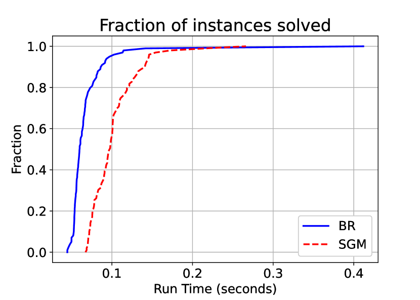
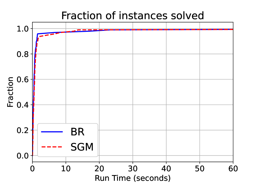
In the two player case, we observe that we are competitive with SGM. Figure 2(a) compares the performance profile of our algorithm with SGM. The BR algorithm presented in Algorithm 1 is slightly faster than SGM. The mean run-time for BR is 0.0683 seconds as oppossed to the mean run-time for SGM being 0.1017 seconds. The median run-time for BR is 0.0599 seconds, while the median run-time for SGM is 0.0971 seconds. This is consistent with the mild speed up discussed before. However, the mild is statistically significant that a paired t-test between the run time of the algorithms testing equality of means, the null hypothesis can be rejected with a p-value of $2.683\times 10^{-11}$ .

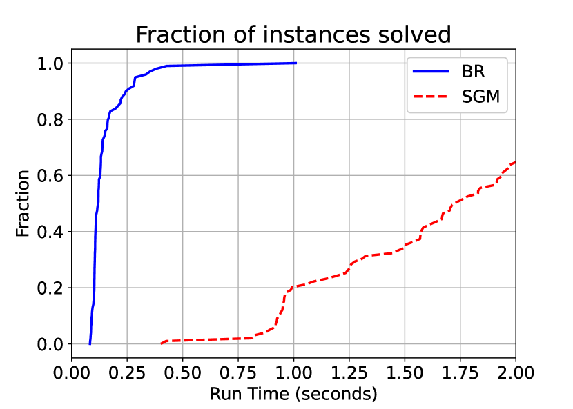
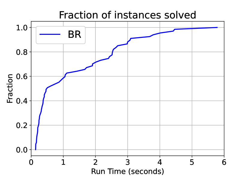
However, with three players, there is a considerable speed up when using the BR algorithm. The performance profile is depicted in Figure 2(b). We can see that almost all the instances were solved in less than 0.5 seconds when using BR, while almost no instance is solved within that time in SGM. Comparably, the mean run-time for BR and SGM in this set of instances is 0.1506 seconds and 3.3608 seconds. The median run-time for BR and SGM are 0.1192 and 1.7239 seconds, indicating that our algorithm is clearly at least ten times faster than SGM.

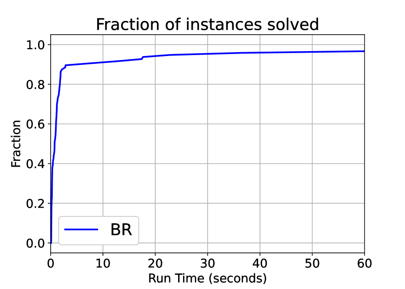
With four and five players, the difference is even more pronounced. The mean run-time for BR in the four and five player cases are 0.6087 seconds and 0.7477 seconds. The median run-time for BR in the four and five player cases are 0.5407 seconds and 0.6772 seconds. The SGM was run on these instances with a maximum allotted time of 120 seconds. We observe that not even one of the four-player instance or five-player instance was solved within 120 seconds, hinting at at least that our algorithm provides 100-times speed up when applicable.

Finally, we also note that in each of the 240 instances, the BR algorithm always terminated after finding a PNE or an MNE, but never a $\Delta$ -MNE with $\Delta>0$ (after allowing for numerical tolerance of $1\times 10^{-6}$ ). We share the instance-by-instance data on run time and the number of iterations in Appendix E in the electronic companion.

5.2 Random instances

Family description.

In this family of instances, the matrices ${\color[rgb]{0,0,0}\definecolor[named]{pgfstrokecolor}{rgb}{0,0,0}\pgfsys@color@gray@stroke{0}\pgfsys@color@gray@fill{0}{\mathbf{Q}}_{i}},{\color[rgb]{0,0,0}\definecolor[named]{pgfstrokecolor}{rgb}{0,0,0}\pgfsys@color@gray@stroke{0}\pgfsys@color@gray@fill{0}{\mathbf{d}}_{i}},{\color[rgb]{0,0,0}\definecolor[named]{pgfstrokecolor}{rgb}{0,0,0}\pgfsys@color@gray@stroke{0}\pgfsys@color@gray@fill{0}{\mathbf{C}}_{i}}$ are all randomly generated matrices with integer entries. To enure that ${\color[rgb]{0,0,0}\definecolor[named]{pgfstrokecolor}{rgb}{0,0,0}\pgfsys@color@gray@stroke{0}\pgfsys@color@gray@fill{0}{\mathbf{Q}}_{i}}$ s are positive definition, we generate a random integer matrix $P$ , and compute $\widetilde{{\color[rgb]{0,0,0}\definecolor[named]{pgfstrokecolor}{rgb}{0,0,0}\pgfsys@color@gray@stroke{0}\pgfsys@color@gray@fill{0}{\mathbf{Q}}_{i}}}=PP^{\top}$ , which is now guaranteed to be a positive-definite matrix with integer entries. Next, to ensure that the players have positively adequate objectives, we compute $\widetilde{{\color[rgb]{0,0,0}\definecolor[named]{pgfstrokecolor}{rgb}{0,0,0}\pgfsys@color@gray@stroke{0}\pgfsys@color@gray@fill{0}{\mathbf{R}}_{i}}}=\widetilde{{\color[rgb]{0,0,0}\definecolor[named]{pgfstrokecolor}{rgb}{0,0,0}\pgfsys@color@gray@stroke{0}\pgfsys@color@gray@fill{0}{\mathbf{Q}}_{i}}}^{-1}{\color[rgb]{0,0,0}\definecolor[named]{pgfstrokecolor}{rgb}{0,0,0}\pgfsys@color@gray@stroke{0}\pgfsys@color@gray@fill{0}{\mathbf{C}}_{i}}$ and compute the largest singular value of $\widetilde{{\color[rgb]{0,0,0}\definecolor[named]{pgfstrokecolor}{rgb}{0,0,0}\pgfsys@color@gray@stroke{0}\pgfsys@color@gray@fill{0}{\mathbf{R}}_{i}}}$ , which we denote as $\widetilde{\sigma_{1}}$ . Finally, we define ${\color[rgb]{0,0,0}\definecolor[named]{pgfstrokecolor}{rgb}{0,0,0}\pgfsys@color@gray@stroke{0}\pgfsys@color@gray@fill{0}{\mathbf{Q}}_{i}}=\left\lceil\sigma_{1}\right\rceil\widetilde{{\color[rgb]{0,0,0}\definecolor[named]{pgfstrokecolor}{rgb}{0,0,0}\pgfsys@color@gray@stroke{0}\pgfsys@color@gray@fill{0}{\mathbf{Q}}_{i}}}+\mathbf{I}$ . The ceiling ensures that ${\color[rgb]{0,0,0}\definecolor[named]{pgfstrokecolor}{rgb}{0,0,0}\pgfsys@color@gray@stroke{0}\pgfsys@color@gray@fill{0}{\mathbf{Q}}_{i}}$ has integer entries and the addition with the identity matrix ensures that we have each of the singular values of ${\color[rgb]{0,0,0}\definecolor[named]{pgfstrokecolor}{rgb}{0,0,0}\pgfsys@color@gray@stroke{0}\pgfsys@color@gray@fill{0}{\mathbf{R}}_{i}}={\color[rgb]{0,0,0}\definecolor[named]{pgfstrokecolor}{rgb}{0,0,0}\pgfsys@color@gray@stroke{0}\pgfsys@color@gray@fill{0}{\mathbf{Q}}_{i}}^{-1}{\color[rgb]{0,0,0}\definecolor[named]{pgfstrokecolor}{rgb}{0,0,0}\pgfsys@color@gray@stroke{0}\pgfsys@color@gray@fill{0}{\mathbf{C}}_{i}}$ is strictly lesser than $1$ .

Instance generation.

We vary the number of players between two, three, four, and five. Further, for each of the above four situations, we consider the decision vector of each player to be vary from 5, 10, 15, 20 or 25 variables. For each of the combinations, for example, three player games with fifteen variables per player or five player games with five variables per player, we generate 20 instances randomly. This gives a total of $4\times 5\times 20=400$ instances. Along with the exact matrices defining these 400 instances, we also share the code used to generate them.

Results.

In all subfamilies of instances with two to five players, there were two to four instances in each setting where numerical instabilities called failure of both the BR as well as the SGM algorithm. These instances were discarded from the below analysis as both the algorithms failed in these instances.

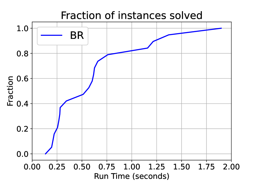
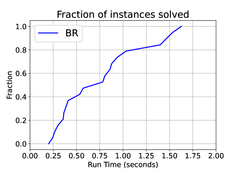
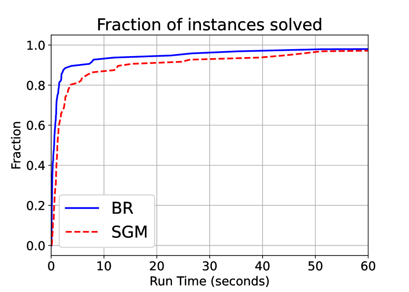
Out of the remaining instances, in the two player and three player cases, the performance of BR and SGM is comparable. In fact, we do not find any statistically significant difference between the two algorithms. Their performance profiles are plotted in Figures 3(a) and 3(b). However, when we have four or five players, the BR algorithm is significantly faster than the SGM algorithm. The BR always found a solution (except for the cases with numerical instabilities), with a median time of 5.348 seconds for four player-instances and 6.131 seconds for five player-instances, with the maximum time taken for any single instance being 233 seconds approximately. However, with the SGM algorithm, only eight of the hundred instances with four players were solved within a time limit of 500 seconds. The quickest one among them took over 290 seconds. Moreover, all eight solved instances are the simplest of the four player instances, where the decision vector of each player has five variables. Among the five player instances, only two of the hundred instances were solved within a time limit of 500 seconds, both of them taking over 400 seconds. Again, both the solved instances correspond to those where each player’s decision vector has five variables. The complete instance-by-instance details of the computational tests are presented in Appendix E in the electronic companion.

We also note that that, in every single instance that was solved (i.e., the ones that did not run into numerical error), the MNE of the restricted finite game after running the BR algorithm, had only a profitable deviation with maximum profit in the order of $10^{{-6}}$ , which can be considered as errors due to numerical methods used within the solver, thus motivating a conjecture that $\Delta=0$ is provable.

6 Future work

We end the paper with two possible avenues for future work. We first state a conjecture, which strengthens Corollary 1.

Conjecture 1.

Given an instance of ICQS with positively adequate objectives, and sets $S_{x}$ and $S_{y}$ from Algorithm 1, any MNE of the version of the game restricted to $S_{x}$ and $S_{y}$ is an MNE to ICQS.

In other words, the conjecture says that Corollary 1 holds with $\Delta_{x}=\Delta_{y}=0$ . The conjecture is validated by the computational experiments in Section 5. This is also consistent with the fact that the family of counterexamples provided in the proof of Theorem 4 do not have positively adequate objectives.

Second, the paper fundamentally uses the properties of quadratic functions to prove the results. It is conceivable then, that the results should hold even if the objective functions are approximated well by quadratic functions. For example, $L$ -Lipschitz, $\mu$ -strongly convex functions are both under-approximated and over-approximated by quadratic functions. However, an extension of these results to such functions and identifying the loss in the approximation ratios when considering such functions is non trivial, and is an interesting avenue for future work.

References

Adsul et al. (2021) Bharat Adsul, Jugal Garg, Ruta Mehta, Milind Sohoni, and Bernhard von Stengel. Fast algorithms for rank-1 bimatrix games. Operations Research, 69(2):613–631, March 2021. ISSN 1526-5463. doi: 10.1287/opre.2020.1981.
Audet et al. (2006) C. Audet, S. Belhaiza, and P. Hansen. Enumeration of All the Extreme Equilibria in Game Theory: Bimatrix and Polymatrix Games. Journal of Optimization Theory and Applications, 129(3):349–372, 2006. ISSN 0022-3239, 1573-2878. doi: 10.1007/s10957-006-9070-3. URL http://link.springer.com/10.1007/s10957-006-9070-3.
Ba and Pang (2022) Qin Ba and Jong-Shi Pang. Exact penalization of generalized nash equilibrium problems. Operations Research, 70(3):1448–1464, May 2022. ISSN 1526-5463. doi: 10.1287/opre.2019.1942.
Barvinok (2002) Alexander Barvinok. A course in convexity, volume 54. American Mathematical Soc., 2002.
Baudin and Laraki (2022) Lucas Baudin and Rida Laraki. Fictitious play and best-response dynamics in identical interest and zero-sum stochastic games. In International Conference on Machine Learning, pages 1664–1690. PMLR, 2022.
Bayer et al. (2023) Péter Bayer, György Kozics, and Nóra Gabriella Szőke. Best-response dynamics in directed network games. Journal of Economic Theory, 213:105720, 2023. ISSN 0022-0531. doi: 10.1016/j.jet.2023.105720.
Bichler et al. (2023) Martin Bichler, Max Fichtl, and Matthias Oberlechner. Computing bayes–nash equilibrium strategies in auction games via simultaneous online dual averaging. Operations Research, December 2023. ISSN 1526-5463. doi: 10.1287/opre.2022.0287.
Blom et al. (2022) Danny Blom, Bart Smeulders, and Frits C. R. Spieksma. Rejection-proof Kidney Exchange Mechanisms, 2022. URL https://arxiv.org/abs/2206.11525.
Carvalho et al. (2017) Margarida Carvalho, Andrea Lodi, João Pedro Pedroso, and Ana Viana. Nash equilibria in the two-player kidney exchange game. Mathematical Programming, 161(1-2):389–417, 2017. ISSN 0025-5610, 1436-4646. doi: 10.1007/s10107-016-1013-7.
Carvalho et al. (2022) Margarida Carvalho, Andrea Lodi, and João Pedro Pedroso. Computing equilibria for integer programming games. European Journal of Operational Research, 2022. ISSN 0377-2217.
Carvalho et al. (2023a) Margarida Carvalho, Gabriele Dragotto, Felipe Feijoo, Andrea Lodi, and Sriram Sankaranarayanan. When Nash meets Stackelberg. Management Science, 2023a. doi: 10.1287/mnsc.2022.03418.
Carvalho et al. (2023b) Margarida Carvalho, Gabriele Dragotto, Andrea Lodi, and Sriram Sankaranarayanan. The Cut and Play algorithm: Computing Nash equilibria via outer approximations. arXiv preprint arXiv:2111.05726, 2023b.
Carvalho et al. (2023c) Margarida Carvalho, Gabriele Dragotto, Andrea Lodi, and Sriram Sankaranarayanan. Integer programming games: A gentle computational overview. TutORials in Operations Research, 2023c.
Celaya et al. (2022) Marcel Celaya, Stefan Kuhlmann, Joseph Paat, and Robert Weismantel. Proximity and flatness bounds for linear integer optimization. arXiv preprint arXiv:2211.14941, 2022.
Cook et al. (1986) William Cook, Albertus MH Gerards, Alexander Schrijver, and Éva Tardos. Sensitivity theorems in integer linear programming. Mathematical Programming, 34:251–264, 1986.
Crönert and Minner (2022) Tobias Crönert and Stefan Minner. Equilibrium Identification and Selection in Finite Games. Operations Research, 2022. ISSN 0030-364X, 1526-5463. doi: 10.1287/opre.2022.2413.
Devine and Siddiqui (2023) Mel T Devine and Sauleh Siddiqui. Strategic investment decisions in an oligopoly with a competitive fringe: An equilibrium problem with equilibrium constraints approach. European Journal of Operational Research, 306(3):1473–1494, 2023.
Egging-Bratseth et al. (2020) Ruud Egging-Bratseth, Tobias Baltensperger, and Asgeir Tomasgard. Solving oligopolistic equilibrium problems with convex optimization. European Journal of Operational Research, 284(1):44–52, 2020.
Feijoo et al. (2018) Felipe Feijoo, Gokul C Iyer, Charalampos Avraam, Sauleh A Siddiqui, Leon E Clarke, Sriram Sankaranarayanan, Matthew T Binsted, Pralit L Patel, Nathalia C Prates, Evelyn Torres-Alfaro, et al. The future of natural gas infrastructure development in the united states. Applied energy, 228:149–166, 2018.
Feinstein and Rudloff (2023) Zachary Feinstein and Birgit Rudloff. Technical note—characterizing and computing the set of nash equilibria via vector optimization. Operations Research, May 2023. ISSN 1526-5463. doi: 10.1287/opre.2023.2457.
Granot and Skorin-Kapov (1990) Frieda Granot and Jadranka Skorin-Kapov. Some proximity and sensitivity results in quadratic integer programming. Mathematical Programming, 47(1-3):259–268, 1990.
Gurobi Optimization (2019) LLC Gurobi Optimization. Gurobi Optimizer Reference Manual, 2019. URL http://www.gurobi.com.
Hopkins (1999) Ed Hopkins. A note on best response dynamics. Games and Economic Behavior, 29(1-2):138–150, 1999.
Horn and Johnson (2012) Roger A Horn and Charles R Johnson. Matrix analysis. Cambridge university press, 2012.
Köppe et al. (2011) Matthias Köppe, Christopher Thomas Ryan, and Maurice Queyranne. Rational Generating Functions and Integer Programming Games. Operations Research, 59(6):1445–1460, 2011. ISSN 0030-364X, 1526-5463.
Kukushkin (2004) Nikolai S Kukushkin. Best response dynamics in finite games with additive aggregation. Games and Economic Behavior, 48(1):94–110, 2004.
Lamas and Chevalier (2018) Alejandro Lamas and Philippe Chevalier. Joint dynamic pricing and lot-sizing under competition. European Journal of Operational Research, 266(3):864–876, 2018. ISSN 0377-2217. doi: 10.1016/j.ejor.2017.10.026.
Langer et al. (2016) Lissy Langer, Daniel Huppmann, and Franziska Holz. Lifting the us crude oil export ban: A numerical partial equilibrium analysis. Energy Policy, 97:258–266, 2016.
Lei and Shanbhag (2022) Jinlong Lei and Uday V Shanbhag. Distributed variable sample-size gradient-response and best-response schemes for stochastic nash equilibrium problems. SIAM Journal on Optimization, 32(2):573–603, 2022.
Lemke and Howson (1964) C. E. Lemke and J. T. Howson, Jr. Equilibrium Points of Bimatrix Games. Journal of the Society for Industrial and Applied Mathematics, 12(2):413–423, 1964. ISSN 0368-4245, 2168-3484.
Leslie et al. (2020) David S Leslie, Steven Perkins, and Zibo Xu. Best-response dynamics in zero-sum stochastic games. Journal of Economic Theory, 189:105095, 2020.
Luna et al. (2023) Juan Pablo Luna, Claudia Sagastizábal, Julia Filiberti, Steven A. Gabriel, and Mikhail V. Solodov. Regularized equilibrium problems with equilibrium constraints with application to energy markets. SIAM Journal on Optimization, 33(3):1767–1796, 2023. doi: 10.1137/20M1353538.
Micciancio and Voulgaris (2013) Daniele Micciancio and Panagiotis Voulgaris. A deterministic single exponential time algorithm for most lattice problems based on voronoi cell computations. SIAM Journal on Computing, 42(3):1364–1391, 2013. doi: 10.1137/100811970.
Monderer and Shapley (1996) Dov Monderer and Lloyd S Shapley. Potential games. Games and economic behavior, 14(1):124–143, 1996.
Morgenstern and Von Neumann (1953) Oskar Morgenstern and John Von Neumann. Theory of games and economic behavior. Princeton university press, 1953.
Moriguchi et al. (2011) Satoko Moriguchi, Akiyoshi Shioura, and Nobuyuki Tsuchimura. M-convex function minimization by continuous relaxation approach: Proximity theorem and algorithm. SIAM Journal on Optimization, 21(3):633–668, 2011.
Morris (2003) Stephen Morris. Best response equivalence, 2003. Nach Informationen von SSRN wurde die ursprüngliche Fassung des Dokuments July 2002 erstellt.
Nash (1950) John F. Nash. Equilibrium Points in n-Person Games. Proceedings of the National Academy of Sciences of the United States of America, 36(1):48–49, 1950.
Nash (1951) John F. Nash. Non-Cooperative Games. The Annals of Mathematics, 54(2):286, 1951. ISSN 0003486X. doi: 10.2307/1969529.
Paat et al. (2020) Joseph Paat, Robert Weismantel, and Stefan Weltge. Distances between optimal solutions of mixed-integer programs. Mathematical Programming, 179(1-2):455–468, 2020.
Ravner and Snitkovsky (2023) Liron Ravner and Ran I. Snitkovsky. Stochastic approximation of symmetric nash equilibria in queueing games. Operations Research, June 2023. ISSN 1526-5463. doi: 10.1287/opre.2021.0306.
Rudelson (2000) M Rudelson. Distances between non-symmetric convex bodies and the-estimate. Positivity, 4(2):161–178, 2000.
Sandholm et al. (2005a) Thomas Sandholm, Andrew Gilpin, and Vincent Conitzer. Mixed-Integer Programming Methods for Finding Nash Equilibria. In Proceedings of the 20th National Conference on Artificial Intelligence - Volume 2, AAAI’05, pages 495–501. AAAI Press, 2005a. ISBN 1-57735-236-X. URL https://dl.acm.org/doi/10.5555/1619410.1619413.
Sandholm et al. (2005b) Tuomas Sandholm, Andrew Gilpin, and Vincent Conitzer. Mixed-integer programming methods for finding Nash equilibria. In AAAI, pages 495–501, 2005b.
Schwarze and Stein (2023) Stefan Schwarze and Oliver Stein. A branch-and-prune algorithm for discrete Nash equilibrium problems. Computational Optimization and Applications, pages 1–29, 2023.
Von Neumann and Morgenstern (1944) John Von Neumann and Oskar Morgenstern. Theory of Games and Economic Behavior. Princeton University Press, 1944. ISBN 978-1-4008-2946-0. doi: 10.1515/9781400829460.
Voorneveld (2000) Mark Voorneveld. Best-response potential games. Economics Letters, 66(3):289–295, 2000. ISSN 0165-1765. doi: 10.1016/S0165-1765(99)00196-2.
Wang et al. (2021) Chong Wang, Ping Ju, Feng Wu, Shunbo Lei, and Xueping Pan. Best response-based individually look-ahead scheduling for natural gas and power systems. Applied Energy, 304:117673, 2021.

Appendix A Continuous Quadratic Games

Definition 7 (Continuous convex quadratic Simultaneous game (CG-Nash)).

A Continuous Convex Quadratic Simultaneous game (CCQS) is a game of the form

\displaystyle\textbf{$\mathbf{x}$-player:}\min_{\mathbf{x}\in\mathbb{R}^{n_{x}}}:\frac{1}{2}\mathbf{x}^{\top}{\color[rgb]{0,0,0}\definecolor[named]{pgfstrokecolor}{rgb}{0,0,0}\pgfsys@color@gray@stroke{0}\pgfsys@color@gray@fill{0}{\mathbf{Q}}_{1}}\mathbf{x}+({\color[rgb]{0,0,0}\definecolor[named]{pgfstrokecolor}{rgb}{0,0,0}\pgfsys@color@gray@stroke{0}\pgfsys@color@gray@fill{0}{\mathbf{C}}_{1}}\mathbf{y}+{\color[rgb]{0,0,0}\definecolor[named]{pgfstrokecolor}{rgb}{0,0,0}\pgfsys@color@gray@stroke{0}\pgfsys@color@gray@fill{0}{\mathbf{d}}_{1}})^{\top}\mathbf{x}\qquad\qquad\textbf{$\mathbf{y}$-player:}\min_{\mathbf{y}\in\mathbb{R}^{n_{y}}}:\frac{1}{2}\mathbf{y}^{\top}{\color[rgb]{0,0,0}\definecolor[named]{pgfstrokecolor}{rgb}{0,0,0}\pgfsys@color@gray@stroke{0}\pgfsys@color@gray@fill{0}{\mathbf{Q}}_{2}}\mathbf{y}+({\color[rgb]{0,0,0}\definecolor[named]{pgfstrokecolor}{rgb}{0,0,0}\pgfsys@color@gray@stroke{0}\pgfsys@color@gray@fill{0}{\mathbf{C}}_{2}}\mathbf{x}+{\color[rgb]{0,0,0}\definecolor[named]{pgfstrokecolor}{rgb}{0,0,0}\pgfsys@color@gray@stroke{0}\pgfsys@color@gray@fill{0}{\mathbf{d}}_{2}})^{\top}\mathbf{y}

(CCQS)

Now, we present the results for this section.

Theorem 7.

If the game CCQS has negatively adequate objectives, there exist initial points $\widehat{\mathbf{x}}^{0},\widehat{\mathbf{y}}^{0}$ , starting from which Algorithm 1 generates divergent iterates, .

Theorem 8.

If the game CCQS has positively adequate objectives, then, irrespective of the initial points $\widehat{\mathbf{x}}^{0},\widehat{\mathbf{y}}^{0}$ , Algorithm 1 generates iterates converging to a PNE.

Theorems 7 and 8 above can be interpreted as necessary and sufficient conditions for Algorithm 1 converge to a PNE of CCQS. Theorem 7 only talks about existence of initial points starting from which the iterates will diverge, because, for example, one could start Algorithm 1 right at a PNE of the problem. And by the definition of PNE, the algorithm will terminate immediately. Nevertheless, the proof provides a constructive procedure to identify initial points so that Algorithm 1 is guaranteed to diverge.

For ease of exposition, we first prove Theorem 8 and then prove Theorem 7.

Proof of Theorem 8. .

Consider the best response ${\color[rgb]{0,0,0}\definecolor[named]{pgfstrokecolor}{rgb}{0,0,0}\pgfsys@color@gray@stroke{0}\pgfsys@color@gray@fill{0}{\color[rgb]{0,0,0}\definecolor[named]{pgfstrokecolor}{rgb}{0,0,0}\pgfsys@color@gray@stroke{0}\pgfsys@color@gray@fill{0}\mathcal{B}}_{1}\left(\mathbf{y}\right)}$ and ${\color[rgb]{0,0,0}\definecolor[named]{pgfstrokecolor}{rgb}{0,0,0}\pgfsys@color@gray@stroke{0}\pgfsys@color@gray@fill{0}{\color[rgb]{0,0,0}\definecolor[named]{pgfstrokecolor}{rgb}{0,0,0}\pgfsys@color@gray@stroke{0}\pgfsys@color@gray@fill{0}\mathcal{B}}_{2}\left(\mathbf{x}\right)}$ for both the players. There is a unique best response, since ${\color[rgb]{0,0,0}\definecolor[named]{pgfstrokecolor}{rgb}{0,0,0}\pgfsys@color@gray@stroke{0}\pgfsys@color@gray@fill{0}{\mathbf{Q}}_{1}}$ and ${\color[rgb]{0,0,0}\definecolor[named]{pgfstrokecolor}{rgb}{0,0,0}\pgfsys@color@gray@stroke{0}\pgfsys@color@gray@fill{0}{\mathbf{Q}}_{2}}$ are positive definite. The corresponding conditions for optimality are


$\displaystyle\mathbf{x}^{*}(\mathbf{y})\quad$	$\displaystyle=\quad-{\color[rgb]{0,0,0}\definecolor[named]{pgfstrokecolor}{rgb}{0,0,0}\pgfsys@color@gray@stroke{0}\pgfsys@color@gray@fill{0}{\mathbf{Q}}_{1}}^{-1}\left({\color[rgb]{0,0,0}\definecolor[named]{pgfstrokecolor}{rgb}{0,0,0}\pgfsys@color@gray@stroke{0}\pgfsys@color@gray@fill{0}{\mathbf{C}}_{1}}\mathbf{y}+{\color[rgb]{0,0,0}\definecolor[named]{pgfstrokecolor}{rgb}{0,0,0}\pgfsys@color@gray@stroke{0}\pgfsys@color@gray@fill{0}{\mathbf{d}}_{1}}\right)$	(9a)
$\displaystyle\mathbf{y}^{*}(\mathbf{x})\quad$	$\displaystyle=\quad-{\color[rgb]{0,0,0}\definecolor[named]{pgfstrokecolor}{rgb}{0,0,0}\pgfsys@color@gray@stroke{0}\pgfsys@color@gray@fill{0}{\mathbf{Q}}_{2}}^{-1}\left({\color[rgb]{0,0,0}\definecolor[named]{pgfstrokecolor}{rgb}{0,0,0}\pgfsys@color@gray@stroke{0}\pgfsys@color@gray@fill{0}{\mathbf{C}}_{2}}\mathbf{x}+{\color[rgb]{0,0,0}\definecolor[named]{pgfstrokecolor}{rgb}{0,0,0}\pgfsys@color@gray@stroke{0}\pgfsys@color@gray@fill{0}{\mathbf{d}}_{2}}\right)$	(9b)

So, in case we follow the best-response iteration, the successive iterates can be obtained by the updates defined in 9. This can be seen as the fixed-point iteration of the function


$\displaystyle F\begin{pmatrix}{}\mathbf{x}{}\\ {}\mathbf{y}{}\end{pmatrix}\quad$	$\displaystyle=\quad\left(\begin{array}[]{c}-{\color[rgb]{0,0,0}\definecolor[named]{pgfstrokecolor}{rgb}{0,0,0}\pgfsys@color@gray@stroke{0}\pgfsys@color@gray@fill{0}{\mathbf{Q}}_{1}}^{-1}\left({\color[rgb]{0,0,0}\definecolor[named]{pgfstrokecolor}{rgb}{0,0,0}\pgfsys@color@gray@stroke{0}\pgfsys@color@gray@fill{0}{\mathbf{C}}_{1}}\mathbf{y}+{\color[rgb]{0,0,0}\definecolor[named]{pgfstrokecolor}{rgb}{0,0,0}\pgfsys@color@gray@stroke{0}\pgfsys@color@gray@fill{0}{\mathbf{d}}_{1}}\right)\\ -{\color[rgb]{0,0,0}\definecolor[named]{pgfstrokecolor}{rgb}{0,0,0}\pgfsys@color@gray@stroke{0}\pgfsys@color@gray@fill{0}{\mathbf{Q}}_{2}}^{-1}\left({\color[rgb]{0,0,0}\definecolor[named]{pgfstrokecolor}{rgb}{0,0,0}\pgfsys@color@gray@stroke{0}\pgfsys@color@gray@fill{0}{\mathbf{C}}_{2}}\mathbf{x}+{\color[rgb]{0,0,0}\definecolor[named]{pgfstrokecolor}{rgb}{0,0,0}\pgfsys@color@gray@stroke{0}\pgfsys@color@gray@fill{0}{\mathbf{d}}_{2}}\right)\end{array}\right)$	(10c)
	$\displaystyle=\quad\begin{pmatrix}\mathbf{0}&-{\color[rgb]{0,0,0}\definecolor[named]{pgfstrokecolor}{rgb}{0,0,0}\pgfsys@color@gray@stroke{0}\pgfsys@color@gray@fill{0}{\mathbf{R}}_{1}}\\ -{\color[rgb]{0,0,0}\definecolor[named]{pgfstrokecolor}{rgb}{0,0,0}\pgfsys@color@gray@stroke{0}\pgfsys@color@gray@fill{0}{\mathbf{R}}_{2}}&\mathbf{0}\end{pmatrix}\begin{pmatrix}{}\mathbf{x}{}\\ {}\mathbf{y}{}\end{pmatrix}+\begin{pmatrix}{\color[rgb]{0,0,0}\definecolor[named]{pgfstrokecolor}{rgb}{0,0,0}\pgfsys@color@gray@stroke{0}\pgfsys@color@gray@fill{0}{\mathbf{Q}}_{1}}^{-1}{\color[rgb]{0,0,0}\definecolor[named]{pgfstrokecolor}{rgb}{0,0,0}\pgfsys@color@gray@stroke{0}\pgfsys@color@gray@fill{0}{\mathbf{d}}_{1}}\\ {\color[rgb]{0,0,0}\definecolor[named]{pgfstrokecolor}{rgb}{0,0,0}\pgfsys@color@gray@stroke{0}\pgfsys@color@gray@fill{0}{\mathbf{Q}}_{2}}^{-1}{\color[rgb]{0,0,0}\definecolor[named]{pgfstrokecolor}{rgb}{0,0,0}\pgfsys@color@gray@stroke{0}\pgfsys@color@gray@fill{0}{\mathbf{d}}_{2}}\end{pmatrix}$	(10d)

Let us analyse how $F$ maps two points, and the norm of the difference of the images of those points. We observe


	$\displaystyle\left\\|F\begin{pmatrix}\mathbf{x}^{1}\\ \mathbf{y}^{1}\end{pmatrix}-F\begin{pmatrix}\mathbf{x}^{2}\\ \mathbf{y}^{2}\end{pmatrix}\right\\|\quad$	$\displaystyle=\quad\left\\|\left(\begin{pmatrix}\mathbf{0}&-{\color[rgb]{0,0,0}\definecolor[named]{pgfstrokecolor}{rgb}{0,0,0}\pgfsys@color@gray@stroke{0}\pgfsys@color@gray@fill{0}{\mathbf{R}}_{1}}\\ -{\color[rgb]{0,0,0}\definecolor[named]{pgfstrokecolor}{rgb}{0,0,0}\pgfsys@color@gray@stroke{0}\pgfsys@color@gray@fill{0}{\mathbf{R}}_{2}}&\mathbf{0}\end{pmatrix}\begin{pmatrix}\mathbf{x}^{1}\\ \mathbf{y}^{1}\end{pmatrix}+\begin{pmatrix}{\color[rgb]{0,0,0}\definecolor[named]{pgfstrokecolor}{rgb}{0,0,0}\pgfsys@color@gray@stroke{0}\pgfsys@color@gray@fill{0}{\mathbf{Q}}_{1}}^{-1}{\color[rgb]{0,0,0}\definecolor[named]{pgfstrokecolor}{rgb}{0,0,0}\pgfsys@color@gray@stroke{0}\pgfsys@color@gray@fill{0}{\mathbf{d}}_{1}}\\ {\color[rgb]{0,0,0}\definecolor[named]{pgfstrokecolor}{rgb}{0,0,0}\pgfsys@color@gray@stroke{0}\pgfsys@color@gray@fill{0}{\mathbf{Q}}_{2}}^{-1}{\color[rgb]{0,0,0}\definecolor[named]{pgfstrokecolor}{rgb}{0,0,0}\pgfsys@color@gray@stroke{0}\pgfsys@color@gray@fill{0}{\mathbf{d}}_{2}}\end{pmatrix}\right)\right.$
		$\displaystyle\qquad\qquad\left.-\left(\begin{pmatrix}\mathbf{0}&-{\color[rgb]{0,0,0}\definecolor[named]{pgfstrokecolor}{rgb}{0,0,0}\pgfsys@color@gray@stroke{0}\pgfsys@color@gray@fill{0}{\mathbf{R}}_{1}}\\ -{\color[rgb]{0,0,0}\definecolor[named]{pgfstrokecolor}{rgb}{0,0,0}\pgfsys@color@gray@stroke{0}\pgfsys@color@gray@fill{0}{\mathbf{R}}_{2}}&\mathbf{0}\end{pmatrix}\begin{pmatrix}\mathbf{x}^{2}\\ \mathbf{y}^{2}\end{pmatrix}+\begin{pmatrix}{\color[rgb]{0,0,0}\definecolor[named]{pgfstrokecolor}{rgb}{0,0,0}\pgfsys@color@gray@stroke{0}\pgfsys@color@gray@fill{0}{\mathbf{Q}}_{1}}^{-1}{\color[rgb]{0,0,0}\definecolor[named]{pgfstrokecolor}{rgb}{0,0,0}\pgfsys@color@gray@stroke{0}\pgfsys@color@gray@fill{0}{\mathbf{d}}_{1}}\\ {\color[rgb]{0,0,0}\definecolor[named]{pgfstrokecolor}{rgb}{0,0,0}\pgfsys@color@gray@stroke{0}\pgfsys@color@gray@fill{0}{\mathbf{Q}}_{2}}^{-1}{\color[rgb]{0,0,0}\definecolor[named]{pgfstrokecolor}{rgb}{0,0,0}\pgfsys@color@gray@stroke{0}\pgfsys@color@gray@fill{0}{\mathbf{d}}_{2}}\end{pmatrix}\right)\right\\|$
		$\displaystyle=\quad\left\\|\begin{pmatrix}\mathbf{0}&-{\color[rgb]{0,0,0}\definecolor[named]{pgfstrokecolor}{rgb}{0,0,0}\pgfsys@color@gray@stroke{0}\pgfsys@color@gray@fill{0}{\mathbf{R}}_{1}}\\ -{\color[rgb]{0,0,0}\definecolor[named]{pgfstrokecolor}{rgb}{0,0,0}\pgfsys@color@gray@stroke{0}\pgfsys@color@gray@fill{0}{\mathbf{R}}_{2}}&\mathbf{0}\end{pmatrix}\begin{pmatrix}\mathbf{x}^{1}-\mathbf{x}^{2}\\ \mathbf{y}^{1}-\mathbf{y}^{2}\end{pmatrix}\right\\|$
		$\displaystyle=\quad\left\\|-\begin{pmatrix}{\color[rgb]{0,0,0}\definecolor[named]{pgfstrokecolor}{rgb}{0,0,0}\pgfsys@color@gray@stroke{0}\pgfsys@color@gray@fill{0}{\mathbf{R}}_{1}}&\mathbf{0}\\ \mathbf{0}&{\color[rgb]{0,0,0}\definecolor[named]{pgfstrokecolor}{rgb}{0,0,0}\pgfsys@color@gray@stroke{0}\pgfsys@color@gray@fill{0}{\mathbf{R}}_{2}}\end{pmatrix}\begin{pmatrix}\mathbf{y}^{1}-\mathbf{y}^{2}\\ \mathbf{x}^{1}-\mathbf{x}^{2}\end{pmatrix}\right\\|$
		$\displaystyle<\quad\left\\|\begin{pmatrix}\mathbf{x}^{1}\\ \mathbf{y}^{1}\end{pmatrix}-\begin{pmatrix}\mathbf{x}^{2}\\ \mathbf{y}^{2}\end{pmatrix}\right\\|$

where the inequality in the last step follows due to the fact that the largest singular value of $\begin{pmatrix}{\color[rgb]{0,0,0}\definecolor[named]{pgfstrokecolor}{rgb}{0,0,0}\pgfsys@color@gray@stroke{0}\pgfsys@color@gray@fill{0}{\mathbf{R}}_{1}}&\mathbf{0}\\ \mathbf{0}&{\color[rgb]{0,0,0}\definecolor[named]{pgfstrokecolor}{rgb}{0,0,0}\pgfsys@color@gray@stroke{0}\pgfsys@color@gray@fill{0}{\mathbf{R}}_{2}}\end{pmatrix}$ is at most the largest singular value of ${\color[rgb]{0,0,0}\definecolor[named]{pgfstrokecolor}{rgb}{0,0,0}\pgfsys@color@gray@stroke{0}\pgfsys@color@gray@fill{0}{\mathbf{R}}_{1}}$ and ${\color[rgb]{0,0,0}\definecolor[named]{pgfstrokecolor}{rgb}{0,0,0}\pgfsys@color@gray@stroke{0}\pgfsys@color@gray@fill{0}{\mathbf{R}}_{2}}$ (Proposition 1) and this is at most $1$ since we have positively adequate objectives and finally Proposition 2 gives the inequality.

Thus, we have established $\left\|F\begin{pmatrix}\mathbf{x}^{1}\\ \mathbf{y}^{1}\end{pmatrix}-F\begin{pmatrix}\mathbf{x}^{2}\\ \mathbf{y}^{2}\end{pmatrix}\right\|<\left\|\begin{pmatrix}\mathbf{x}^{1}\\ \mathbf{y}^{1}\end{pmatrix}-\begin{pmatrix}\mathbf{x}^{2}\\ \mathbf{y}^{2}\end{pmatrix}\right\|$ for any arbitrary vectors. But, this means that $F$ is a contractive mapping. It is known that the fixed-point iteration converges to a fixed-point if the mapping is contractive. But a fixed point in this context means two successive iterates in Algorithm 1 adapted for CCQS. Thus the algorithm will terminate in pure-strategy condition, and the fixed point is a PNE for CCQS. ∎

Now, we will prove Theorem 7.

Proof of Theorem 7. .

Let every singular value of ${\color[rgb]{0,0,0}\definecolor[named]{pgfstrokecolor}{rgb}{0,0,0}\pgfsys@color@gray@stroke{0}\pgfsys@color@gray@fill{0}{\mathbf{R}}_{1}}$ and ${\color[rgb]{0,0,0}\definecolor[named]{pgfstrokecolor}{rgb}{0,0,0}\pgfsys@color@gray@stroke{0}\pgfsys@color@gray@fill{0}{\mathbf{R}}_{2}}$ be at least $1+\rho$ with $\rho>0$ . We use the fixed-point iteration of the function $F$ defined in 10. Since this tracks the iterations of Algorithm 1, if we show that this fixed-point iteration diverges, so does Algorithm 1. We observe that

	$\displaystyle F\begin{pmatrix}\mathbf{x}\\ \mathbf{y}\end{pmatrix}\quad$	$\displaystyle=\quad\begin{pmatrix}\mathbf{0}&-{\color[rgb]{0,0,0}\definecolor[named]{pgfstrokecolor}{rgb}{0,0,0}\pgfsys@color@gray@stroke{0}\pgfsys@color@gray@fill{0}{\mathbf{R}}_{1}}\\ -{\color[rgb]{0,0,0}\definecolor[named]{pgfstrokecolor}{rgb}{0,0,0}\pgfsys@color@gray@stroke{0}\pgfsys@color@gray@fill{0}{\mathbf{R}}_{2}}&\mathbf{0}\end{pmatrix}\begin{pmatrix}{}\mathbf{x}{}\\ {}\mathbf{y}{}\end{pmatrix}+\begin{pmatrix}{\color[rgb]{0,0,0}\definecolor[named]{pgfstrokecolor}{rgb}{0,0,0}\pgfsys@color@gray@stroke{0}\pgfsys@color@gray@fill{0}{\mathbf{Q}}_{1}}^{-1}{\color[rgb]{0,0,0}\definecolor[named]{pgfstrokecolor}{rgb}{0,0,0}\pgfsys@color@gray@stroke{0}\pgfsys@color@gray@fill{0}{\mathbf{d}}_{1}}\\ {\color[rgb]{0,0,0}\definecolor[named]{pgfstrokecolor}{rgb}{0,0,0}\pgfsys@color@gray@stroke{0}\pgfsys@color@gray@fill{0}{\mathbf{Q}}_{2}}^{-1}{\color[rgb]{0,0,0}\definecolor[named]{pgfstrokecolor}{rgb}{0,0,0}\pgfsys@color@gray@stroke{0}\pgfsys@color@gray@fill{0}{\mathbf{d}}_{2}}\end{pmatrix}$
	$\displaystyle\implies\left\\|F\begin{pmatrix}\mathbf{x}\\ \mathbf{y}\end{pmatrix}-\begin{pmatrix}{\color[rgb]{0,0,0}\definecolor[named]{pgfstrokecolor}{rgb}{0,0,0}\pgfsys@color@gray@stroke{0}\pgfsys@color@gray@fill{0}{\mathbf{Q}}_{1}}^{-1}{\color[rgb]{0,0,0}\definecolor[named]{pgfstrokecolor}{rgb}{0,0,0}\pgfsys@color@gray@stroke{0}\pgfsys@color@gray@fill{0}{\mathbf{d}}_{1}}\\ {\color[rgb]{0,0,0}\definecolor[named]{pgfstrokecolor}{rgb}{0,0,0}\pgfsys@color@gray@stroke{0}\pgfsys@color@gray@fill{0}{\mathbf{Q}}_{2}}^{-1}{\color[rgb]{0,0,0}\definecolor[named]{pgfstrokecolor}{rgb}{0,0,0}\pgfsys@color@gray@stroke{0}\pgfsys@color@gray@fill{0}{\mathbf{d}}_{2}}\end{pmatrix}\right\\|\quad$	$\displaystyle=\quad\left\\|\begin{pmatrix}\mathbf{0}&-{\color[rgb]{0,0,0}\definecolor[named]{pgfstrokecolor}{rgb}{0,0,0}\pgfsys@color@gray@stroke{0}\pgfsys@color@gray@fill{0}{\mathbf{R}}_{1}}\\ -{\color[rgb]{0,0,0}\definecolor[named]{pgfstrokecolor}{rgb}{0,0,0}\pgfsys@color@gray@stroke{0}\pgfsys@color@gray@fill{0}{\mathbf{R}}_{2}}&\mathbf{0}\end{pmatrix}\begin{pmatrix}{}\mathbf{x}{}\\ {}\mathbf{y}{}\end{pmatrix}\right\\|$
	$\displaystyle\implies\left\\|F\begin{pmatrix}{}\mathbf{x}{}\\ {}\mathbf{y}{}\end{pmatrix}\right\\|+\left\\|\begin{pmatrix}{\color[rgb]{0,0,0}\definecolor[named]{pgfstrokecolor}{rgb}{0,0,0}\pgfsys@color@gray@stroke{0}\pgfsys@color@gray@fill{0}{\mathbf{Q}}_{1}}^{-1}{\color[rgb]{0,0,0}\definecolor[named]{pgfstrokecolor}{rgb}{0,0,0}\pgfsys@color@gray@stroke{0}\pgfsys@color@gray@fill{0}{\mathbf{d}}_{1}}\\ {\color[rgb]{0,0,0}\definecolor[named]{pgfstrokecolor}{rgb}{0,0,0}\pgfsys@color@gray@stroke{0}\pgfsys@color@gray@fill{0}{\mathbf{Q}}_{2}}^{-1}{\color[rgb]{0,0,0}\definecolor[named]{pgfstrokecolor}{rgb}{0,0,0}\pgfsys@color@gray@stroke{0}\pgfsys@color@gray@fill{0}{\mathbf{d}}_{2}}\end{pmatrix}\right\\|\quad$	$\displaystyle>\quad\left(1+\rho\right)\left\\|\begin{pmatrix}{}\mathbf{x}{}\\ {}\mathbf{y}{}\end{pmatrix}\right\\|$
where the inequality holds because the singular value of the matrix in the RHS above are all at least as large as the smallest singular value of ${\color[rgb]{0,0,0}\definecolor[named]{pgfstrokecolor}{rgb}{0,0,0}\pgfsys@color@gray@stroke{0}\pgfsys@color@gray@fill{0}{\mathbf{R}}_{1}}$ and ${\color[rgb]{0,0,0}\definecolor[named]{pgfstrokecolor}{rgb}{0,0,0}\pgfsys@color@gray@stroke{0}\pgfsys@color@gray@fill{0}{\mathbf{R}}_{2}}$ , which are at least $(1+\rho)$ , and then by applying Proposition 2.
	$\displaystyle\implies\left\\|F\begin{pmatrix}{}\mathbf{x}{}\\ {}\mathbf{y}{}\end{pmatrix}\right\\|\quad$	$\displaystyle>\quad\left(1+\rho\right)\left\\|\begin{pmatrix}{}\mathbf{x}{}\\ {}\mathbf{y}{}\end{pmatrix}\right\\|-\left\\|\begin{pmatrix}{\color[rgb]{0,0,0}\definecolor[named]{pgfstrokecolor}{rgb}{0,0,0}\pgfsys@color@gray@stroke{0}\pgfsys@color@gray@fill{0}{\mathbf{Q}}_{1}}^{-1}{\color[rgb]{0,0,0}\definecolor[named]{pgfstrokecolor}{rgb}{0,0,0}\pgfsys@color@gray@stroke{0}\pgfsys@color@gray@fill{0}{\mathbf{d}}_{1}}\\ {\color[rgb]{0,0,0}\definecolor[named]{pgfstrokecolor}{rgb}{0,0,0}\pgfsys@color@gray@stroke{0}\pgfsys@color@gray@fill{0}{\mathbf{Q}}_{2}}^{-1}{\color[rgb]{0,0,0}\definecolor[named]{pgfstrokecolor}{rgb}{0,0,0}\pgfsys@color@gray@stroke{0}\pgfsys@color@gray@fill{0}{\mathbf{d}}_{2}}\end{pmatrix}\right\\|$
where the inequalities are due to negatively adequate objectives and Propositions 2 and 1. Now, if $\left\\|\begin{pmatrix}{}\mathbf{x}{}\\ {}\mathbf{y}{}\end{pmatrix}\right\\|>\frac{\left\\|\begin{pmatrix}{\color[rgb]{0,0,0}\definecolor[named]{pgfstrokecolor}{rgb}{0,0,0}\pgfsys@color@gray@stroke{0}\pgfsys@color@gray@fill{0}{\mathbf{Q}}_{1}}^{-1}{\color[rgb]{0,0,0}\definecolor[named]{pgfstrokecolor}{rgb}{0,0,0}\pgfsys@color@gray@stroke{0}\pgfsys@color@gray@fill{0}{\mathbf{d}}_{1}}\\ {\color[rgb]{0,0,0}\definecolor[named]{pgfstrokecolor}{rgb}{0,0,0}\pgfsys@color@gray@stroke{0}\pgfsys@color@gray@fill{0}{\mathbf{Q}}_{2}}^{-1}{\color[rgb]{0,0,0}\definecolor[named]{pgfstrokecolor}{rgb}{0,0,0}\pgfsys@color@gray@stroke{0}\pgfsys@color@gray@fill{0}{\mathbf{d}}_{2}}\end{pmatrix}\right\\|}{\rho}$ , then the above becomes
	$\displaystyle\left\\|F\begin{pmatrix}{}\mathbf{x}{}\\ {}\mathbf{y}{}\end{pmatrix}\right\\|\quad$	$\displaystyle>\quad\left\\|\begin{pmatrix}{}\mathbf{x}{}\\ {}\mathbf{y}{}\end{pmatrix}\right\\|$

But this means that the iterates are going successively get farther and farther from the origin, and any arbitrarily large norm bound will be eventually crossed to never return back and repeat any iterate. This indicates that Algorithm 1 as adapted for CCQS will diverge. ∎

Appendix B Extension for multiple players

Suppose there are multiple players $1,\dots,k$ . We denote the variables of player $i$ as $\mathbf{x}^{i}$ and those of everybody except $i$ as $\mathbf{x}^{-i}$ . Now, the objective function if player $i$ is given as $\frac{1}{2}{\mathbf{x}^{i}}^{\top}{\color[rgb]{0,0,0}\definecolor[named]{pgfstrokecolor}{rgb}{0,0,0}\pgfsys@color@gray@stroke{0}\pgfsys@color@gray@fill{0}{\mathbf{Q}}_{i}}\mathbf{x}^{i}+\left({\color[rgb]{0,0,0}\definecolor[named]{pgfstrokecolor}{rgb}{0,0,0}\pgfsys@color@gray@stroke{0}\pgfsys@color@gray@fill{0}{\mathbf{C}}_{i}}\mathbf{x}^{-i}+{\color[rgb]{0,0,0}\definecolor[named]{pgfstrokecolor}{rgb}{0,0,0}\pgfsys@color@gray@stroke{0}\pgfsys@color@gray@fill{0}{\mathbf{d}}_{i}}\right)^{\top}\mathbf{x}^{i}$ . For example, in a three player game, suppose the objective function of player $1$ is given as $\frac{1}{2}{\mathbf{x}^{1}}^{\top}{\color[rgb]{0,0,0}\definecolor[named]{pgfstrokecolor}{rgb}{0,0,0}\pgfsys@color@gray@stroke{0}\pgfsys@color@gray@fill{0}{\mathbf{Q}}_{1}}\mathbf{x}^{1}+\left({\color[rgb]{0,0,0}\definecolor[named]{pgfstrokecolor}{rgb}{0,0,0}\pgfsys@color@gray@stroke{0}\pgfsys@color@gray@fill{0}{\mathbf{C}}_{1,2}}\mathbf{x}^{2}+{\color[rgb]{0,0,0}\definecolor[named]{pgfstrokecolor}{rgb}{0,0,0}\pgfsys@color@gray@stroke{0}\pgfsys@color@gray@fill{0}{\mathbf{C}}_{1,3}}\mathbf{x}^{3}+{\color[rgb]{0,0,0}\definecolor[named]{pgfstrokecolor}{rgb}{0,0,0}\pgfsys@color@gray@stroke{0}\pgfsys@color@gray@fill{0}{\mathbf{d}}_{1}}\right)^{\top}\mathbf{x}^{1}$ , we write ${\color[rgb]{0,0,0}\definecolor[named]{pgfstrokecolor}{rgb}{0,0,0}\pgfsys@color@gray@stroke{0}\pgfsys@color@gray@fill{0}{\mathbf{C}}_{1}}=\begin{pmatrix}{\color[rgb]{0,0,0}\definecolor[named]{pgfstrokecolor}{rgb}{0,0,0}\pgfsys@color@gray@stroke{0}\pgfsys@color@gray@fill{0}{\mathbf{C}}_{1,2}}&{\color[rgb]{0,0,0}\definecolor[named]{pgfstrokecolor}{rgb}{0,0,0}\pgfsys@color@gray@stroke{0}\pgfsys@color@gray@fill{0}{\mathbf{C}}_{1,3}}\end{pmatrix}$ . Thus, ${\color[rgb]{0,0,0}\definecolor[named]{pgfstrokecolor}{rgb}{0,0,0}\pgfsys@color@gray@stroke{0}\pgfsys@color@gray@fill{0}{\mathbf{C}}_{1}}\mathbf{x}^{-1}=\begin{pmatrix}{\color[rgb]{0,0,0}\definecolor[named]{pgfstrokecolor}{rgb}{0,0,0}\pgfsys@color@gray@stroke{0}\pgfsys@color@gray@fill{0}{\mathbf{C}}_{1,2}}&{\color[rgb]{0,0,0}\definecolor[named]{pgfstrokecolor}{rgb}{0,0,0}\pgfsys@color@gray@stroke{0}\pgfsys@color@gray@fill{0}{\mathbf{C}}_{1,3}}\end{pmatrix}\begin{pmatrix}\mathbf{x}^{2}\\ \mathbf{x}^{3}\end{pmatrix}={\color[rgb]{0,0,0}\definecolor[named]{pgfstrokecolor}{rgb}{0,0,0}\pgfsys@color@gray@stroke{0}\pgfsys@color@gray@fill{0}{\mathbf{C}}_{1,2}}\mathbf{x}^{2}+{\color[rgb]{0,0,0}\definecolor[named]{pgfstrokecolor}{rgb}{0,0,0}\pgfsys@color@gray@stroke{0}\pgfsys@color@gray@fill{0}{\mathbf{C}}_{1,3}}\mathbf{x}^{3}$ .

The successive iterates, as in the proof of Theorem 1, are given by $\mathbf{x}^{i,t+1}\leftarrow-{\color[rgb]{0,0,0}\definecolor[named]{pgfstrokecolor}{rgb}{0,0,0}\pgfsys@color@gray@stroke{0}\pgfsys@color@gray@fill{0}{\mathbf{Q}}_{i}}^{-1}({\color[rgb]{0,0,0}\definecolor[named]{pgfstrokecolor}{rgb}{0,0,0}\pgfsys@color@gray@stroke{0}\pgfsys@color@gray@fill{0}{\mathbf{C}}_{i}}\mathbf{x}^{-i,t}+{\color[rgb]{0,0,0}\definecolor[named]{pgfstrokecolor}{rgb}{0,0,0}\pgfsys@color@gray@stroke{0}\pgfsys@color@gray@fill{0}{\mathbf{d}}_{i}})+z_{i}(\mathbf{x}^{-i,t})$ . The index $i$ refers to the player whose best response is being computed and $t$ refers to the iteration number.

We provide a proof sketch that even with $k$ players, a theorem analogous to that of Theorem 1 holds. In other words, when the game has positively adequate objectives, then the best-response algorithm terminates. Now, analogous to the proof of Theorem 1, we can write the difference between two strategy profiles as $\left\|\begin{pmatrix}\mathbf{x}^{1,t+1}\\ \vdots\\ \mathbf{x}^{k,t+1}\end{pmatrix}\right\|=\left\|\begin{pmatrix}-{\color[rgb]{0,0,0}\definecolor[named]{pgfstrokecolor}{rgb}{0,0,0}\pgfsys@color@gray@stroke{0}\pgfsys@color@gray@fill{0}{\mathbf{Q}}_{1}}^{-1}({\color[rgb]{0,0,0}\definecolor[named]{pgfstrokecolor}{rgb}{0,0,0}\pgfsys@color@gray@stroke{0}\pgfsys@color@gray@fill{0}{\mathbf{C}}_{1}}\mathbf{x}^{-1,t}+{\color[rgb]{0,0,0}\definecolor[named]{pgfstrokecolor}{rgb}{0,0,0}\pgfsys@color@gray@stroke{0}\pgfsys@color@gray@fill{0}{\mathbf{d}}_{1}})+z_{1}(\mathbf{x}^{-1,t})\\ \vdots\\ -{\color[rgb]{0,0,0}\definecolor[named]{pgfstrokecolor}{rgb}{0,0,0}\pgfsys@color@gray@stroke{0}\pgfsys@color@gray@fill{0}{\mathbf{Q}}_{k}}^{-k}({\color[rgb]{0,0,0}\definecolor[named]{pgfstrokecolor}{rgb}{0,0,0}\pgfsys@color@gray@stroke{0}\pgfsys@color@gray@fill{0}{\mathbf{C}}_{k}}\mathbf{x}^{-k,t}+{\color[rgb]{0,0,0}\definecolor[named]{pgfstrokecolor}{rgb}{0,0,0}\pgfsys@color@gray@stroke{0}\pgfsys@color@gray@fill{0}{\mathbf{d}}_{k}})+z_{k}(\mathbf{x}^{-k,t})\end{pmatrix}\right\|=\left\|\begin{pmatrix}(-{\color[rgb]{0,0,0}\definecolor[named]{pgfstrokecolor}{rgb}{0,0,0}\pgfsys@color@gray@stroke{0}\pgfsys@color@gray@fill{0}{\mathbf{R}}_{1}}\mathbf{x}^{-1,t}-{\color[rgb]{0,0,0}\definecolor[named]{pgfstrokecolor}{rgb}{0,0,0}\pgfsys@color@gray@stroke{0}\pgfsys@color@gray@fill{0}{\mathbf{Q}}_{1}}^{-1}{\color[rgb]{0,0,0}\definecolor[named]{pgfstrokecolor}{rgb}{0,0,0}\pgfsys@color@gray@stroke{0}\pgfsys@color@gray@fill{0}{\mathbf{d}}_{1}})+z_{1}(\mathbf{x}^{-1,t})\\ \vdots\\ (-{\color[rgb]{0,0,0}\definecolor[named]{pgfstrokecolor}{rgb}{0,0,0}\pgfsys@color@gray@stroke{0}\pgfsys@color@gray@fill{0}{\mathbf{R}}_{k}}\mathbf{x}^{-k,t}+-{\color[rgb]{0,0,0}\definecolor[named]{pgfstrokecolor}{rgb}{0,0,0}\pgfsys@color@gray@stroke{0}\pgfsys@color@gray@fill{0}{\mathbf{Q}}_{k}}^{-k}{\color[rgb]{0,0,0}\definecolor[named]{pgfstrokecolor}{rgb}{0,0,0}\pgfsys@color@gray@stroke{0}\pgfsys@color@gray@fill{0}{\mathbf{d}}_{k}})+z_{k}(\mathbf{x}^{-k,t})\end{pmatrix}\right\|\leq\left\|\begin{pmatrix}{\color[rgb]{0,0,0}\definecolor[named]{pgfstrokecolor}{rgb}{0,0,0}\pgfsys@color@gray@stroke{0}\pgfsys@color@gray@fill{0}{\mathbf{R}}_{1}}&\cdots&0\\ \vdots&\ddots&\vdots\\ 0&\cdots&{\color[rgb]{0,0,0}\definecolor[named]{pgfstrokecolor}{rgb}{0,0,0}\pgfsys@color@gray@stroke{0}\pgfsys@color@gray@fill{0}{\mathbf{R}}_{k}}\end{pmatrix}\right\|\left\|\begin{pmatrix}\mathbf{x}^{1,t}\\ \vdots\\ \mathbf{x}^{k,t}\end{pmatrix}\right\|+\left\|\begin{pmatrix}{\color[rgb]{0,0,0}\definecolor[named]{pgfstrokecolor}{rgb}{0,0,0}\pgfsys@color@gray@stroke{0}\pgfsys@color@gray@fill{0}{\mathbf{Q}}_{1}}^{-1}{\color[rgb]{0,0,0}\definecolor[named]{pgfstrokecolor}{rgb}{0,0,0}\pgfsys@color@gray@stroke{0}\pgfsys@color@gray@fill{0}{\mathbf{d}}_{1}}\\ \vdots\\ {\color[rgb]{0,0,0}\definecolor[named]{pgfstrokecolor}{rgb}{0,0,0}\pgfsys@color@gray@stroke{0}\pgfsys@color@gray@fill{0}{\mathbf{Q}}_{k}}^{-1}{\color[rgb]{0,0,0}\definecolor[named]{pgfstrokecolor}{rgb}{0,0,0}\pgfsys@color@gray@stroke{0}\pgfsys@color@gray@fill{0}{\mathbf{d}}_{k}}\end{pmatrix}\right\|+\left\|\begin{pmatrix}z_{1}(\mathbf{x}^{-1,t})\\ \vdots\\ z_{k}(\mathbf{x}^{-k,t})\end{pmatrix}\right\|\leq(1-\rho)\left\|\begin{pmatrix}\begin{pmatrix}\mathbf{x}^{1,t}\\ \vdots\\ \mathbf{x}^{k,t}\end{pmatrix}\end{pmatrix}\right\|+\left\|\begin{pmatrix}{\color[rgb]{0,0,0}\definecolor[named]{pgfstrokecolor}{rgb}{0,0,0}\pgfsys@color@gray@stroke{0}\pgfsys@color@gray@fill{0}{\mathbf{Q}}_{1}}^{-1}{\color[rgb]{0,0,0}\definecolor[named]{pgfstrokecolor}{rgb}{0,0,0}\pgfsys@color@gray@stroke{0}\pgfsys@color@gray@fill{0}{\mathbf{d}}_{1}}\\ \vdots\\ {\color[rgb]{0,0,0}\definecolor[named]{pgfstrokecolor}{rgb}{0,0,0}\pgfsys@color@gray@stroke{0}\pgfsys@color@gray@fill{0}{\mathbf{Q}}_{k}}^{-1}{\color[rgb]{0,0,0}\definecolor[named]{pgfstrokecolor}{rgb}{0,0,0}\pgfsys@color@gray@stroke{0}\pgfsys@color@gray@fill{0}{\mathbf{d}}_{k}}\end{pmatrix}\right\|+\left\|\begin{pmatrix}{\color[rgb]{0,0,0}\definecolor[named]{pgfstrokecolor}{rgb}{0,0,0}\pgfsys@color@gray@stroke{0}\pgfsys@color@gray@fill{0}{\color[rgb]{0,0,0}\definecolor[named]{pgfstrokecolor}{rgb}{0,0,0}\pgfsys@color@gray@stroke{0}\pgfsys@color@gray@fill{0}\pi}\left({\color[rgb]{0,0,0}\definecolor[named]{pgfstrokecolor}{rgb}{0,0,0}\pgfsys@color@gray@stroke{0}\pgfsys@color@gray@fill{0}{\mathbf{Q}}_{1}}\right)}\\ \vdots\\ {\color[rgb]{0,0,0}\definecolor[named]{pgfstrokecolor}{rgb}{0,0,0}\pgfsys@color@gray@stroke{0}\pgfsys@color@gray@fill{0}{\color[rgb]{0,0,0}\definecolor[named]{pgfstrokecolor}{rgb}{0,0,0}\pgfsys@color@gray@stroke{0}\pgfsys@color@gray@fill{0}\pi}\left({\color[rgb]{0,0,0}\definecolor[named]{pgfstrokecolor}{rgb}{0,0,0}\pgfsys@color@gray@stroke{0}\pgfsys@color@gray@fill{0}{\mathbf{Q}}_{k}}\right)}\end{pmatrix}\right\|$ . Like before, we observe that if the norm of $\left\|\begin{pmatrix}\begin{pmatrix}\mathbf{x}^{1,t}\\ \vdots\\ \mathbf{x}^{k,t}\end{pmatrix}\end{pmatrix}\right\|$ is large, then the iterate in the subsequent iteration will necessarily have a smaller norm. But this means, the iterates will have to return to a bounded region, if they begin to move towards infinity. But in any bounded region, there will be finitely many feasible integer points, leading to cycling and hence termination. Hence the proof.

Next, it is straightforward to observe Theorem 5 translates to multiplayer case naturally. The proof of Theorem 5 considers the strategies of player $\mathbf{x}$ , while using the probabilities and strategies of player $\mathbf{y}$ . In a multi-player setting, the same proof can be adapted, by considering all the other players’s strategies $\mathbf{x}^{-i}$ , when establishing a bound $\Delta_{i}$ .

Finally, to provide the bounds on $L_{x}$ (which will now be notated as $L_{i}$ when there are multiple players), we express 7g in terms of $L_{-i}$ , which is the maximum distance between two valid $\mathbf{x}^{-i}$ that appears in the cycle.

Appendix C Auxiliary results

We state these auxiliary results for ready reference. The following results are available (typically in greater generality) in most standard texts on matrix analysis, for example, Horn and Johnson (2012). However, a short proof sketch is provided for the reader’s convenience.

Proposition 1.

Let $\mathbf{A}$ be an $m\times n$ matrix and $\mathbf{B}$ be an $n\times m$ matrix. Let $\sigma^{A}_{1},\dots,\sigma^{A}_{k}$ be the singular values of $\mathbf{A}$ and $\sigma^{B}_{1},\dots,\sigma^{B}_{\ell}$ be the singular values of $\mathbf{B}$ . Then, the singular values of the $(m+n)\times(m+n)$ matrix $\begin{pmatrix}\mathbf{A}&\mathbf{0}\\ \mathbf{0}&\mathbf{B}\end{pmatrix}$ are $\sigma^{A}_{1},\dots,\sigma^{A}_{k},\sigma^{B}_{1},\dots,\sigma^{B}_{\ell}$ .

Proof of Proposition 1..

Consider the singular value decompositions (SVD) of matrices $\mathbf{A}$ and $\mathbf{B}$ . Let $\mathbf{A}=\mathbf{U}^{A}\mathbf{\Sigma}^{A}\mathbf{V}^{A}$ and $\mathbf{B}=\mathbf{U}^{B}\mathbf{\Sigma}^{B}\mathbf{V}^{B}$ . Then, $\mathbf{C}:=\begin{pmatrix}\mathbf{A}&\mathbf{0}\\ \mathbf{0}&\mathbf{B}\end{pmatrix}=\mathbf{U}\mathbf{\Sigma}^{\prime}\mathbf{V}=\begin{pmatrix}\mathbf{U}^{A}&\mathbf{0}\\ \mathbf{0}&\mathbf{U}^{B}\end{pmatrix}\begin{pmatrix}\mathbf{\Sigma}^{A}&\mathbf{0}\\ \mathbf{0}&\mathbf{\Sigma}^{B}\end{pmatrix}\begin{pmatrix}\mathbf{V}^{A}&\mathbf{0}\\ \mathbf{0}&\mathbf{V}^{B}\end{pmatrix}$ , which is obtained by muiltiplying the block matrices. While $\mathbf{\Sigma}^{\prime}$ is not diagonal, its rows and columns can be permuted according to a permutation matrix $\mathbf{P}$ to get $\mathbf{\Sigma}^{\prime}=\mathbf{P}\mathbf{\Sigma}\mathbf{P}^{\top}$ to get $\mathbf{C}=(\mathbf{U}\mathbf{P})\mathbf{\Sigma}(\mathbf{P}^{\top}\mathbf{V})$ where the only non-zero elements of $\mathbf{\Sigma}$ are along its diagonal. It can also be verified that $\mathbf{U}\mathbf{P}$ and $\mathbf{P}^{\top}\mathbf{V}$ are unitary, completing the proof. The only non-zero elements of $\mathbf{\Sigma}$ are the singular values of $\mathbf{A}$ and $\mathbf{B}$ , making them the singular values of $\mathbf{C}$ . ∎

Proposition 2.

Every singular value of a matrix $M$ is strictly lesser than $1$ if and only if $\left\|\mathbf{M}\mathbf{x}\right\|_{2}<\left\|\mathbf{x}\right\|_{2}$ for every $\mathbf{x}\in\mathbb{R}^{n}$ . Every singular value of a matrix $M$ is strictly greater than $1$ if and only if $\left\|\mathbf{M}\mathbf{x}\right\|_{2}>\left\|\mathbf{x}\right\|_{2}$ for every $\mathbf{x}\in\mathbb{R}^{n}$ .

Proof of Proposition 2..

Let $\mathbf{M}$ be a matrix of dimension $m\times n$ with real entries. Then, the singular values of $\mathbf{M}$ are the square roots of the eigenvalues of $\mathbf{M}^{\top}\mathbf{M}$ . Let us call this matrix $\mathbf{M}^{\prime}$ . Since $\mathbf{M}^{\prime}$ is symmetric, all its eigen values are real. Moreover, from Rayleigh’s theorem, the largest value that $\mathbf{x}^{\top}\mathbf{M}^{\prime}\mathbf{x}$ can take is $\overline{\lambda}\mathbf{x}^{\top}\mathbf{x}$ and the smallest value it can take is $\underline{\lambda}\mathbf{x}^{\top}\mathbf{x}$ where $\overline{\lambda}$ and $\underline{\lambda}$ are the largest and the smallest eigen values of $\mathbf{M}^{\prime}$ respectively. Now, observe $\left\|\mathbf{M}\mathbf{x}\right\|^{2}_{2}=\mathbf{x}^{\top}\mathbf{M}^{\top}\mathbf{M}\mathbf{x}=\mathbf{x}^{\top}\mathbf{M}^{\prime}\mathbf{x}\leq\overline{\lambda}\left\|\mathbf{x}\right\|^{2}_{2}$ . But the largest eigen value of $\mathbf{M}^{\prime}$ , which is $\overline{\lambda}$ , is the square of the largest singular value of $\mathbf{M}$ (denoted as $\sigma_{1}$ ). Thus, we have $\left\|\mathbf{M}\mathbf{x}\right\|^{2}_{2}\leq\sigma_{1}^{2}\left\|\mathbf{x}\right\|^{2}_{2}$ , which implies $\left\|\mathbf{M}\mathbf{x}\right\|_{2}\leq\sigma_{1}\left\|\mathbf{x}\right\|_{2}$ . This proves the first part of the result. The second part can be proved using analogous arguments. ∎

Appendix D Discussion on the rate of convergence.

In the context of both CCQS and ICQS, it is important to bound the number of iterations taken by Algorithm 1 before termination. We discuss this when the game has positively adequate objectives, and hence termination is guaranteed. Like in case of descent algorithms for continuous nonlinear programs, the number of iterations is sensitive to the initial point.

We note that when we have positively adequate objectives, then the iterates converge to the neighborhood of the region where cycling occurs. In particular, we show the following. Let $S_{x}\times S_{y}$ be a set about which cycling can possibly occur. Then, iterates will move towards a neighborhood around this set at a linearly convergent rate.

More formally, we state the same as follows. Let $\left(\widehat{\mathbf{x}}^{i},\widehat{\mathbf{y}}^{i}\right)$ be some iterate generated by Algorithm 1. Let $(\mathbf{x}^{i*},\mathbf{y}^{i*})\in S_{x}\times S_{y}$ be the point in $S_{x}\times S_{y}$ that is closest to $\left(\widehat{\mathbf{x}}^{i},\widehat{\mathbf{y}}^{i}\right)$ . If $\left\|\begin{pmatrix}\widehat{\mathbf{x}}^{i}\\ \widehat{\mathbf{y}}^{i}\end{pmatrix}-\begin{pmatrix}\mathbf{x}^{i*}\\ \mathbf{y}^{i*}\end{pmatrix}\right\|>\frac{2{\color[rgb]{0,0,0}\definecolor[named]{pgfstrokecolor}{rgb}{0,0,0}\pgfsys@color@gray@stroke{0}\pgfsys@color@gray@fill{0}\pi}_{\left\|\cdot\right\|}}{\varepsilon}$ for some $0<\varepsilon<\rho$ , then we claim that $\left\|\begin{pmatrix}\widehat{\mathbf{x}}^{i+1}\\ \widehat{\mathbf{y}}^{i+1}\end{pmatrix}-\begin{pmatrix}\mathbf{x}^{(i+1)*}\\ \mathbf{y}^{(i+1)*}\end{pmatrix}\right\|<(1-\rho+\varepsilon)\left\|\begin{pmatrix}\widehat{\mathbf{x}}^{i}\\ \widehat{\mathbf{y}}^{i}\end{pmatrix}-\begin{pmatrix}\mathbf{x}^{i*}\\ \mathbf{y}^{i*}\end{pmatrix}\right\|$ . In other words, if the iterate is at least $2{\color[rgb]{0,0,0}\definecolor[named]{pgfstrokecolor}{rgb}{0,0,0}\pgfsys@color@gray@stroke{0}\pgfsys@color@gray@fill{0}\pi}_{\left\|\cdot\right\|}/\varepsilon$ away from any point in $S_{x}$ , then there is a linear rate of convergence towards the neighborhood.

The reasoning behind this is as follows. As argued earlier, if the game ICQS has positively adequate objectives, then the matrix $\begin{pmatrix}\mathbf{0}&-{\color[rgb]{0,0,0}\definecolor[named]{pgfstrokecolor}{rgb}{0,0,0}\pgfsys@color@gray@stroke{0}\pgfsys@color@gray@fill{0}{\mathbf{R}}_{1}}\\ -{\color[rgb]{0,0,0}\definecolor[named]{pgfstrokecolor}{rgb}{0,0,0}\pgfsys@color@gray@stroke{0}\pgfsys@color@gray@fill{0}{\mathbf{R}}_{2}}&\mathbf{0}\end{pmatrix}$ has all its singular values less than $1$ strictly. In particular, let each of them be less than or equal to $1-\rho$ for some $\rho>0$ . Let ${\color[rgb]{0,0,0}\definecolor[named]{pgfstrokecolor}{rgb}{0,0,0}\pgfsys@color@gray@stroke{0}\pgfsys@color@gray@fill{0}\pi}_{\left\|\cdot\right\|}:={\left\|\begin{pmatrix}{\color[rgb]{0,0,0}\definecolor[named]{pgfstrokecolor}{rgb}{0,0,0}\pgfsys@color@gray@stroke{0}\pgfsys@color@gray@fill{0}{\color[rgb]{0,0,0}\definecolor[named]{pgfstrokecolor}{rgb}{0,0,0}\pgfsys@color@gray@stroke{0}\pgfsys@color@gray@fill{0}\pi}\left({\color[rgb]{0,0,0}\definecolor[named]{pgfstrokecolor}{rgb}{0,0,0}\pgfsys@color@gray@stroke{0}\pgfsys@color@gray@fill{0}{\mathbf{Q}}_{1}}\right)}\\ {\color[rgb]{0,0,0}\definecolor[named]{pgfstrokecolor}{rgb}{0,0,0}\pgfsys@color@gray@stroke{0}\pgfsys@color@gray@fill{0}{\color[rgb]{0,0,0}\definecolor[named]{pgfstrokecolor}{rgb}{0,0,0}\pgfsys@color@gray@stroke{0}\pgfsys@color@gray@fill{0}\pi}\left({\color[rgb]{0,0,0}\definecolor[named]{pgfstrokecolor}{rgb}{0,0,0}\pgfsys@color@gray@stroke{0}\pgfsys@color@gray@fill{0}{\mathbf{Q}}_{2}}\right)}\end{pmatrix}\right\|}$ . Further, let $F:\mathbb{R}^{n_{x}+n_{y}}\to\mathbb{R}^{n_{x}+n_{y}}$ be as defined in 3d, mapping each iterate in the best-response iteration to the next iterate. Now,


	$\displaystyle\left\\|\begin{pmatrix}\widehat{\mathbf{x}}^{i+1}\\ \widehat{\mathbf{y}}^{i+1}\end{pmatrix}-\begin{pmatrix}\mathbf{x}^{(i+1)}\\ \mathbf{y}^{(i+1)}\end{pmatrix}\right\\|$	$\displaystyle\leq\left\\|\begin{pmatrix}\widehat{\mathbf{x}}^{i+1}\\ \widehat{\mathbf{y}}^{i+1}\end{pmatrix}-F\begin{pmatrix}\mathbf{x}^{i}\\ \mathbf{y}^{i}\end{pmatrix}\right\\|$
		$\displaystyle=\left\\|F\begin{pmatrix}\widehat{\mathbf{x}}^{i}\\ \widehat{\mathbf{y}}^{i}\end{pmatrix}-F\begin{pmatrix}\mathbf{x}^{i}\\ \mathbf{y}^{i}\end{pmatrix}\right\\|$
		$\displaystyle=\left\\|\begin{pmatrix}\mathbf{0}&-{\color[rgb]{0,0,0}\definecolor[named]{pgfstrokecolor}{rgb}{0,0,0}\pgfsys@color@gray@stroke{0}\pgfsys@color@gray@fill{0}{\mathbf{R}}_{1}}\\ -{\color[rgb]{0,0,0}\definecolor[named]{pgfstrokecolor}{rgb}{0,0,0}\pgfsys@color@gray@stroke{0}\pgfsys@color@gray@fill{0}{\mathbf{R}}_{2}}&\mathbf{0}\end{pmatrix}\begin{pmatrix}\widehat{\mathbf{x}}^{i}-\mathbf{x}^{i}\\ \widehat{\mathbf{y}}^{i}-\mathbf{y}^{i}\end{pmatrix}+\begin{pmatrix}\mathbf{z}_{x}(\widehat{\mathbf{x}}^{i})-\mathbf{z}_{x}(\mathbf{x}^{i})\\ \mathbf{z}_{y}(\widehat{\mathbf{y}}^{i})-\mathbf{z}_{y}(\mathbf{y}^{i})\end{pmatrix}\right\\|$
		$\displaystyle\leq\left\\|\begin{pmatrix}\mathbf{0}&-{\color[rgb]{0,0,0}\definecolor[named]{pgfstrokecolor}{rgb}{0,0,0}\pgfsys@color@gray@stroke{0}\pgfsys@color@gray@fill{0}{\mathbf{R}}_{1}}\\ -{\color[rgb]{0,0,0}\definecolor[named]{pgfstrokecolor}{rgb}{0,0,0}\pgfsys@color@gray@stroke{0}\pgfsys@color@gray@fill{0}{\mathbf{R}}_{2}}&\mathbf{0}\end{pmatrix}\begin{pmatrix}\widehat{\mathbf{x}}^{i}-\mathbf{x}^{i}\\ \widehat{\mathbf{y}}^{i}-\mathbf{y}^{i}\end{pmatrix}\right\\|+\left\\|\begin{pmatrix}\mathbf{z}_{x}(\widehat{\mathbf{x}}^{i})-\mathbf{z}_{x}(\mathbf{x}^{i})\\ \mathbf{z}_{y}(\widehat{\mathbf{y}}^{i})-\mathbf{z}_{y}(\mathbf{y}^{i})\end{pmatrix}\right\\|$
		$\displaystyle\leq\left\\|\begin{pmatrix}\mathbf{0}&-{\color[rgb]{0,0,0}\definecolor[named]{pgfstrokecolor}{rgb}{0,0,0}\pgfsys@color@gray@stroke{0}\pgfsys@color@gray@fill{0}{\mathbf{R}}_{1}}\\ -{\color[rgb]{0,0,0}\definecolor[named]{pgfstrokecolor}{rgb}{0,0,0}\pgfsys@color@gray@stroke{0}\pgfsys@color@gray@fill{0}{\mathbf{R}}_{2}}&\mathbf{0}\end{pmatrix}\begin{pmatrix}\widehat{\mathbf{x}}^{i}-\mathbf{x}^{i}\\ \widehat{\mathbf{y}}^{i}-\mathbf{y}^{i}\end{pmatrix}\right\\|+\left\\|\begin{pmatrix}\mathbf{z}_{x}(\widehat{\mathbf{x}}^{i})\\ \mathbf{z}_{y}(\widehat{\mathbf{y}}^{i})\end{pmatrix}\right\\|+\left\\|\begin{pmatrix}\mathbf{z}_{x}(\mathbf{x}^{i})\\ \mathbf{z}_{y}(\mathbf{y}^{i})\end{pmatrix}\right\\|$
		$\displaystyle\leq\left\\|\begin{pmatrix}\mathbf{0}&-{\color[rgb]{0,0,0}\definecolor[named]{pgfstrokecolor}{rgb}{0,0,0}\pgfsys@color@gray@stroke{0}\pgfsys@color@gray@fill{0}{\mathbf{R}}_{1}}\\ -{\color[rgb]{0,0,0}\definecolor[named]{pgfstrokecolor}{rgb}{0,0,0}\pgfsys@color@gray@stroke{0}\pgfsys@color@gray@fill{0}{\mathbf{R}}_{2}}&\mathbf{0}\end{pmatrix}\begin{pmatrix}\widehat{\mathbf{x}}^{i}-\mathbf{x}^{i}\\ \widehat{\mathbf{y}}^{i}-\mathbf{y}^{i}\end{pmatrix}\right\\|+2{\color[rgb]{0,0,0}\definecolor[named]{pgfstrokecolor}{rgb}{0,0,0}\pgfsys@color@gray@stroke{0}\pgfsys@color@gray@fill{0}\pi}_{\left\\|\cdot\right\\|}$
		$\displaystyle=\left\\|\begin{pmatrix}{\color[rgb]{0,0,0}\definecolor[named]{pgfstrokecolor}{rgb}{0,0,0}\pgfsys@color@gray@stroke{0}\pgfsys@color@gray@fill{0}{\mathbf{R}}_{1}}&\mathbf{0}\\ \mathbf{0}&{\color[rgb]{0,0,0}\definecolor[named]{pgfstrokecolor}{rgb}{0,0,0}\pgfsys@color@gray@stroke{0}\pgfsys@color@gray@fill{0}{\mathbf{R}}_{2}}\end{pmatrix}U\begin{pmatrix}\widehat{\mathbf{x}}^{i}-\mathbf{x}^{i}\\ \widehat{\mathbf{y}}^{i}-\mathbf{y}^{i}\end{pmatrix}\right\\|+2{\color[rgb]{0,0,0}\definecolor[named]{pgfstrokecolor}{rgb}{0,0,0}\pgfsys@color@gray@stroke{0}\pgfsys@color@gray@fill{0}\pi}_{\left\\|\cdot\right\\|}$
		$\displaystyle\leq(1-\rho)\left\\|\begin{pmatrix}\widehat{\mathbf{x}}^{i}-\mathbf{x}^{i}\\ \widehat{\mathbf{y}}^{i}-\mathbf{y}^{i}\end{pmatrix}\right\\|+2{\color[rgb]{0,0,0}\definecolor[named]{pgfstrokecolor}{rgb}{0,0,0}\pgfsys@color@gray@stroke{0}\pgfsys@color@gray@fill{0}\pi}_{\left\\|\cdot\right\\|}$
		$\displaystyle=(1-\rho+\varepsilon)\left\\|\begin{pmatrix}\widehat{\mathbf{x}}^{i}-\mathbf{x}^{i}\\ \widehat{\mathbf{y}}^{i}-\mathbf{y}^{i}\end{pmatrix}\right\\|-\varepsilon\left\\|\begin{pmatrix}\widehat{\mathbf{x}}^{i}-\mathbf{x}^{i}\\ \widehat{\mathbf{y}}^{i}-\mathbf{y}^{i}\end{pmatrix}\right\\|+2{\color[rgb]{0,0,0}\definecolor[named]{pgfstrokecolor}{rgb}{0,0,0}\pgfsys@color@gray@stroke{0}\pgfsys@color@gray@fill{0}\pi}_{\left\\|\cdot\right\\|}$
		$\displaystyle\leq(1-\rho+\varepsilon)\left\\|\begin{pmatrix}\widehat{\mathbf{x}}^{i}-\mathbf{x}^{i}\\ \widehat{\mathbf{y}}^{i}-\mathbf{y}^{i}\end{pmatrix}\right\\|$

Here, the first inequality follows from the fact that $\begin{pmatrix}\mathbf{x}^{(i+1)*}\\ \mathbf{y}^{(i+1)*}\end{pmatrix}$ is the closest point in $S_{x}\times S_{y}$ to $\begin{pmatrix}\widehat{\mathbf{x}}^{i+1}\\ \widehat{\mathbf{y}}^{i+1}\end{pmatrix}$ and that $F\begin{pmatrix}\mathbf{x}^{i*}\\ \mathbf{y}^{i*}\end{pmatrix}\in S_{x}\times S_{y}$ . The next equality is obtained from the fact that the consecutive iterates are generated by applying the function $F$ and the next equality is about substituting the function $F$ as per 3d. The following two inequalities are both by applying the trianguar inequality of norms. The next inequality is a consequence of Theorem 3 that the integer minimum is at a bounded distance away from the continuous minimum. The equality following that introduces a unitary matrix $U$ like before that reorders the rows of the vector as needed. The next inequality follows due to the assumption that the largest singular value of both ${\color[rgb]{0,0,0}\definecolor[named]{pgfstrokecolor}{rgb}{0,0,0}\pgfsys@color@gray@stroke{0}\pgfsys@color@gray@fill{0}{\mathbf{R}}_{1}}$ and ${\color[rgb]{0,0,0}\definecolor[named]{pgfstrokecolor}{rgb}{0,0,0}\pgfsys@color@gray@stroke{0}\pgfsys@color@gray@fill{0}{\mathbf{R}}_{2}}$ are at most $(1-\rho)$ . The next equality is obtained by adding and subtracting $\varepsilon\left\|\begin{pmatrix}\widehat{\mathbf{x}}^{i}-\mathbf{x}^{i*}\\ \widehat{\mathbf{y}}^{i}-\mathbf{y}^{i*}\end{pmatrix}\right\|$ on the RHS. The last inequality is true, if $2{\color[rgb]{0,0,0}\definecolor[named]{pgfstrokecolor}{rgb}{0,0,0}\pgfsys@color@gray@stroke{0}\pgfsys@color@gray@fill{0}\pi}_{\left\|\cdot\right\|}-\varepsilon\left\|\begin{pmatrix}\widehat{\mathbf{x}}^{i}-\mathbf{x}^{i*}\\ \widehat{\mathbf{y}}^{i}-\mathbf{y}^{i*}\end{pmatrix}\right\|\leq 0$ which is equivalent to say $\left\|\begin{pmatrix}\widehat{\mathbf{x}}^{i}-\mathbf{x}^{i*}\\ \widehat{\mathbf{y}}^{i}-\mathbf{y}^{i*}\end{pmatrix}\right\|\geq\frac{2{\color[rgb]{0,0,0}\definecolor[named]{pgfstrokecolor}{rgb}{0,0,0}\pgfsys@color@gray@stroke{0}\pgfsys@color@gray@fill{0}\pi}_{\left\|\cdot\right\|}}{\varepsilon}$ . In other words, as claimed, if the iterates are far away from the set $S_{x}\times S_{y}$ , then there is a linear rate of convergence. i.e., the distance goes down by a constant factor of $(1-\rho+\varepsilon)$ in each iteration. till the iterates reach a neighborhood of radius $2{\color[rgb]{0,0,0}\definecolor[named]{pgfstrokecolor}{rgb}{0,0,0}\pgfsys@color@gray@stroke{0}\pgfsys@color@gray@fill{0}\pi}_{\left\|\cdot\right\|}/\varepsilon$ around $S_{x}\times S_{y}$ . Following that, however, we believe that guarantees are not possible about when cycling could occur.

The same analysis also says that in the context of CCQS, where the term corresponding to $2{\color[rgb]{0,0,0}\definecolor[named]{pgfstrokecolor}{rgb}{0,0,0}\pgfsys@color@gray@stroke{0}\pgfsys@color@gray@fill{0}\pi}_{\left\|\cdot\right\|}$ is $0$ , linear convergence to the PNE is guaranteed.

Appendix E Computational experiments data

For the 240 instances of the pricing game with substitutes and complements and the 500 instances of the random games, we provide the run-time data here below. Each instance is recognized by the unique filename that has the data for the instance. The second column indicates the number of players in the instance. The third and fourth columns titled $t_{BR}$ and $t_{SGM}$ indicate the time taken by the BR and SGM algorithms respectively on the problem. An entry saying TL here indicates that the maximum time limit is reached but no MNE is found. An entry saying Num Err indicates that the solver ran into numerical issues as some of the matrices possibly have large entries in them. In particular, we state numerical error, if the integer programming solver (Gurobi) declares that the matrix ${\color[rgb]{0,0,0}\definecolor[named]{pgfstrokecolor}{rgb}{0,0,0}\pgfsys@color@gray@stroke{0}\pgfsys@color@gray@fill{0}{\mathbf{Q}}}$ used is not positive definite. This is not possible from construction, as the instances are generated by choosing ${\color[rgb]{0,0,0}\definecolor[named]{pgfstrokecolor}{rgb}{0,0,0}\pgfsys@color@gray@stroke{0}\pgfsys@color@gray@fill{0}{\mathbf{Q}}}=\mathbf{A}\mathbf{A}^{\top}+\mathbf{I}$ for some random $\mathbf{A}$ . However, some times, large entries in ${\color[rgb]{0,0,0}\definecolor[named]{pgfstrokecolor}{rgb}{0,0,0}\pgfsys@color@gray@stroke{0}\pgfsys@color@gray@fill{0}{\mathbf{Q}}}$ makes Gurobi to declare that the matrix is not positive definite, and we report numerical errors in these cases. Finally, the last two columns $k_{{BR}}$ and $k_{SGM}$ indicate the number of iterations of the BR and the SGM algorithms that ran before either successful termination or reaching the time limit or running into numerical issues.

E.1 Pricing with substitutes and complements

Instance name	nPlay	$t_{BR}$	$t_{SGM}$	$k_{BR}$	$k_{SGM}$
asymmMktGame_N2_1.json	2	0.2172	0.1425	4	6
asymmMktGame_N2_2.json	2	0.1812	0.1904	4	5
asymmMktGame_N2_3.json	2	0.3832	0.3613	5	7
asymmMktGame_N2_4.json	2	0.1808	0.2887	5	7
asymmMktGame_N2_5.json	2	0.3706	0.5868	4	5
asymmMktGame_N2_6.json	2	0.138	0.1444	4	5
asymmMktGame_N2_7.json	2	0.4024	0.9749	4	6
asymmMktGame_N2_8.json	2	0.2808	0.5777	4	5
asymmMktGame_N2_9.json	2	0.9021	0.5659	4	6
asymmMktGame_N2_10.json	2	0.1653	1.3944	4	6
asymmMktGame_N2_11.json	2	1.1006	0.3641	4	6
asymmMktGame_N2_12.json	2	0.1449	0.5067	4	6
asymmMktGame_N2_13.json	2	0.8202	0.9078	5	7
asymmMktGame_N2_14.json	2	1.4994	0.9507	4	5
asymmMktGame_N2_15.json	2	0.2634	0.1862	6	5
asymmMktGame_N2_16.json	2	0.1037	0.1353	4	5
asymmMktGame_N2_17.json	2	0.7951	2.0591	4	6
asymmMktGame_N2_18.json	2	1.4928	1.1661	4	6
asymmMktGame_N2_19.json	2	0.3455	1.1541	3	5
asymmMktGame_N2_20.json	2	0.5566	0.89	4	5
asymmMktGame_N2_21.json	2	0.5051	0.5074	4	5
asymmMktGame_N2_22.json	2	0.9255	0.3385	3	5
asymmMktGame_N2_23.json	2	1.8685	0.8177	4	6
asymmMktGame_N2_24.json	2	1.1305	0.9827	4	7
asymmMktGame_N2_25.json	2	0.3919	1.0244	4	7
asymmMktGame_N2_26.json	2	0.6474	0.5421	4	6
asymmMktGame_N2_27.json	2	0.3688	0.5998	4	6
asymmMktGame_N2_28.json	2	0.2082	0.3656	3	5
asymmMktGame_N2_29.json	2	0.2732	0.5181	4	6
asymmMktGame_N2_30.json	2	0.5284	1.5531	4	5
asymmMktGame_N2_31.json	2	1.4595	0.89	4	6
asymmMktGame_N2_32.json	2	0.2795	0.3696	4	5
asymmMktGame_N2_33.json	2	0.392	0.6649	4	6
asymmMktGame_N2_34.json	2	1.4271	0.5682	4	5
asymmMktGame_N2_35.json	2	0.5249	1.1689	5	8
asymmMktGame_N2_36.json	2	0.2552	2.0878	4	6
asymmMktGame_N2_37.json	2	2.0422	1.1434	4	6
asymmMktGame_N2_38.json	2	0.0891	0.0963	4	5
asymmMktGame_N2_39.json	2	0.0506	0.0941	3	5
asymmMktGame_N2_40.json	2	0.059	0.1413	4	6
asymmMktGame_N2_41.json	2	0.0608	0.1537	4	7
asymmMktGame_N2_42.json	2	0.0668	0.1218	3	5
asymmMktGame_N2_43.json	2	0.0877	0.0879	5	5
asymmMktGame_N2_44.json	2	0.0524	0.0787	4	5
asymmMktGame_N2_45.json	2	0.0574	0.0781	4	5
asymmMktGame_N2_46.json	2	0.0601	0.0781	4	5
asymmMktGame_N2_47.json	2	0.049	0.0995	4	6
asymmMktGame_N2_48.json	2	0.1138	0.1121	4	5
asymmMktGame_N2_49.json	2	0.075	0.0916	4	5
asymmMktGame_N2_50.json	2	0.0673	0.1295	5	7
asymmMktGame_N2_51.json	2	0.0693	0.1177	4	6
asymmMktGame_N2_52.json	2	0.0941	0.167	5	7
asymmMktGame_N2_53.json	2	0.0933	0.1605	5	7
asymmMktGame_N2_54.json	2	0.0594	0.0807	4	5
asymmMktGame_N2_55.json	2	0.0663	0.0752	4	5
asymmMktGame_N2_56.json	2	0.1091	0.0791	3	5
asymmMktGame_N2_57.json	2	0.0952	0.3277	4	6
asymmMktGame_N2_58.json	2	0.1663	0.1887	4	5
asymmMktGame_N2_59.json	2	0.4696	0.5084	5	7
asymmMktGame_N2_60.json	2	0.363	0.6538	4	6
asymmMktGame_N2_61.json	2	0.1011	0.1741	4	6
asymmMktGame_N2_62.json	2	0.0979	0.1767	4	7
asymmMktGame_N2_63.json	2	0.3333	0.1599	4	5
asymmMktGame_N2_64.json	2	0.0902	0.1394	4	6
asymmMktGame_N2_65.json	2	0.0752	0.3657	4	6
asymmMktGame_N2_66.json	2	0.1045	0.1041	4	5
asymmMktGame_N2_67.json	2	0.077	0.3213	4	5
asymmMktGame_N2_68.json	2	0.9419	0.5485	5	7
asymmMktGame_N2_69.json	2	0.7156	0.7363	5	6
asymmMktGame_N2_70.json	2	0.4242	0.7839	5	6
asymmMktGame_N2_71.json	2	0.2864	0.3569	4	5
asymmMktGame_N2_72.json	2	0.4803	0.3992	3	5
asymmMktGame_N2_73.json	2	0.2708	0.587	4	7
asymmMktGame_N2_74.json	2	0.1068	0.1103	4	5
asymmMktGame_N2_75.json	2	0.0553	0.0919	4	6
asymmMktGame_N2_76.json	2	0.0655	0.1096	5	6
asymmMktGame_N2_77.json	2	0.0852	0.1902	4	7
asymmMktGame_N2_78.json	2	0.1082	0.1227	5	6
asymmMktGame_N2_79.json	2	0.0681	0.1019	4	5
asymmMktGame_N2_80.json	2	0.0662	0.0927	4	6
asymmMktGame_N2_81.json	2	0.0559	0.0829	4	5
asymmMktGame_N2_82.json	2	0.0656	0.1007	4	5
asymmMktGame_N2_83.json	2	0.0845	0.162	6	9
asymmMktGame_N2_84.json	2	0.0671	0.1092	5	6
asymmMktGame_N2_85.json	2	0.0664	0.1466	5	8
asymmMktGame_N2_86.json	2	0.0925	0.1326	4	6
asymmMktGame_N2_87.json	2	0.0769	0.1228	4	6
asymmMktGame_N2_88.json	2	0.0868	0.1925	5	8
asymmMktGame_N2_89.json	2	0.074	0.0801	5	5
asymmMktGame_N2_90.json	2	0.065	0.1533	4	6
asymmMktGame_N2_91.json	2	0.0924	0.0929	4	5
asymmMktGame_N2_92.json	2	0.0576	0.0841	4	5
asymmMktGame_N2_93.json	2	0.0537	0.1142	4	7
asymmMktGame_N2_94.json	2	0.0691	0.1286	5	7
asymmMktGame_N2_95.json	2	0.0672	0.0961	4	5
asymmMktGame_N2_96.json	2	0.0915	0.1329	5	6
asymmMktGame_N2_97.json	2	0.0666	0.1194	5	7
asymmMktGame_N2_98.json	2	0.0833	0.0997	6	6
asymmMktGame_N2_99.json	2	0.0578	0.1072	4	6
asymmMktGame_N2_100.json	2	0.0777	0.0895	5	5
asymmMktGame_N3_1.json	3	1.0087	7.9041	5	8
asymmMktGame_N3_2.json	3	0.2208	11.3431	6	9
asymmMktGame_N3_3.json	3	0.1698	7.9446	7	9
asymmMktGame_N3_4.json	3	0.0948	2.2528	5	7
asymmMktGame_N3_5.json	3	0.1604	3.1355	5	7
asymmMktGame_N3_6.json	3	0.2268	2.3477	4	6
asymmMktGame_N3_7.json	3	0.2436	18.098	6	8
asymmMktGame_N3_8.json	3	0.2096	0.9865	6	6
asymmMktGame_N3_9.json	3	0.1306	1.5388	5	7
asymmMktGame_N3_10.json	3	0.1033	1.9332	4	7
asymmMktGame_N3_11.json	3	0.1512	1.244	6	6
asymmMktGame_N3_12.json	3	0.1609	3.2307	5	8
asymmMktGame_N3_13.json	3	0.1288	28.0043	7	8
asymmMktGame_N3_14.json	3	0.1057	1.6685	5	7
asymmMktGame_N3_15.json	3	0.1312	3.6755	6	8
asymmMktGame_N3_16.json	3	0.1393	3.8776	6	7
asymmMktGame_N3_17.json	3	0.2839	40.2936	6	9
asymmMktGame_N3_18.json	3	0.1229	0.9355	5	6
asymmMktGame_N3_19.json	3	0.1026	6.3381	6	9
asymmMktGame_N3_20.json	3	0.0891	0.9412	5	6
asymmMktGame_N3_21.json	3	0.3346	1.9141	6	7
asymmMktGame_N3_22.json	3	0.1294	1.8399	6	7
asymmMktGame_N3_23.json	3	0.0985	1.0896	5	6
asymmMktGame_N3_24.json	3	0.1317	1.7056	5	7
asymmMktGame_N3_25.json	3	0.0978	0.4013	5	5
asymmMktGame_N3_26.json	3	0.0913	1.5011	5	6
asymmMktGame_N3_27.json	3	0.282	1.5047	5	6
asymmMktGame_N3_28.json	3	0.1149	1.2748	6	6
asymmMktGame_N3_29.json	3	0.2207	2.1117	6	7
asymmMktGame_N3_30.json	3	0.1084	1.4443	4	6
asymmMktGame_N3_31.json	3	0.1686	1.3235	5	6
asymmMktGame_N3_32.json	3	0.2579	3.4047	7	7
asymmMktGame_N3_33.json	3	0.1741	2.7879	5	7
asymmMktGame_N3_34.json	3	0.0825	1.5759	4	7
asymmMktGame_N3_35.json	3	0.0834	0.8216	4	6
asymmMktGame_N3_36.json	3	0.1004	1.7345	5	7
asymmMktGame_N3_37.json	3	0.3519	29.3943	6	10
asymmMktGame_N3_38.json	3	0.2801	4.3804	6	7
asymmMktGame_N3_39.json	3	0.2861	4.7138	5	7
asymmMktGame_N3_40.json	3	0.2381	3.3041	6	7
asymmMktGame_N3_41.json	3	0.4278	3.7807	8	7
asymmMktGame_N3_42.json	3	0.1975	1.6091	4	6
asymmMktGame_N3_43.json	3	0.0873	1.2337	4	6
asymmMktGame_N3_44.json	3	0.1617	1.1925	5	6
asymmMktGame_N3_45.json	3	0.1089	2.6424	6	7
asymmMktGame_N3_46.json	3	0.3799	1.672	5	6
asymmMktGame_N3_47.json	3	0.0888	0.8927	5	6
asymmMktGame_N3_48.json	3	0.1042	0.963	6	6
asymmMktGame_N3_49.json	3	0.0918	0.9928	5	6
asymmMktGame_N3_50.json	3	0.0893	1.3069	5	7
asymmMktGame_N3_51.json	3	0.1509	1.6395	6	7
asymmMktGame_N3_52.json	3	0.085	0.426	4	5
asymmMktGame_N3_53.json	3	0.1463	2.2021	6	7
asymmMktGame_N3_54.json	3	0.1317	0.9569	5	6
asymmMktGame_N3_55.json	3	0.1208	6.0969	6	9
asymmMktGame_N3_56.json	3	0.103	1.7829	5	7
asymmMktGame_N3_57.json	3	0.1041	1.5699	5	7
asymmMktGame_N3_58.json	3	0.106	1.1478	5	6
asymmMktGame_N3_59.json	3	0.1018	1.7604	5	7
asymmMktGame_N3_60.json	3	0.1208	0.8129	6	6
asymmMktGame_N3_61.json	3	0.1012	1.9973	5	7
asymmMktGame_N3_62.json	3	0.1019	5.97	5	8
asymmMktGame_N3_63.json	3	0.112	0.949	4	6
asymmMktGame_N3_64.json	3	0.1225	0.9235	6	6
asymmMktGame_N3_65.json	3	0.1228	1.9663	6	7
asymmMktGame_N3_66.json	3	0.1376	1.951	7	7
asymmMktGame_N3_67.json	3	0.1179	1.9159	6	7
asymmMktGame_N3_68.json	3	0.1022	2.0993	5	7
asymmMktGame_N3_69.json	3	0.087	0.9505	4	6
asymmMktGame_N3_70.json	3	0.0856	1.2578	4	6
asymmMktGame_N3_71.json	3	0.107	1.0562	5	6
asymmMktGame_N3_72.json	3	0.1204	3.5317	6	8
asymmMktGame_N3_73.json	3	0.116	5.5965	6	8
asymmMktGame_N3_74.json	3	0.1345	0.9562	5	6
asymmMktGame_N3_75.json	3	0.1209	1.2547	6	6
asymmMktGame_N3_76.json	3	0.1075	2.2855	5	7
asymmMktGame_N3_77.json	3	0.1382	2.4462	7	7
asymmMktGame_N3_78.json	3	0.1395	12.7006	7	8
asymmMktGame_N3_79.json	3	0.1297	1.935	6	7
asymmMktGame_N3_80.json	3	0.1022	0.9593	5	6
asymmMktGame_N3_81.json	3	0.1037	1.5719	5	7
asymmMktGame_N3_82.json	3	0.0874	0.9517	4	6
asymmMktGame_N3_83.json	3	0.1048	1.5823	5	7
asymmMktGame_N3_84.json	3	0.1058	1.9695	5	7
asymmMktGame_N3_85.json	3	0.1083	0.9189	5	6
asymmMktGame_N3_86.json	3	0.1064	1.7134	5	7
asymmMktGame_N3_87.json	3	0.1405	2.083	7	7
asymmMktGame_N3_88.json	3	0.093	0.872	4	6
asymmMktGame_N3_89.json	3	0.1085	1.7017	5	7
asymmMktGame_N3_90.json	3	0.1055	1.8302	5	7
asymmMktGame_N3_91.json	3	0.1064	1.6668	5	7
asymmMktGame_N3_92.json	3	0.1089	1.5687	5	7
asymmMktGame_N3_93.json	3	0.1205	0.9254	6	6
asymmMktGame_N3_94.json	3	0.1025	0.9178	5	6
asymmMktGame_N3_95.json	3	0.1005	1.8297	5	7
asymmMktGame_N3_96.json	3	0.1029	2.0787	5	7
asymmMktGame_N3_97.json	3	0.1631	2.0128	7	7
asymmMktGame_N3_98.json	3	0.1046	1.9033	5	7
asymmMktGame_N3_99.json	3	0.1221	3.2013	6	8
asymmMktGame_N3_100.json	3	0.1318	1.4718	5	7
asymmMktGame_N4_1.json	4	0.2778	Time Limit	7	4
asymmMktGame_N4_2.json	4	0.6593	Time Limit	7	4
asymmMktGame_N4_3.json	4	1.8977	Time Limit	7	4
asymmMktGame_N4_4.json	4	0.7597	Time Limit	7	4
asymmMktGame_N4_5.json	4	0.569	Time Limit	6	4
asymmMktGame_N4_6.json	4	0.6259	Time Limit	6	4
asymmMktGame_N4_7.json	4	0.2087	Time Limit	5	4
asymmMktGame_N4_8.json	4	0.2815	Time Limit	6	4
asymmMktGame_N4_9.json	4	0.2552	Time Limit	7	4
asymmMktGame_N4_10.json	4	1.3711	Time Limit	5	4
asymmMktGame_N4_11.json	4	0.3437	Time Limit	6	4
asymmMktGame_N4_12.json	4	0.2211	Time Limit	8	4
asymmMktGame_N4_13.json	4	0.6027	Time Limit	10	4
asymmMktGame_N4_14.json	4	0.2676	Time Limit	6	4
asymmMktGame_N4_15.json	4	0.1957	Time Limit	7	4
asymmMktGame_N4_16.json	4	0.6172	Time Limit	7	4
asymmMktGame_N4_17.json	4	1.2152	Time Limit	10	4
asymmMktGame_N4_18.json	4	0.134	Time Limit	6	4
asymmMktGame_N4_19.json	4	1.1588	Time Limit	5	4
asymmMktGame_N4_20.json	4	0.5124	Time Limit	8	4
asymmMktGame_N5_1.json	5	1.3986	Time Limit	8	3
asymmMktGame_N5_2.json	5	0.2007	Time Limit	7	2
asymmMktGame_N5_3.json	5	0.5717	Time Limit	7	2
asymmMktGame_N5_4.json	5	0.4102	Time Limit	7	2
asymmMktGame_N5_5.json	5	0.2448	Time Limit	7	2
asymmMktGame_N5_6.json	5	0.3572	Time Limit	7	2
asymmMktGame_N5_7.json	5	0.2669	Time Limit	7	2
asymmMktGame_N5_8.json	5	0.387	Time Limit	7	2
asymmMktGame_N5_9.json	5	0.3012	Time Limit	7	2
asymmMktGame_N5_10.json	5	0.5347	Time Limit	8	2
asymmMktGame_N5_11.json	5	1.5319	Time Limit	9	2
asymmMktGame_N5_12.json	5	1.4644	Time Limit	8	2
asymmMktGame_N5_13.json	5	0.3636	Time Limit	6	2
asymmMktGame_N5_14.json	5	1.0323	Time Limit	8	2
asymmMktGame_N5_15.json	5	1.6267	Time Limit	7	2
asymmMktGame_N5_16.json	5	0.9383	Time Limit	7	2
asymmMktGame_N5_17.json	5	0.8792	Time Limit	8	2
asymmMktGame_N5_18.json	5	0.7827	Time Limit	8	2
asymmMktGame_N5_19.json	5	0.8046	Time Limit	6	2
asymmMktGame_N5_20.json	5	0.8578	Time Limit	6	2

E.2 Random instances

Instance name	nPlay	$t_{BR}$	$t_{SGM}$	$k_{BR}$	$k_{SGM}$
randGame_N2_1.json	2	0.2598	0.247	7	9
randGame_N2_2.json	2	0.0371	0.0618	3	4
randGame_N2_3.json	2	0.0612	0.153	4	7
randGame_N2_4.json	2	0.0537	0.1517	4	6
randGame_N2_5.json	2	0.0561	0.1682	5	8
randGame_N2_6.json	2	0.0619	0.2017	6	11
randGame_N2_7.json	2	0.0357	0.0673	3	4
randGame_N2_8.json	2	0.0625	0.0484	4	3
randGame_N2_9.json	2	0.0632	0.2244	5	9
randGame_N2_10.json	2	0.0519	0.0677	3	3
randGame_N2_11.json	2	0.3077	0.5071	7	9
randGame_N2_12.json	2	0.0924	0.253	5	7
randGame_N2_13.json	2	0.1164	0.2388	3	4
randGame_N2_14.json	2	0.0988	0.0907	3	4
randGame_N2_15.json	2	0.0524	0.0878	4	5
randGame_N2_16.json	2	0.0412	0.0613	3	4
randGame_N2_17.json	2	0.0627	0.141	5	3
randGame_N2_18.json	2	0.1867	0.2277	5	8
randGame_N2_19.json	2	0.1326	0.1059	3	5
randGame_N2_20.json	2	0.0559	0.1085	4	5
randGame_N2_21.json	2	0.0958	0.312	2	2
randGame_N2_22.json	2	0.2786	0.3681	4	6
randGame_N2_23.json	2	0.1528	0.1753	3	4
randGame_N2_24.json	2	0.1177	0.1633	3	4
randGame_N2_25.json	2	0.213	0.702	2	3
randGame_N2_26.json	2	0.1594	0.1681	2	3
randGame_N2_27.json	2	0.1173	0.3165	5	8
randGame_N2_28.json	2	0.1288	0.2097	3	5
randGame_N2_29.json	2	0.2005	0.554	4	6
randGame_N2_30.json	2	0.2378	0.5475	3	3
randGame_N2_31.json	2	0.3077	0.4836	3	3
randGame_N2_32.json	2	0.4779	1.0128	4	6
randGame_N2_33.json	2	0.819	1.2814	3	3
randGame_N2_34.json	2	0.3761	0.6844	3	4
randGame_N2_35.json	2	0.4412	0.8147	3	4
randGame_N2_36.json	2	0.4627	0.7551	4	7
randGame_N2_37.json	2	0.5962	0.3668	3	4
randGame_N2_38.json	2	0.4831	0.2352	2	3
randGame_N2_39.json	2	0.2263	0.1888	3	3
randGame_N2_40.json	2	0.1835	0.1618	3	3
randGame_N2_41.json	2	0.242	0.3951	2	2
randGame_N2_42.json	2	0.5582	0.8329	3	4
randGame_N2_43.json	2	0.2537	0.5019	2	3
randGame_N2_44.json	2	0.3777	0.4589	3	3
randGame_N2_45.json	2	0.6063	0.9533	3	4
randGame_N2_46.json	2	0.3217	0.5556	2	2
randGame_N2_47.json	2	1.1087	1.3295	5	6
randGame_N2_48.json	2	0.4534	0.7185	2	3
randGame_N2_49.json	2	0.531	1.0884	3	5
randGame_N2_50.json	2	Num Err	Num Err	2	2
randGame_N2_51.json	2	Num Err	Num Err	2	2
randGame_N2_52.json	2	0.4636	0.5617	3	4
randGame_N2_53.json	2	0.2575	0.3534	3	3
randGame_N2_54.json	2	0.1825	0.2869	2	3
randGame_N2_55.json	2	0.0845	0.2536	2	3
randGame_N2_56.json	2	0.2336	0.4225	2	3
randGame_N2_57.json	2	0.1975	0.2206	2	2
randGame_N2_58.json	2	0.5248	0.6395	3	4
randGame_N2_59.json	2	0.4451	0.4754	3	4
randGame_N2_60.json	2	0.6563	0.2773	2	2
randGame_N2_61.json	2	0.4227	0.6788	2	3
randGame_N2_62.json	2	Num Err	Num Err	2	2
randGame_N2_63.json	2	1.1397	1.1299	3	4
randGame_N2_64.json	2	0.457	0.4256	2	2
randGame_N2_65.json	2	0.8943	0.8541	3	3
randGame_N2_66.json	2	0.7664	0.7313	2	2
randGame_N2_67.json	2	1.4633	8.336	3	4
randGame_N2_68.json	2	0.8547	1.3668	3	5
randGame_N2_69.json	2	0.6389	0.6517	3	2
randGame_N2_70.json	2	1.3068	1.307	3	4
randGame_N2_71.json	2	0.6671	0.9354	3	4
randGame_N2_72.json	2	0.4663	0.4703	3	3
randGame_N2_73.json	2	0.4123	0.697	2	3
randGame_N2_74.json	2	0.2197	0.047	2	1
randGame_N2_75.json	2	0.6426	0.7004	3	4
randGame_N2_76.json	2	0.4131	0.3586	3	3
randGame_N2_77.json	2	0.4846	0.686	2	3
randGame_N2_78.json	2	0.6591	0.5017	4	3
randGame_N2_79.json	2	0.6708	0.6222	3	3
randGame_N2_80.json	2	0.7022	0.9953	3	4
randGame_N2_81.json	2	0.3859	0.4403	2	2
randGame_N2_82.json	2	0.7183	0.8864	3	3
randGame_N2_83.json	2	6.5218	13.6443	3	4
randGame_N2_84.json	2	23.0611	12.4179	3	4
randGame_N2_85.json	2	1.0975	0.8735	3	3
randGame_N2_86.json	2	17.0679	6.7586	3	3
randGame_N2_87.json	2	1.3737	1.0909	3	3
randGame_N2_88.json	2	0.9864	4.3091	3	3
randGame_N2_89.json	2	1.1663	1.4746	3	4
randGame_N2_90.json	2	0.6933	0.76	2	2
randGame_N2_91.json	2	0.2959	0.1681	2	1
randGame_N2_92.json	2	0.6501	0.5357	2	2
randGame_N2_93.json	2	1.3736	2.1506	3	4
randGame_N2_94.json	2	127.1435	163.9926	2	3
randGame_N2_95.json	2	1.478	1.645	3	3
randGame_N2_96.json	2	0.5112	0.7518	2	3
randGame_N2_97.json	2	1.5585	1.7865	4	5
randGame_N2_98.json	2	0.7386	1.0407	3	3
randGame_N2_99.json	2	0.912	1.1804	3	4
randGame_N2_100.json	2	1.1353	1.6631	3	4
randGame_N3_1.json	3	0.4414	43.9727	6	10
randGame_N3_2.json	3	0.0767	0.5908	4	6
randGame_N3_3.json	3	0.0833	0.5658	4	7
randGame_N3_4.json	3	0.1178	1.8644	6	8
randGame_N3_5.json	3	0.1101	3.3098	7	8
randGame_N3_6.json	3	0.1083	1.4666	8	10
randGame_N3_7.json	3	0.0859	1.1735	5	7
randGame_N3_8.json	3	0.1162	0.7654	4	7
randGame_N3_9.json	3	0.089	1.6733	5	7
randGame_N3_10.json	3	0.0976	1.4009	6	7
randGame_N3_11.json	3	0.0941	1.6009	5	7
randGame_N3_12.json	3	0.1479	0.4326	5	4
randGame_N3_13.json	3	0.1063	0.6982	5	6
randGame_N3_14.json	3	0.0775	5.6645	4	9
randGame_N3_15.json	3	0.0722	5.1134	5	9
randGame_N3_16.json	3	0.2548	6.3728	6	9
randGame_N3_17.json	3	0.0723	0.2241	4	5
randGame_N3_18.json	3	0.0951	3.5196	5	8
randGame_N3_19.json	3	0.1887	2.4177	5	8
randGame_N3_20.json	3	0.0885	3.1656	5	9
randGame_N3_21.json	3	0.1841	0.1744	4	3
randGame_N3_22.json	3	0.1342	12.4326	3	100
randGame_N3_23.json	3	0.1406	0.2856	3	4
randGame_N3_24.json	3	0.1077	7.009	3	100
randGame_N3_25.json	3	0.2891	1.0321	6	6
randGame_N3_26.json	3	0.398	0.748	3	5
randGame_N3_27.json	3	0.1585	0.1789	2	2
randGame_N3_28.json	3	0.2319	0.9005	4	6
randGame_N3_29.json	3	0.1818	0.2371	3	3
randGame_N3_30.json	3	0.1572	0.3287	3	4
randGame_N3_31.json	3	0.2052	0.3114	4	4
randGame_N3_32.json	3	0.323	0.6602	5	5
randGame_N3_33.json	3	0.2034	0.6383	4	5
randGame_N3_34.json	3	0.0957	0.1498	2	3
randGame_N3_35.json	3	0.2592	0.3239	4	4
randGame_N3_36.json	3	0.069	0.1114	2	3
randGame_N3_37.json	3	0.2911	0.3391	3	3
randGame_N3_38.json	3	0.2193	0.5122	3	4
randGame_N3_39.json	3	0.2024	0.9445	5	6
randGame_N3_40.json	3	0.1593	0.9972	3	6
randGame_N3_41.json	3	0.292	0.5197	3	3
randGame_N3_42.json	3	0.9592	1.0196	4	4
randGame_N3_43.json	3	0.4345	0.6816	2	4
randGame_N3_44.json	3	0.6823	1.1879	3	5
randGame_N3_45.json	3	0.2281	0.5023	2	2
randGame_N3_46.json	3	0.574	1.8442	3	5
randGame_N3_47.json	3	0.9579	0.9095	3	3
randGame_N3_48.json	3	1.3496	1.2831	4	4
randGame_N3_49.json	3	0.1807	0.2735	2	3
randGame_N3_50.json	3	0.769	1.1428	4	5
randGame_N3_51.json	3	0.8608	1.3787	4	5
randGame_N3_52.json	3	0.9488	1.1685	5	5
randGame_N3_53.json	3	0.89	1.2591	4	5
randGame_N3_54.json	3	0.395	0.5041	2	3
randGame_N3_55.json	3	0.7196	1.1708	3	4
randGame_N3_56.json	3	0.5929	1.1109	3	5
randGame_N3_57.json	3	0.6146	0.7705	3	4
randGame_N3_58.json	3	0.5265	0.9452	3	5
randGame_N3_59.json	3	0.3913	0.5479	2	3
randGame_N3_60.json	3	0.6109	0.9479	3	4
randGame_N3_61.json	3	0.889	2.5543	4	7
randGame_N3_62.json	3	0.8091	1.1602	3	4
randGame_N3_63.json	3	1.5175	2.9208	5	7
randGame_N3_64.json	3	0.9724	1.2411	3	4
randGame_N3_65.json	3	1.0193	2.6233	3	7
randGame_N3_66.json	3	0.6746	0.633	3	3
randGame_N3_67.json	3	1.0796	1.2864	3	4
randGame_N3_68.json	3	0.5718	0.8955	3	4
randGame_N3_69.json	3	0.7779	1.3836	3	4
randGame_N3_70.json	3	0.9842	0.9761	3	4
randGame_N3_71.json	3	1.402	1.4921	3	4
randGame_N3_72.json	3	0.6315	0.9409	3	3
randGame_N3_73.json	3	1.3367	1.0137	3	3
randGame_N3_74.json	3	Num Err	Num Err	2	2
randGame_N3_75.json	3	Num Err	Num Err	2	2
randGame_N3_76.json	3	1.1404	0.8586	3	3
randGame_N3_77.json	3	1	1.8078	3	4
randGame_N3_78.json	3	Num Err	Num Err	2	2
randGame_N3_79.json	3	8.0092	11.9516	3	5
randGame_N3_80.json	3	1.9248	2.4797	3	4
randGame_N3_81.json	3	2.67	2.6686	3	3
randGame_N3_82.json	3	11.8882	15.2893	3	3
randGame_N3_83.json	3	1.9271	3.1359	3	4
randGame_N3_84.json	3	383.3733	470.0893	3	4
randGame_N3_85.json	3	1.84	12.6218	3	3
randGame_N3_86.json	3	1.9534	80.4689	3	4
randGame_N3_87.json	3	1.505	2.0335	3	4
randGame_N3_88.json	3	26.5388	39.3477	2	2
randGame_N3_89.json	3	51.1266	51.0833	3	4
randGame_N3_90.json	3	7.7242	5.7968	4	4
randGame_N3_91.json	3	1.472	2.2398	3	4
randGame_N3_92.json	3	35.3787	47.6815	4	5
randGame_N3_93.json	3	22.6921	24.7038	4	5
randGame_N3_94.json	3	1.1923	1.11	3	3
randGame_N3_95.json	3	174.7423	202.2808	3	3
randGame_N3_96.json	3	0.5262	0.4992	2	2
randGame_N3_97.json	3	7.234	7.9554	3	4
randGame_N3_98.json	3	2.1551	3.6649	3	4
randGame_N3_99.json	3	3.8018	26.256	3	4
randGame_N3_100.json	3	2.2863	2.6739	3	4
randGame_N4_1.json	4	0.2523	347.1214	5	3
randGame_N4_2.json	4	0.1472	421.113	7	2
randGame_N4_3.json	4	0.1072	322.7234	4	2
randGame_N4_4.json	4	0.1323	TL	5	2
randGame_N4_5.json	4	0.1137	TL	4	3
randGame_N4_6.json	4	0.1164	TL	6	2
randGame_N4_7.json	4	0.1332	362.011	5	3
randGame_N4_8.json	4	0.1375	TL	6	3
randGame_N4_9.json	4	0.1621	290.113	7	2
randGame_N4_10.json	4	0.1313	TL	5	2
randGame_N4_11.json	4	0.1369	TL	6	2
randGame_N4_12.json	4	0.0853	TL	4	3
randGame_N4_13.json	4	0.2833	TL	12	2
randGame_N4_14.json	4	0.1111	367.1411	5	2
randGame_N4_15.json	4	0.0986	TL	5	2
randGame_N4_16.json	4	0.1539	TL	6	2
randGame_N4_17.json	4	0.19	TL	6	2
randGame_N4_18.json	4	0.1439	466.9406	6	3
randGame_N4_19.json	4	0.1277	486.7372	6	2
randGame_N4_20.json	4	0.148	TL	7	2
randGame_N4_21.json	4	0.4612	TL	4	2
randGame_N4_22.json	4	0.1491	TL	2	2
randGame_N4_23.json	4	0.3453	TL	4	2
randGame_N4_24.json	4	0.1886	TL	4	3
randGame_N4_25.json	4	0.2342	TL	3	3
randGame_N4_26.json	4	0.2962	TL	4	2
randGame_N4_27.json	4	0.4339	TL	4	3
randGame_N4_28.json	4	0.2758	TL	3	3
randGame_N4_29.json	4	0.1675	TL	3	2
randGame_N4_30.json	4	0.2961	TL	4	2
randGame_N4_31.json	4	0.5576	TL	5	2
randGame_N4_32.json	4	0.2459	TL	4	2
randGame_N4_33.json	4	0.2455	TL	3	3
randGame_N4_34.json	4	0.3037	TL	4	3
randGame_N4_35.json	4	0.1934	TL	3	3
randGame_N4_36.json	4	0.2401	TL	4	2
randGame_N4_37.json	4	0.2566	TL	4	2
randGame_N4_38.json	4	0.2514	TL	4	2
randGame_N4_39.json	4	0.271	TL	4	2
randGame_N4_40.json	4	0.2672	TL	4	3
randGame_N4_41.json	4	1.1902	TL	5	2
randGame_N4_42.json	4	0.6315	TL	3	2
randGame_N4_43.json	4	0.9992	TL	4	2
randGame_N4_44.json	4	0.3146	TL	2	3
randGame_N4_45.json	4	0.9278	TL	4	2
randGame_N4_46.json	4	0.8623	TL	4	2
randGame_N4_47.json	4	1.1013	TL	3	2
randGame_N4_48.json	4	0.9648	TL	4	3
randGame_N4_49.json	4	0.7384	TL	3	2
randGame_N4_50.json	4	0.4339	TL	3	2
randGame_N4_51.json	4	1.1604	TL	4	2
randGame_N4_52.json	4	1.1829	TL	3	3
randGame_N4_53.json	4	0.7451	TL	3	2
randGame_N4_54.json	4	0.5663	TL	3	2
randGame_N4_55.json	4	1.1166	TL	4	2
randGame_N4_56.json	4	0.7567	TL	3	2
randGame_N4_57.json	4	0.841	TL	3	3
randGame_N4_58.json	4	0.9415	TL	3	3
randGame_N4_59.json	4	1.8539	TL	4	3
randGame_N4_60.json	4	1.1799	TL	4	3
randGame_N4_61.json	4	1.5686	TL	3	3
randGame_N4_62.json	4	0.6972	TL	2	2
randGame_N4_63.json	4	1.0152	TL	3	2
randGame_N4_64.json	4	0.9883	TL	3	3
randGame_N4_65.json	4	1.3565	TL	4	2
randGame_N4_66.json	4	1.0687	TL	3	3
randGame_N4_67.json	4	1.0449	TL	3	3
randGame_N4_68.json	4	Num Err	Num Err	2	2
randGame_N4_69.json	4	1.651	TL	3	2
randGame_N4_70.json	4	1.8826	TL	3	3
randGame_N4_71.json	4	1.7343	TL	3	3
randGame_N4_72.json	4	1.8863	TL	3	2
randGame_N4_73.json	4	1.9228	TL	3	3
randGame_N4_74.json	4	1.6536	TL	3	2
randGame_N4_75.json	4	1.5918	TL	3	2
randGame_N4_76.json	4	1.0251	TL	3	2
randGame_N4_77.json	4	0.7239	TL	2	3
randGame_N4_78.json	4	1.7735	TL	4	2
randGame_N4_79.json	4	1.2493	TL	3	3
randGame_N4_80.json	4	1.3149	TL	2	2
randGame_N4_81.json	4	12.9558	TL	3	2
randGame_N4_82.json	4	1.7845	TL	3	2
randGame_N4_83.json	4	1.4656	TL	2	2
randGame_N4_84.json	4	2.8433	TL	3	2
randGame_N4_85.json	4	2.7925	TL	4	2
randGame_N4_86.json	4	36.5626	TL	4	2
randGame_N4_87.json	4	7.8445	TL	3	2
randGame_N4_88.json	4	17.3983	TL	4	2
randGame_N4_89.json	4	1.8221	TL	3	2
randGame_N4_90.json	4	0.7607	TL	2	2
randGame_N4_91.json	4	22.8644	TL	3	3
randGame_N4_92.json	4	2.1676	TL	4	3
randGame_N4_93.json	4	Num Err	Num Err	2	2
randGame_N4_94.json	4	Num Err	Num Err	2	2
randGame_N4_95.json	4	77.0931	TL	4	3
randGame_N4_96.json	4	1.1293	TL	2	2
randGame_N4_97.json	4	233.0056	TL	4	2
randGame_N4_98.json	4	130.3478	TL	3	2
randGame_N4_99.json	4	17.6308	TL	3	2
randGame_N4_100.json	4	66.078	TL	4	3
randGame_N5_1.json	5	0.3292	TL	6	2
randGame_N5_2.json	5	0.2012	TL	6	2
randGame_N5_3.json	5	0.3148	TL	6	2
randGame_N5_4.json	5	0.3527	TL	5	2
randGame_N5_5.json	5	0.1963	TL	7	2
randGame_N5_6.json	5	0.1408	TL	5	3
randGame_N5_7.json	5	0.1615	TL	5	3
randGame_N5_8.json	5	0.1628	TL	5	2
randGame_N5_9.json	5	0.1682	TL	6	2
randGame_N5_10.json	5	0.1372	466.228	5	2
randGame_N5_11.json	5	0.2199	TL	6	2
randGame_N5_12.json	5	0.1807	TL	8	2
randGame_N5_13.json	5	0.2404	TL	8	2
randGame_N5_14.json	5	0.1378	TL	5	2
randGame_N5_15.json	5	0.3488	422.1422	7	3
randGame_N5_16.json	5	0.1982	TL	6	2
randGame_N5_17.json	5	0.2406	TL	7	2
randGame_N5_18.json	5	0.1918	TL	6	2
randGame_N5_19.json	5	0.1358	TL	5	2
randGame_N5_20.json	5	0.1724	TL	7	2
randGame_N5_21.json	5	0.2677	TL	3	2
randGame_N5_22.json	5	0.2549	TL	3	3
randGame_N5_23.json	5	0.3286	TL	4	3
randGame_N5_24.json	5	0.2512	TL	4	2
randGame_N5_25.json	5	0.4049	TL	4	2
randGame_N5_26.json	5	0.3094	TL	5	2
randGame_N5_27.json	5	0.4548	TL	4	2
randGame_N5_28.json	5	0.4269	TL	5	3
randGame_N5_29.json	5	0.2328	TL	3	2
randGame_N5_30.json	5	0.4023	TL	4	2
randGame_N5_31.json	5	0.3696	TL	3	3
randGame_N5_32.json	5	0.2914	TL	3	2
randGame_N5_33.json	5	0.6152	TL	4	2
randGame_N5_34.json	5	0.4579	TL	4	2
randGame_N5_35.json	5	1.034	TL	4	3
randGame_N5_36.json	5	0.9702	TL	3	2
randGame_N5_37.json	5	0.9179	TL	5	2
randGame_N5_38.json	5	0.7389	TL	4	3
randGame_N5_39.json	5	0.383	TL	5	3
randGame_N5_40.json	5	0.5029	TL	4	2
randGame_N5_41.json	5	1.6599	TL	4	2
randGame_N5_42.json	5	3.0782	TL	3	2
randGame_N5_43.json	5	3.0619	TL	4	2
randGame_N5_44.json	5	2.9871	TL	3	2
randGame_N5_45.json	5	2.5106	TL	4	3
randGame_N5_46.json	5	4.4058	TL	4	2
randGame_N5_47.json	5	5.773	TL	4	2
randGame_N5_48.json	5	4.0088	TL	5	2
randGame_N5_49.json	5	2.5236	TL	4	2
randGame_N5_50.json	5	1.9007	TL	3	2
randGame_N5_51.json	5	1.1015	TL	3	3
randGame_N5_52.json	5	2.3951	TL	3	3
randGame_N5_53.json	5	2.0004	TL	4	2
randGame_N5_54.json	5	2.152	TL	3	2
randGame_N5_55.json	5	2.976	TL	4	2
randGame_N5_56.json	5	2.5105	TL	4	2
randGame_N5_57.json	5	3.679	TL	4	2
randGame_N5_58.json	5	4.2192	TL	5	2
randGame_N5_59.json	5	2.429	TL	4	3
randGame_N5_60.json	5	1.0492	TL	2	2
randGame_N5_61.json	5	3.7919	TL	5	2
randGame_N5_62.json	5	2.6304	TL	3	2
randGame_N5_63.json	5	0.8615	TL	2	3
randGame_N5_64.json	5	2.5485	TL	3	2
randGame_N5_65.json	5	1.9033	TL	3	2
randGame_N5_66.json	5	2.6877	TL	4	2
randGame_N5_67.json	5	1.7178	TL	3	2
randGame_N5_68.json	5	1.415	TL	3	2
randGame_N5_70.json	5	2.5291	TL	3	3
randGame_N5_71.json	5	2.5622	TL	3	3
randGame_N5_72.json	5	3.1483	TL	4	2
randGame_N5_73.json	5	2.3002	TL	3	2
randGame_N5_74.json	5	2.2855	TL	3	3
randGame_N5_75.json	5	2.7916	TL	4	2
randGame_N5_76.json	5	2.361	TL	4	3
randGame_N5_77.json	5	1.4727	TL	3	2
randGame_N5_78.json	5	3.5901	TL	5	3
randGame_N5_79.json	5	1.9264	TL	3	2
randGame_N5_80.json	5	3.2194	TL	4	2
randGame_N5_81.json	5	20.7868	TL	3	2
randGame_N5_82.json	5	77.052	TL	3	2
randGame_N5_83.json	5	2.9141	TL	5	2
randGame_N5_84.json	5	13.5376	TL	3	3
randGame_N5_85.json	5	51.0934	TL	4	3
randGame_N5_86.json	5	4.3119	TL	4	3
randGame_N5_87.json	5	15.6461	TL	4	2
randGame_N5_88.json	5	1.5185	TL	3	3
randGame_N5_89.json	5	4.2633	TL	3	3
randGame_N5_90.json	5	48.3602	TL	3	2
randGame_N5_91.json	5	60.0801	TL	4	2
randGame_N5_92.json	5	3.7866	TL	4	2
randGame_N5_93.json	5	117.4824	TL	4	2
randGame_N5_94.json	5	1.3942	TL	2	3
randGame_N5_95.json	5	2.5022	TL	2	2
randGame_N5_96.json	5	14.1286	TL	3	3
randGame_N5_97.json	5	1.8665	TL	3	2
randGame_N5_98.json	5	7.9392	TL	3	3
randGame_N5_99.json	5	2.831	TL	3	3
randGame_N5_100.json	5	1.859	TL	3	2

Now, suppose,

	$\displaystyle\left\\|\begin{pmatrix}{}\mathbf{x}{}\\ {}\mathbf{y}{}\end{pmatrix}\right\\|$	$\displaystyle>\frac{\left\\|\begin{pmatrix}{\color[rgb]{0,0,0}\definecolor[named]{pgfstrokecolor}{rgb}{0,0,0}\pgfsys@color@gray@stroke{0}\pgfsys@color@gray@fill{0}{\mathbf{Q}}_{1}}^{-1}{\color[rgb]{0,0,0}\definecolor[named]{pgfstrokecolor}{rgb}{0,0,0}\pgfsys@color@gray@stroke{0}\pgfsys@color@gray@fill{0}{\mathbf{d}}_{1}}\\ {\color[rgb]{0,0,0}\definecolor[named]{pgfstrokecolor}{rgb}{0,0,0}\pgfsys@color@gray@stroke{0}\pgfsys@color@gray@fill{0}{\mathbf{Q}}_{2}}^{-1}{\color[rgb]{0,0,0}\definecolor[named]{pgfstrokecolor}{rgb}{0,0,0}\pgfsys@color@gray@stroke{0}\pgfsys@color@gray@fill{0}{\mathbf{d}}_{2}}\end{pmatrix}\right\\|+\left\\|\begin{pmatrix}{\color[rgb]{0,0,0}\definecolor[named]{pgfstrokecolor}{rgb}{0,0,0}\pgfsys@color@gray@stroke{0}\pgfsys@color@gray@fill{0}{\color[rgb]{0,0,0}\definecolor[named]{pgfstrokecolor}{rgb}{0,0,0}\pgfsys@color@gray@stroke{0}\pgfsys@color@gray@fill{0}\pi}\left({\color[rgb]{0,0,0}\definecolor[named]{pgfstrokecolor}{rgb}{0,0,0}\pgfsys@color@gray@stroke{0}\pgfsys@color@gray@fill{0}{\mathbf{Q}}_{1}}\right)}\\ {\color[rgb]{0,0,0}\definecolor[named]{pgfstrokecolor}{rgb}{0,0,0}\pgfsys@color@gray@stroke{0}\pgfsys@color@gray@fill{0}{\color[rgb]{0,0,0}\definecolor[named]{pgfstrokecolor}{rgb}{0,0,0}\pgfsys@color@gray@stroke{0}\pgfsys@color@gray@fill{0}\pi}\left({\color[rgb]{0,0,0}\definecolor[named]{pgfstrokecolor}{rgb}{0,0,0}\pgfsys@color@gray@stroke{0}\pgfsys@color@gray@fill{0}{\mathbf{Q}}_{2}}\right)}\end{pmatrix}\right\\|}{\rho}$	(4a)
	$\displaystyle\implies\rho\left\\|\begin{pmatrix}{}\mathbf{x}{}\\ {}\mathbf{y}{}\end{pmatrix}\right\\|$	$\displaystyle>\left\\|\begin{pmatrix}{\color[rgb]{0,0,0}\definecolor[named]{pgfstrokecolor}{rgb}{0,0,0}\pgfsys@color@gray@stroke{0}\pgfsys@color@gray@fill{0}{\mathbf{Q}}_{1}}^{-1}{\color[rgb]{0,0,0}\definecolor[named]{pgfstrokecolor}{rgb}{0,0,0}\pgfsys@color@gray@stroke{0}\pgfsys@color@gray@fill{0}{\mathbf{d}}_{1}}\\ {\color[rgb]{0,0,0}\definecolor[named]{pgfstrokecolor}{rgb}{0,0,0}\pgfsys@color@gray@stroke{0}\pgfsys@color@gray@fill{0}{\mathbf{Q}}_{2}}^{-1}{\color[rgb]{0,0,0}\definecolor[named]{pgfstrokecolor}{rgb}{0,0,0}\pgfsys@color@gray@stroke{0}\pgfsys@color@gray@fill{0}{\mathbf{d}}_{2}}\end{pmatrix}\right\\|+\left\\|\begin{pmatrix}{\color[rgb]{0,0,0}\definecolor[named]{pgfstrokecolor}{rgb}{0,0,0}\pgfsys@color@gray@stroke{0}\pgfsys@color@gray@fill{0}{\color[rgb]{0,0,0}\definecolor[named]{pgfstrokecolor}{rgb}{0,0,0}\pgfsys@color@gray@stroke{0}\pgfsys@color@gray@fill{0}\pi}\left({\color[rgb]{0,0,0}\definecolor[named]{pgfstrokecolor}{rgb}{0,0,0}\pgfsys@color@gray@stroke{0}\pgfsys@color@gray@fill{0}{\mathbf{Q}}_{1}}\right)}\\ {\color[rgb]{0,0,0}\definecolor[named]{pgfstrokecolor}{rgb}{0,0,0}\pgfsys@color@gray@stroke{0}\pgfsys@color@gray@fill{0}{\color[rgb]{0,0,0}\definecolor[named]{pgfstrokecolor}{rgb}{0,0,0}\pgfsys@color@gray@stroke{0}\pgfsys@color@gray@fill{0}\pi}\left({\color[rgb]{0,0,0}\definecolor[named]{pgfstrokecolor}{rgb}{0,0,0}\pgfsys@color@gray@stroke{0}\pgfsys@color@gray@fill{0}{\mathbf{Q}}_{2}}\right)}\end{pmatrix}\right\\|$	(4b)
	$\displaystyle\implies\left\\|\begin{pmatrix}{}\mathbf{x}{}\\ {}\mathbf{y}{}\end{pmatrix}\right\\|$	$\displaystyle>(1-\rho)\left\\|\begin{pmatrix}{}\mathbf{x}{}\\ {}\mathbf{y}{}\end{pmatrix}\right\\|+\left\\|\begin{pmatrix}{\color[rgb]{0,0,0}\definecolor[named]{pgfstrokecolor}{rgb}{0,0,0}\pgfsys@color@gray@stroke{0}\pgfsys@color@gray@fill{0}{\mathbf{Q}}_{1}}^{-1}{\color[rgb]{0,0,0}\definecolor[named]{pgfstrokecolor}{rgb}{0,0,0}\pgfsys@color@gray@stroke{0}\pgfsys@color@gray@fill{0}{\mathbf{d}}_{1}}\\ {\color[rgb]{0,0,0}\definecolor[named]{pgfstrokecolor}{rgb}{0,0,0}\pgfsys@color@gray@stroke{0}\pgfsys@color@gray@fill{0}{\mathbf{Q}}_{2}}^{-1}{\color[rgb]{0,0,0}\definecolor[named]{pgfstrokecolor}{rgb}{0,0,0}\pgfsys@color@gray@stroke{0}\pgfsys@color@gray@fill{0}{\mathbf{d}}_{2}}\end{pmatrix}\right\\|+\left\\|\begin{pmatrix}{\color[rgb]{0,0,0}\definecolor[named]{pgfstrokecolor}{rgb}{0,0,0}\pgfsys@color@gray@stroke{0}\pgfsys@color@gray@fill{0}{\color[rgb]{0,0,0}\definecolor[named]{pgfstrokecolor}{rgb}{0,0,0}\pgfsys@color@gray@stroke{0}\pgfsys@color@gray@fill{0}\pi}\left({\color[rgb]{0,0,0}\definecolor[named]{pgfstrokecolor}{rgb}{0,0,0}\pgfsys@color@gray@stroke{0}\pgfsys@color@gray@fill{0}{\mathbf{Q}}_{1}}\right)}\\ {\color[rgb]{0,0,0}\definecolor[named]{pgfstrokecolor}{rgb}{0,0,0}\pgfsys@color@gray@stroke{0}\pgfsys@color@gray@fill{0}{\color[rgb]{0,0,0}\definecolor[named]{pgfstrokecolor}{rgb}{0,0,0}\pgfsys@color@gray@stroke{0}\pgfsys@color@gray@fill{0}\pi}\left({\color[rgb]{0,0,0}\definecolor[named]{pgfstrokecolor}{rgb}{0,0,0}\pgfsys@color@gray@stroke{0}\pgfsys@color@gray@fill{0}{\mathbf{Q}}_{2}}\right)}\end{pmatrix}\right\\|$	(4c)
		$\displaystyle\geq\left\\|F\begin{pmatrix}{}\mathbf{x}{}\\ {}\mathbf{y}{}\end{pmatrix}\right\\|$	(4d)

	$\displaystyle\left\\|F\begin{pmatrix}{}\mathbf{x}{}\\ {}\mathbf{y}{}\end{pmatrix}-\begin{pmatrix}\mathbf{z}_{x}(\mathbf{x})\\ \mathbf{z}_{y}(\mathbf{y})\end{pmatrix}-{\begin{pmatrix}{\color[rgb]{0,0,0}\definecolor[named]{pgfstrokecolor}{rgb}{0,0,0}\pgfsys@color@gray@stroke{0}\pgfsys@color@gray@fill{0}{\mathbf{Q}}_{1}}^{-1}{\color[rgb]{0,0,0}\definecolor[named]{pgfstrokecolor}{rgb}{0,0,0}\pgfsys@color@gray@stroke{0}\pgfsys@color@gray@fill{0}{\mathbf{d}}_{1}}\\ {\color[rgb]{0,0,0}\definecolor[named]{pgfstrokecolor}{rgb}{0,0,0}\pgfsys@color@gray@stroke{0}\pgfsys@color@gray@fill{0}{\mathbf{Q}}_{2}}^{-1}{\color[rgb]{0,0,0}\definecolor[named]{pgfstrokecolor}{rgb}{0,0,0}\pgfsys@color@gray@stroke{0}\pgfsys@color@gray@fill{0}{\mathbf{d}}_{2}}\end{pmatrix}}\right\\|$	$\displaystyle\geq(1+\rho)\left\\|\begin{pmatrix}{}\mathbf{x}{}\\ {}\mathbf{y}{}\end{pmatrix}\right\\|$
	$\displaystyle\implies\left\\|F\begin{pmatrix}{}\mathbf{x}{}\\ {}\mathbf{y}{}\end{pmatrix}\right\\|+\left\\|\begin{pmatrix}\mathbf{z}_{x}(\mathbf{x})\\ \mathbf{z}_{y}(\mathbf{y})\end{pmatrix}\right\\|+\left\\|\begin{pmatrix}{\color[rgb]{0,0,0}\definecolor[named]{pgfstrokecolor}{rgb}{0,0,0}\pgfsys@color@gray@stroke{0}\pgfsys@color@gray@fill{0}{\mathbf{Q}}_{1}}^{-1}{\color[rgb]{0,0,0}\definecolor[named]{pgfstrokecolor}{rgb}{0,0,0}\pgfsys@color@gray@stroke{0}\pgfsys@color@gray@fill{0}{\mathbf{d}}_{1}}\\ {\color[rgb]{0,0,0}\definecolor[named]{pgfstrokecolor}{rgb}{0,0,0}\pgfsys@color@gray@stroke{0}\pgfsys@color@gray@fill{0}{\mathbf{Q}}_{2}}^{-1}{\color[rgb]{0,0,0}\definecolor[named]{pgfstrokecolor}{rgb}{0,0,0}\pgfsys@color@gray@stroke{0}\pgfsys@color@gray@fill{0}{\mathbf{d}}_{2}}\end{pmatrix}\right\\|$	$\displaystyle\geq(1+\rho)\left\\|\begin{pmatrix}{}\mathbf{x}{}\\ {}\mathbf{y}{}\end{pmatrix}\right\\|$
	$\displaystyle\implies\left\\|F\begin{pmatrix}{}\mathbf{x}{}\\ {}\mathbf{y}{}\end{pmatrix}\right\\|+\left\\|\begin{pmatrix}{\color[rgb]{0,0,0}\definecolor[named]{pgfstrokecolor}{rgb}{0,0,0}\pgfsys@color@gray@stroke{0}\pgfsys@color@gray@fill{0}{\color[rgb]{0,0,0}\definecolor[named]{pgfstrokecolor}{rgb}{0,0,0}\pgfsys@color@gray@stroke{0}\pgfsys@color@gray@fill{0}\pi}\left({\color[rgb]{0,0,0}\definecolor[named]{pgfstrokecolor}{rgb}{0,0,0}\pgfsys@color@gray@stroke{0}\pgfsys@color@gray@fill{0}{\mathbf{Q}}_{1}}\right)}\\ {\color[rgb]{0,0,0}\definecolor[named]{pgfstrokecolor}{rgb}{0,0,0}\pgfsys@color@gray@stroke{0}\pgfsys@color@gray@fill{0}{\color[rgb]{0,0,0}\definecolor[named]{pgfstrokecolor}{rgb}{0,0,0}\pgfsys@color@gray@stroke{0}\pgfsys@color@gray@fill{0}\pi}\left({\color[rgb]{0,0,0}\definecolor[named]{pgfstrokecolor}{rgb}{0,0,0}\pgfsys@color@gray@stroke{0}\pgfsys@color@gray@fill{0}{\mathbf{Q}}_{2}}\right)}\end{pmatrix}\right\\|+\left\\|\begin{pmatrix}{\color[rgb]{0,0,0}\definecolor[named]{pgfstrokecolor}{rgb}{0,0,0}\pgfsys@color@gray@stroke{0}\pgfsys@color@gray@fill{0}{\mathbf{Q}}_{1}}^{-1}{\color[rgb]{0,0,0}\definecolor[named]{pgfstrokecolor}{rgb}{0,0,0}\pgfsys@color@gray@stroke{0}\pgfsys@color@gray@fill{0}{\mathbf{d}}_{1}}\\ {\color[rgb]{0,0,0}\definecolor[named]{pgfstrokecolor}{rgb}{0,0,0}\pgfsys@color@gray@stroke{0}\pgfsys@color@gray@fill{0}{\mathbf{Q}}_{2}}^{-1}{\color[rgb]{0,0,0}\definecolor[named]{pgfstrokecolor}{rgb}{0,0,0}\pgfsys@color@gray@stroke{0}\pgfsys@color@gray@fill{0}{\mathbf{d}}_{2}}\end{pmatrix}\right\\|$	$\displaystyle\geq(1+\rho)\left\\|\begin{pmatrix}{}\mathbf{x}{}\\ {}\mathbf{y}{}\end{pmatrix}\right\\|$
	$\displaystyle\implies\left\\|F\begin{pmatrix}{}\mathbf{x}{}\\ {}\mathbf{y}{}\end{pmatrix}\right\\|-\left\\|\begin{pmatrix}{}\mathbf{x}{}\\ {}\mathbf{y}{}\end{pmatrix}\right\\|$	$\displaystyle\geq\rho\left\\|\begin{pmatrix}{}\mathbf{x}{}\\ {}\mathbf{y}{}\end{pmatrix}\right\\|-\left\\|\begin{pmatrix}{\color[rgb]{0,0,0}\definecolor[named]{pgfstrokecolor}{rgb}{0,0,0}\pgfsys@color@gray@stroke{0}\pgfsys@color@gray@fill{0}{\color[rgb]{0,0,0}\definecolor[named]{pgfstrokecolor}{rgb}{0,0,0}\pgfsys@color@gray@stroke{0}\pgfsys@color@gray@fill{0}\pi}\left({\color[rgb]{0,0,0}\definecolor[named]{pgfstrokecolor}{rgb}{0,0,0}\pgfsys@color@gray@stroke{0}\pgfsys@color@gray@fill{0}{\mathbf{Q}}_{1}}\right)}\\ {\color[rgb]{0,0,0}\definecolor[named]{pgfstrokecolor}{rgb}{0,0,0}\pgfsys@color@gray@stroke{0}\pgfsys@color@gray@fill{0}{\color[rgb]{0,0,0}\definecolor[named]{pgfstrokecolor}{rgb}{0,0,0}\pgfsys@color@gray@stroke{0}\pgfsys@color@gray@fill{0}\pi}\left({\color[rgb]{0,0,0}\definecolor[named]{pgfstrokecolor}{rgb}{0,0,0}\pgfsys@color@gray@stroke{0}\pgfsys@color@gray@fill{0}{\mathbf{Q}}_{2}}\right)}\end{pmatrix}\right\\|-\left\\|\begin{pmatrix}{\color[rgb]{0,0,0}\definecolor[named]{pgfstrokecolor}{rgb}{0,0,0}\pgfsys@color@gray@stroke{0}\pgfsys@color@gray@fill{0}{\mathbf{Q}}_{1}}^{-1}{\color[rgb]{0,0,0}\definecolor[named]{pgfstrokecolor}{rgb}{0,0,0}\pgfsys@color@gray@stroke{0}\pgfsys@color@gray@fill{0}{\mathbf{d}}_{1}}\\ {\color[rgb]{0,0,0}\definecolor[named]{pgfstrokecolor}{rgb}{0,0,0}\pgfsys@color@gray@stroke{0}\pgfsys@color@gray@fill{0}{\mathbf{Q}}_{2}}^{-1}{\color[rgb]{0,0,0}\definecolor[named]{pgfstrokecolor}{rgb}{0,0,0}\pgfsys@color@gray@stroke{0}\pgfsys@color@gray@fill{0}{\mathbf{d}}_{2}}\end{pmatrix}\right\\|$


	$\displaystyle\left\\|F\begin{pmatrix}\mathbf{x}^{1}\\ \mathbf{y}^{1}\end{pmatrix}-F\begin{pmatrix}\mathbf{x}^{2}\\ \mathbf{y}^{2}\end{pmatrix}\right\\|\quad$	$\displaystyle=\quad\left\\|\left(\begin{pmatrix}\mathbf{0}&-{\color[rgb]{0,0,0}\definecolor[named]{pgfstrokecolor}{rgb}{0,0,0}\pgfsys@color@gray@stroke{0}\pgfsys@color@gray@fill{0}{\mathbf{R}}_{1}}\\ -{\color[rgb]{0,0,0}\definecolor[named]{pgfstrokecolor}{rgb}{0,0,0}\pgfsys@color@gray@stroke{0}\pgfsys@color@gray@fill{0}{\mathbf{R}}_{2}}&\mathbf{0}\end{pmatrix}\begin{pmatrix}\mathbf{x}^{1}\\ \mathbf{y}^{1}\end{pmatrix}+\begin{pmatrix}{\color[rgb]{0,0,0}\definecolor[named]{pgfstrokecolor}{rgb}{0,0,0}\pgfsys@color@gray@stroke{0}\pgfsys@color@gray@fill{0}{\mathbf{Q}}_{1}}^{-1}{\color[rgb]{0,0,0}\definecolor[named]{pgfstrokecolor}{rgb}{0,0,0}\pgfsys@color@gray@stroke{0}\pgfsys@color@gray@fill{0}{\mathbf{d}}_{1}}\\ {\color[rgb]{0,0,0}\definecolor[named]{pgfstrokecolor}{rgb}{0,0,0}\pgfsys@color@gray@stroke{0}\pgfsys@color@gray@fill{0}{\mathbf{Q}}_{2}}^{-1}{\color[rgb]{0,0,0}\definecolor[named]{pgfstrokecolor}{rgb}{0,0,0}\pgfsys@color@gray@stroke{0}\pgfsys@color@gray@fill{0}{\mathbf{d}}_{2}}\end{pmatrix}\right)\right.$
		$\displaystyle\qquad\qquad\left.-\left(\begin{pmatrix}\mathbf{0}&-{\color[rgb]{0,0,0}\definecolor[named]{pgfstrokecolor}{rgb}{0,0,0}\pgfsys@color@gray@stroke{0}\pgfsys@color@gray@fill{0}{\mathbf{R}}_{1}}\\ -{\color[rgb]{0,0,0}\definecolor[named]{pgfstrokecolor}{rgb}{0,0,0}\pgfsys@color@gray@stroke{0}\pgfsys@color@gray@fill{0}{\mathbf{R}}_{2}}&\mathbf{0}\end{pmatrix}\begin{pmatrix}\mathbf{x}^{2}\\ \mathbf{y}^{2}\end{pmatrix}+\begin{pmatrix}{\color[rgb]{0,0,0}\definecolor[named]{pgfstrokecolor}{rgb}{0,0,0}\pgfsys@color@gray@stroke{0}\pgfsys@color@gray@fill{0}{\mathbf{Q}}_{1}}^{-1}{\color[rgb]{0,0,0}\definecolor[named]{pgfstrokecolor}{rgb}{0,0,0}\pgfsys@color@gray@stroke{0}\pgfsys@color@gray@fill{0}{\mathbf{d}}_{1}}\\ {\color[rgb]{0,0,0}\definecolor[named]{pgfstrokecolor}{rgb}{0,0,0}\pgfsys@color@gray@stroke{0}\pgfsys@color@gray@fill{0}{\mathbf{Q}}_{2}}^{-1}{\color[rgb]{0,0,0}\definecolor[named]{pgfstrokecolor}{rgb}{0,0,0}\pgfsys@color@gray@stroke{0}\pgfsys@color@gray@fill{0}{\mathbf{d}}_{2}}\end{pmatrix}\right)\right\\|$
		$\displaystyle=\quad\left\\|\begin{pmatrix}\mathbf{0}&-{\color[rgb]{0,0,0}\definecolor[named]{pgfstrokecolor}{rgb}{0,0,0}\pgfsys@color@gray@stroke{0}\pgfsys@color@gray@fill{0}{\mathbf{R}}_{1}}\\ -{\color[rgb]{0,0,0}\definecolor[named]{pgfstrokecolor}{rgb}{0,0,0}\pgfsys@color@gray@stroke{0}\pgfsys@color@gray@fill{0}{\mathbf{R}}_{2}}&\mathbf{0}\end{pmatrix}\begin{pmatrix}\mathbf{x}^{1}-\mathbf{x}^{2}\\ \mathbf{y}^{1}-\mathbf{y}^{2}\end{pmatrix}\right\\|$
		$\displaystyle=\quad\left\\|-\begin{pmatrix}{\color[rgb]{0,0,0}\definecolor[named]{pgfstrokecolor}{rgb}{0,0,0}\pgfsys@color@gray@stroke{0}\pgfsys@color@gray@fill{0}{\mathbf{R}}_{1}}&\mathbf{0}\\ \mathbf{0}&{\color[rgb]{0,0,0}\definecolor[named]{pgfstrokecolor}{rgb}{0,0,0}\pgfsys@color@gray@stroke{0}\pgfsys@color@gray@fill{0}{\mathbf{R}}_{2}}\end{pmatrix}\begin{pmatrix}\mathbf{y}^{1}-\mathbf{y}^{2}\\ \mathbf{x}^{1}-\mathbf{x}^{2}\end{pmatrix}\right\\|$
		$\displaystyle<\quad\left\\|\begin{pmatrix}\mathbf{x}^{1}\\ \mathbf{y}^{1}\end{pmatrix}-\begin{pmatrix}\mathbf{x}^{2}\\ \mathbf{y}^{2}\end{pmatrix}\right\\|$

	$\displaystyle F\begin{pmatrix}\mathbf{x}\\ \mathbf{y}\end{pmatrix}\quad$	$\displaystyle=\quad\begin{pmatrix}\mathbf{0}&-{\color[rgb]{0,0,0}\definecolor[named]{pgfstrokecolor}{rgb}{0,0,0}\pgfsys@color@gray@stroke{0}\pgfsys@color@gray@fill{0}{\mathbf{R}}_{1}}\\ -{\color[rgb]{0,0,0}\definecolor[named]{pgfstrokecolor}{rgb}{0,0,0}\pgfsys@color@gray@stroke{0}\pgfsys@color@gray@fill{0}{\mathbf{R}}_{2}}&\mathbf{0}\end{pmatrix}\begin{pmatrix}{}\mathbf{x}{}\\ {}\mathbf{y}{}\end{pmatrix}+\begin{pmatrix}{\color[rgb]{0,0,0}\definecolor[named]{pgfstrokecolor}{rgb}{0,0,0}\pgfsys@color@gray@stroke{0}\pgfsys@color@gray@fill{0}{\mathbf{Q}}_{1}}^{-1}{\color[rgb]{0,0,0}\definecolor[named]{pgfstrokecolor}{rgb}{0,0,0}\pgfsys@color@gray@stroke{0}\pgfsys@color@gray@fill{0}{\mathbf{d}}_{1}}\\ {\color[rgb]{0,0,0}\definecolor[named]{pgfstrokecolor}{rgb}{0,0,0}\pgfsys@color@gray@stroke{0}\pgfsys@color@gray@fill{0}{\mathbf{Q}}_{2}}^{-1}{\color[rgb]{0,0,0}\definecolor[named]{pgfstrokecolor}{rgb}{0,0,0}\pgfsys@color@gray@stroke{0}\pgfsys@color@gray@fill{0}{\mathbf{d}}_{2}}\end{pmatrix}$
	$\displaystyle\implies\left\\|F\begin{pmatrix}\mathbf{x}\\ \mathbf{y}\end{pmatrix}-\begin{pmatrix}{\color[rgb]{0,0,0}\definecolor[named]{pgfstrokecolor}{rgb}{0,0,0}\pgfsys@color@gray@stroke{0}\pgfsys@color@gray@fill{0}{\mathbf{Q}}_{1}}^{-1}{\color[rgb]{0,0,0}\definecolor[named]{pgfstrokecolor}{rgb}{0,0,0}\pgfsys@color@gray@stroke{0}\pgfsys@color@gray@fill{0}{\mathbf{d}}_{1}}\\ {\color[rgb]{0,0,0}\definecolor[named]{pgfstrokecolor}{rgb}{0,0,0}\pgfsys@color@gray@stroke{0}\pgfsys@color@gray@fill{0}{\mathbf{Q}}_{2}}^{-1}{\color[rgb]{0,0,0}\definecolor[named]{pgfstrokecolor}{rgb}{0,0,0}\pgfsys@color@gray@stroke{0}\pgfsys@color@gray@fill{0}{\mathbf{d}}_{2}}\end{pmatrix}\right\\|\quad$	$\displaystyle=\quad\left\\|\begin{pmatrix}\mathbf{0}&-{\color[rgb]{0,0,0}\definecolor[named]{pgfstrokecolor}{rgb}{0,0,0}\pgfsys@color@gray@stroke{0}\pgfsys@color@gray@fill{0}{\mathbf{R}}_{1}}\\ -{\color[rgb]{0,0,0}\definecolor[named]{pgfstrokecolor}{rgb}{0,0,0}\pgfsys@color@gray@stroke{0}\pgfsys@color@gray@fill{0}{\mathbf{R}}_{2}}&\mathbf{0}\end{pmatrix}\begin{pmatrix}{}\mathbf{x}{}\\ {}\mathbf{y}{}\end{pmatrix}\right\\|$
	$\displaystyle\implies\left\\|F\begin{pmatrix}{}\mathbf{x}{}\\ {}\mathbf{y}{}\end{pmatrix}\right\\|+\left\\|\begin{pmatrix}{\color[rgb]{0,0,0}\definecolor[named]{pgfstrokecolor}{rgb}{0,0,0}\pgfsys@color@gray@stroke{0}\pgfsys@color@gray@fill{0}{\mathbf{Q}}_{1}}^{-1}{\color[rgb]{0,0,0}\definecolor[named]{pgfstrokecolor}{rgb}{0,0,0}\pgfsys@color@gray@stroke{0}\pgfsys@color@gray@fill{0}{\mathbf{d}}_{1}}\\ {\color[rgb]{0,0,0}\definecolor[named]{pgfstrokecolor}{rgb}{0,0,0}\pgfsys@color@gray@stroke{0}\pgfsys@color@gray@fill{0}{\mathbf{Q}}_{2}}^{-1}{\color[rgb]{0,0,0}\definecolor[named]{pgfstrokecolor}{rgb}{0,0,0}\pgfsys@color@gray@stroke{0}\pgfsys@color@gray@fill{0}{\mathbf{d}}_{2}}\end{pmatrix}\right\\|\quad$	$\displaystyle>\quad\left(1+\rho\right)\left\\|\begin{pmatrix}{}\mathbf{x}{}\\ {}\mathbf{y}{}\end{pmatrix}\right\\|$
where the inequality holds because the singular value of the matrix in the RHS above are all at least as large as the smallest singular value of ${\color[rgb]{0,0,0}\definecolor[named]{pgfstrokecolor}{rgb}{0,0,0}\pgfsys@color@gray@stroke{0}\pgfsys@color@gray@fill{0}{\mathbf{R}}_{1}}$ and ${\color[rgb]{0,0,0}\definecolor[named]{pgfstrokecolor}{rgb}{0,0,0}\pgfsys@color@gray@stroke{0}\pgfsys@color@gray@fill{0}{\mathbf{R}}_{2}}$ , which are at least $(1+\rho)$ , and then by applying Proposition 2.
	$\displaystyle\implies\left\\|F\begin{pmatrix}{}\mathbf{x}{}\\ {}\mathbf{y}{}\end{pmatrix}\right\\|\quad$	$\displaystyle>\quad\left(1+\rho\right)\left\\|\begin{pmatrix}{}\mathbf{x}{}\\ {}\mathbf{y}{}\end{pmatrix}\right\\|-\left\\|\begin{pmatrix}{\color[rgb]{0,0,0}\definecolor[named]{pgfstrokecolor}{rgb}{0,0,0}\pgfsys@color@gray@stroke{0}\pgfsys@color@gray@fill{0}{\mathbf{Q}}_{1}}^{-1}{\color[rgb]{0,0,0}\definecolor[named]{pgfstrokecolor}{rgb}{0,0,0}\pgfsys@color@gray@stroke{0}\pgfsys@color@gray@fill{0}{\mathbf{d}}_{1}}\\ {\color[rgb]{0,0,0}\definecolor[named]{pgfstrokecolor}{rgb}{0,0,0}\pgfsys@color@gray@stroke{0}\pgfsys@color@gray@fill{0}{\mathbf{Q}}_{2}}^{-1}{\color[rgb]{0,0,0}\definecolor[named]{pgfstrokecolor}{rgb}{0,0,0}\pgfsys@color@gray@stroke{0}\pgfsys@color@gray@fill{0}{\mathbf{d}}_{2}}\end{pmatrix}\right\\|$
where the inequalities are due to negatively adequate objectives and Propositions 2 and 1. Now, if $\left\\|\begin{pmatrix}{}\mathbf{x}{}\\ {}\mathbf{y}{}\end{pmatrix}\right\\|>\frac{\left\\|\begin{pmatrix}{\color[rgb]{0,0,0}\definecolor[named]{pgfstrokecolor}{rgb}{0,0,0}\pgfsys@color@gray@stroke{0}\pgfsys@color@gray@fill{0}{\mathbf{Q}}_{1}}^{-1}{\color[rgb]{0,0,0}\definecolor[named]{pgfstrokecolor}{rgb}{0,0,0}\pgfsys@color@gray@stroke{0}\pgfsys@color@gray@fill{0}{\mathbf{d}}_{1}}\\ {\color[rgb]{0,0,0}\definecolor[named]{pgfstrokecolor}{rgb}{0,0,0}\pgfsys@color@gray@stroke{0}\pgfsys@color@gray@fill{0}{\mathbf{Q}}_{2}}^{-1}{\color[rgb]{0,0,0}\definecolor[named]{pgfstrokecolor}{rgb}{0,0,0}\pgfsys@color@gray@stroke{0}\pgfsys@color@gray@fill{0}{\mathbf{d}}_{2}}\end{pmatrix}\right\\|}{\rho}$ , then the above becomes
	$\displaystyle\left\\|F\begin{pmatrix}{}\mathbf{x}{}\\ {}\mathbf{y}{}\end{pmatrix}\right\\|\quad$	$\displaystyle>\quad\left\\|\begin{pmatrix}{}\mathbf{x}{}\\ {}\mathbf{y}{}\end{pmatrix}\right\\|$


	$\displaystyle\left\\|\begin{pmatrix}\widehat{\mathbf{x}}^{i+1}\\ \widehat{\mathbf{y}}^{i+1}\end{pmatrix}-\begin{pmatrix}\mathbf{x}^{(i+1)}\\ \mathbf{y}^{(i+1)}\end{pmatrix}\right\\|$	$\displaystyle\leq\left\\|\begin{pmatrix}\widehat{\mathbf{x}}^{i+1}\\ \widehat{\mathbf{y}}^{i+1}\end{pmatrix}-F\begin{pmatrix}\mathbf{x}^{i}\\ \mathbf{y}^{i}\end{pmatrix}\right\\|$
		$\displaystyle=\left\\|F\begin{pmatrix}\widehat{\mathbf{x}}^{i}\\ \widehat{\mathbf{y}}^{i}\end{pmatrix}-F\begin{pmatrix}\mathbf{x}^{i}\\ \mathbf{y}^{i}\end{pmatrix}\right\\|$
		$\displaystyle=\left\\|\begin{pmatrix}\mathbf{0}&-{\color[rgb]{0,0,0}\definecolor[named]{pgfstrokecolor}{rgb}{0,0,0}\pgfsys@color@gray@stroke{0}\pgfsys@color@gray@fill{0}{\mathbf{R}}_{1}}\\ -{\color[rgb]{0,0,0}\definecolor[named]{pgfstrokecolor}{rgb}{0,0,0}\pgfsys@color@gray@stroke{0}\pgfsys@color@gray@fill{0}{\mathbf{R}}_{2}}&\mathbf{0}\end{pmatrix}\begin{pmatrix}\widehat{\mathbf{x}}^{i}-\mathbf{x}^{i}\\ \widehat{\mathbf{y}}^{i}-\mathbf{y}^{i}\end{pmatrix}+\begin{pmatrix}\mathbf{z}_{x}(\widehat{\mathbf{x}}^{i})-\mathbf{z}_{x}(\mathbf{x}^{i})\\ \mathbf{z}_{y}(\widehat{\mathbf{y}}^{i})-\mathbf{z}_{y}(\mathbf{y}^{i})\end{pmatrix}\right\\|$
		$\displaystyle\leq\left\\|\begin{pmatrix}\mathbf{0}&-{\color[rgb]{0,0,0}\definecolor[named]{pgfstrokecolor}{rgb}{0,0,0}\pgfsys@color@gray@stroke{0}\pgfsys@color@gray@fill{0}{\mathbf{R}}_{1}}\\ -{\color[rgb]{0,0,0}\definecolor[named]{pgfstrokecolor}{rgb}{0,0,0}\pgfsys@color@gray@stroke{0}\pgfsys@color@gray@fill{0}{\mathbf{R}}_{2}}&\mathbf{0}\end{pmatrix}\begin{pmatrix}\widehat{\mathbf{x}}^{i}-\mathbf{x}^{i}\\ \widehat{\mathbf{y}}^{i}-\mathbf{y}^{i}\end{pmatrix}\right\\|+\left\\|\begin{pmatrix}\mathbf{z}_{x}(\widehat{\mathbf{x}}^{i})-\mathbf{z}_{x}(\mathbf{x}^{i})\\ \mathbf{z}_{y}(\widehat{\mathbf{y}}^{i})-\mathbf{z}_{y}(\mathbf{y}^{i})\end{pmatrix}\right\\|$
		$\displaystyle\leq\left\\|\begin{pmatrix}\mathbf{0}&-{\color[rgb]{0,0,0}\definecolor[named]{pgfstrokecolor}{rgb}{0,0,0}\pgfsys@color@gray@stroke{0}\pgfsys@color@gray@fill{0}{\mathbf{R}}_{1}}\\ -{\color[rgb]{0,0,0}\definecolor[named]{pgfstrokecolor}{rgb}{0,0,0}\pgfsys@color@gray@stroke{0}\pgfsys@color@gray@fill{0}{\mathbf{R}}_{2}}&\mathbf{0}\end{pmatrix}\begin{pmatrix}\widehat{\mathbf{x}}^{i}-\mathbf{x}^{i}\\ \widehat{\mathbf{y}}^{i}-\mathbf{y}^{i}\end{pmatrix}\right\\|+\left\\|\begin{pmatrix}\mathbf{z}_{x}(\widehat{\mathbf{x}}^{i})\\ \mathbf{z}_{y}(\widehat{\mathbf{y}}^{i})\end{pmatrix}\right\\|+\left\\|\begin{pmatrix}\mathbf{z}_{x}(\mathbf{x}^{i})\\ \mathbf{z}_{y}(\mathbf{y}^{i})\end{pmatrix}\right\\|$
		$\displaystyle\leq\left\\|\begin{pmatrix}\mathbf{0}&-{\color[rgb]{0,0,0}\definecolor[named]{pgfstrokecolor}{rgb}{0,0,0}\pgfsys@color@gray@stroke{0}\pgfsys@color@gray@fill{0}{\mathbf{R}}_{1}}\\ -{\color[rgb]{0,0,0}\definecolor[named]{pgfstrokecolor}{rgb}{0,0,0}\pgfsys@color@gray@stroke{0}\pgfsys@color@gray@fill{0}{\mathbf{R}}_{2}}&\mathbf{0}\end{pmatrix}\begin{pmatrix}\widehat{\mathbf{x}}^{i}-\mathbf{x}^{i}\\ \widehat{\mathbf{y}}^{i}-\mathbf{y}^{i}\end{pmatrix}\right\\|+2{\color[rgb]{0,0,0}\definecolor[named]{pgfstrokecolor}{rgb}{0,0,0}\pgfsys@color@gray@stroke{0}\pgfsys@color@gray@fill{0}\pi}_{\left\\|\cdot\right\\|}$
		$\displaystyle=\left\\|\begin{pmatrix}{\color[rgb]{0,0,0}\definecolor[named]{pgfstrokecolor}{rgb}{0,0,0}\pgfsys@color@gray@stroke{0}\pgfsys@color@gray@fill{0}{\mathbf{R}}_{1}}&\mathbf{0}\\ \mathbf{0}&{\color[rgb]{0,0,0}\definecolor[named]{pgfstrokecolor}{rgb}{0,0,0}\pgfsys@color@gray@stroke{0}\pgfsys@color@gray@fill{0}{\mathbf{R}}_{2}}\end{pmatrix}U\begin{pmatrix}\widehat{\mathbf{x}}^{i}-\mathbf{x}^{i}\\ \widehat{\mathbf{y}}^{i}-\mathbf{y}^{i}\end{pmatrix}\right\\|+2{\color[rgb]{0,0,0}\definecolor[named]{pgfstrokecolor}{rgb}{0,0,0}\pgfsys@color@gray@stroke{0}\pgfsys@color@gray@fill{0}\pi}_{\left\\|\cdot\right\\|}$
		$\displaystyle\leq(1-\rho)\left\\|\begin{pmatrix}\widehat{\mathbf{x}}^{i}-\mathbf{x}^{i}\\ \widehat{\mathbf{y}}^{i}-\mathbf{y}^{i}\end{pmatrix}\right\\|+2{\color[rgb]{0,0,0}\definecolor[named]{pgfstrokecolor}{rgb}{0,0,0}\pgfsys@color@gray@stroke{0}\pgfsys@color@gray@fill{0}\pi}_{\left\\|\cdot\right\\|}$
		$\displaystyle=(1-\rho+\varepsilon)\left\\|\begin{pmatrix}\widehat{\mathbf{x}}^{i}-\mathbf{x}^{i}\\ \widehat{\mathbf{y}}^{i}-\mathbf{y}^{i}\end{pmatrix}\right\\|-\varepsilon\left\\|\begin{pmatrix}\widehat{\mathbf{x}}^{i}-\mathbf{x}^{i}\\ \widehat{\mathbf{y}}^{i}-\mathbf{y}^{i}\end{pmatrix}\right\\|+2{\color[rgb]{0,0,0}\definecolor[named]{pgfstrokecolor}{rgb}{0,0,0}\pgfsys@color@gray@stroke{0}\pgfsys@color@gray@fill{0}\pi}_{\left\\|\cdot\right\\|}$
		$\displaystyle\leq(1-\rho+\varepsilon)\left\\|\begin{pmatrix}\widehat{\mathbf{x}}^{i}-\mathbf{x}^{i}\\ \widehat{\mathbf{y}}^{i}-\mathbf{y}^{i}\end{pmatrix}\right\\|$

Best-response Algorithms for Integer Convex Quadratic Simultaneous Games

Abstract

1 Introduction

The best-response algorithm.

Example 1.

Why best-response algorithm?

Contributions.

2 Literature Review

Best-response dynamics.

3 Definitions and Algorithm descriptions

3.1 Simultaneous games

Definition 1 (Integer Convex Quadratic Simultaneous Game (ICQS)).

Definition 2 ((Δx,Δy)(\Delta_{x},\Delta_{y})-Nash equilibrium).

3.2 The best-response algorithm

Definition 3 (Best Response).

3.3 Adequate objectives

Definition 4.

Definition 5.

4 Main Results

4.1 Necessary and sufficient conditions for finite termination

Theorem 1.

Theorem 2.

4.2 Proximity in integer convex quadratic programs

Definition 6.

Theorem 3 (Proximity Theorem).

Proof of Theorem 3..

Remark 1.

Remark 2.

4.3 Finite termination of best-response dynamics

Proof of Theorem 1..

Proof of Theorem 2..

4.4 Retrieval of an approximate equilibrium

Example 2 (Cycling).

Theorem 4.

Proof of Theorem 4..

Theorem 5.

Proof of Theorem 4..

Remark 3.

Theorem 6.

Proof of Theorem 6..

Corollary 1.

5 Computational experiments

5.1 Pricing with substitutes and complements

Family description.

Instance generation.

Results.

5.2 Random instances

Family description.

Instance generation.

Results.

6 Future work

Conjecture 1.

References

Appendix A Continuous Quadratic Games

Definition 7 (Continuous convex quadratic Simultaneous game (CG-Nash)).

Theorem 7.

Theorem 8.

Proof of Theorem 8. .

Proof of Theorem 7. .

Appendix B Extension for multiple players

Appendix C Auxiliary results

Proposition 1.

Proof of Proposition 1..

Proposition 2.

Proof of Proposition 2..

Appendix D Discussion on the rate of convergence.

Appendix E Computational experiments data

E.1 Pricing with substitutes and complements

E.2 Random instances

Definition 2 ( $(\Delta_{x},\Delta_{y})$ -Nash equilibrium).