Better prediction by use of co-data: Adaptive group-regularized ridge regression

We first recapitulate some results for logistic ridge regression. For independent responses $Y_{i}\in\{0,1\},i=1,\ldots,n$, we have

$$Y_{i}\sim\text{Bernoulli}(\text{expit}(X_{i}\bm{\beta})),$$

where $X=(X^{T}_{1},\ldots,X_{n}^{T})^{T}$ is the $n\times p$ design matrix and $\text{expit}(X_{i}\bm{\beta})=\exp(X_{i}\bm{\beta})/(1+\exp(X_{i}\bm{\beta}))$. The estimate $\hat{\bm{\beta}}$ maximizes the penalized log-likelihood:

The first-order approximation $\mu_{k}$ of $E_{Y}(\hat{\bm{\beta}})$ is le Cessie and van Houwelingen (1992); Cule et al. (2011):

$$\begin{split}\mu_{k}&=[I-2\lambda(X_{W}^{T}X_{W}+2\lambda I)^{-1}\bm{\beta}]_{k}=[(X_{W}^{T}X_{W}+2\lambda I)^{-1}(X_{W}^{T}X_{W}+2\lambda I-2\lambda I)\bm{\beta}]_{k}\\ &=[(X_{W}^{T}X_{W}+2\lambda I)^{-1}X_{W}^{T}X_{W}\bm{\beta}]_{k}=:\sum_{\ell=1}^{p}c_{k\ell}\beta_{\ell}\end{split}$$

(3)

where $[M]_{k}$ denotes the $k$th row (component) of any matrix (vector) $M$. In addition, we have le Cessie and van Houwelingen (1992); Cule et al. (2011) for $\Sigma=\text{Cov}(\hat{\bm{\beta}})$:

$$\hat{\Sigma}\approx(X_{W}^{T}X_{W}+2\lambda I)^{-1}X_{W}^{T}X_{W}(X_{W}^{T}X_{W}+2\lambda I)^{-1}.$$

(4)

Calculation of both $\mu_{k}$ and $\hat{\Sigma}$ requires the inverse of the large $p\times p$ matrix $M_{\lambda}=(X_{W}^{T}X_{W}+2\lambda I)^{-1}$. However, singular value decomposition (SVD) of $X_{W}^{T}=UDV^{T}$ reduces the calculation of $M_{\lambda}$ to inversion of an $n\times n$ matrix and matrix multiplication.

where $\lambda_{g}=\lambda^{\prime}_{g}\lambda$ with global penalty $\lambda$ known and penalty multipliers $\lambda^{\prime}_{g}$ to be estimated. Let us assume an independent Gaussian (and hence ridge-type) prior:

$$\beta_{k}\sim N(0,\tau^{2}_{g(k)}),$$

(6)

where $g(k)$ denotes the group that variable $k$ belongs to. Then, for $E_{Y,\bm{\beta}}(\hat{\beta}_{k}^{2})=V_{Y,\bm{\beta}}(\hat{\beta}_{k})$, we have, using (3) and the fact that $E_{\beta_{i},\beta_{j}}\beta_{i}\beta_{j}=0$,

$$E_{Y,\bm{\beta}}(\hat{\beta}_{k}^{2})=E_{\bm{\beta}}\left[V_{Y}(\hat{\beta}_{k})+(E_{Y}(\hat{\beta}_{k}))^{2}\right]=v_{k}+E_{\bm{\beta}}[\mu_{k}^{2}]=v_{k}+\sum_{h=1}^{G}\sum_{\ell\in\mathcal{G}_{h}}c^{2}_{k\ell}\tau^{2}_{h}.$$

(7)

Next, we obtain the $g$th estimation equation by 1) substituting $E_{Y,\bm{\beta}}(\hat{\beta}_{k}^{2})$ by its estimate, $\hat{\beta}_{k}^{2}$; 2) dividing both sides of (7) by $v_{k}$; 3) subtracting 1 from both sides; and 4) aggregating over all $k\in\mathcal{G}_{g}$:

$$\sum_{k\in\mathcal{G}_{g}}(\hat{\beta}_{k}^{2}/v_{k}-1)=\sum_{k\in\mathcal{G}_{g}}v_{k}^{-1}\left[\sum_{h=1}^{G}\sum_{\ell\in\mathcal{G}_{h}}c^{2}_{k\ell}\tau^{2}_{h}\right]=\sum_{k\in\mathcal{G}_{g}}\left[\sum_{h=1}^{G}\sum_{\ell\in\mathcal{G}_{h}}d^{2}_{k\ell}\tau^{2}_{h}\right]=:\sum_{h=1}^{G}\alpha_{gh}\tau^{2}_{h},$$

(8)

where $d_{k\ell}=c_{k\ell}/\sqrt{v_{k}}$. Let $B_{g}=\sum_{k\in\mathcal{G}_{g}}(\hat{\beta}_{k}^{2}/v_{k}-1)$. Then, the empirical Bayes estimate for $\tau^{2}_{1},\ldots,\tau^{2}_{G}$ is obtained by solving the system (linear in $\tau^{2}_{h}$):

$$\left\{\begin{array}[]{ll}&B_{1}=\sum_{h=1}^{G}\alpha_{1h}\tau^{2}_{h}\\ &B_{2}=\sum_{h=1}^{G}\alpha_{2h}\tau^{2}_{h}\\ &.\\ &.\\ &B_{G}=\sum_{h=1}^{G}\alpha_{Gh}\tau^{2}_{h}.\end{array}\right.$$

(9)

Naive computation of the coefficients $\alpha_{gh}$ requires calculation of the possibly very large $p\times p$ matrix $D=(d_{k\ell})_{k,\ell=1}^{p}$. We experienced that this may consume considerable computing time and memory. Fortunately, a much more efficient calculation is possible. To see this, first note from $d_{k\ell}=c_{k\ell}/\sqrt{v_{k}}$ and (3) that $D$ is a product of an $p\times n$ matrix, $L=\text{diag}(1/\sqrt{v_{k}})(X_{W}^{T}X_{W}+2\lambda I)^{-1}X_{W}^{T}$, and an $n\times p$ matrix $R=X_{W}$, where $L$ can be efficiently computed by SVD of $X^{T}_{W}$. Matrix decomposition of $L$ and $R$ according to the groups implies that $\alpha_{gh}=\sum_{k,\ell}(d_{k\ell}^{gh})^{2}$, where $d_{k\ell}^{gh}$ are the elements of $D^{gh}=L_{g}R_{h}$ with $L_{g}=(L_{k.})_{k\in\mathcal{G}_{g}}$ and $R_{h}=(R_{.\ell})_{\ell\in\mathcal{G}_{h}}$. $D^{gh}$ may still be a prohibitively large matrix, and hence we wish to avoid computing it. The following theorem provides an efficient solution for this when $p\gg n$, because it enables computation of $\alpha_{gh}$ by element-wise multiplication of $L^{T}_{g}L_{g}$ and $R_{h}R^{T}_{h}$, where both matrix products are of dimensions $n\times n$ only.

Theorem Let $L$ and $R$ be $p_{1}\times n$ and $n\times p_{2}$ matrices and $D=LR$. Let $A\circ B$ be the Hadamard (element-wise) product of any equally-sized matrices $A$ and $B$. Denote the sum of elements of $A$ by $[A]_{\Sigma}=\sum_{k,\ell}a_{k\ell}$. Then,

$$\alpha=\sum_{k=1}^{p_{1}}\sum_{\ell=1}^{p_{2}}(d_{k\ell})^{2}=[D\circ D]_{\Sigma}=[(L^{T}L)\circ(RR^{T})]_{\Sigma}.$$

(10)

Proof: For any quadruple of matrices $A,B,C$ and $E$ of arbitrary dimensions $q\times r,q\times r,r\times s,r\times s$, respectively, we have

$$\begin{split}[(A^{T}B)\circ(CE^{T})]_{\Sigma}&=\sum_{k,\ell}\left(\sum_{i}(A^{T})_{ki}b_{i\ell}\sum_{j}c_{kj}(E^{T})_{j\ell}\right)=\sum_{k,\ell}\left(\sum_{i}a_{ik}b_{i\ell}\sum_{j}c_{kj}e_{\ell j}\right)\\ &=\sum_{i,j}\left(\sum_{k}a_{ik}c_{kj}\sum_{\ell}b_{i\ell}e_{\ell j}\right)=[(AC)\circ(BE)]_{\Sigma}.\end{split}$$

Substituting $A=L,C=R,B=L$ and $E=R$ completes the proof. $\Box$

System (9) generally results in satisfactory solutions when $p$ is not extremely large (see also the Simulation section). For very large $p$, however, we experienced that it may lead to extreme (and even negative) values of the estimates. Such instabilities may be caused by strong multi-collinearity between variables (likely present in high-dimensional settings), also across groups, which affects the coefficients $\alpha_{gh}$ in (8). Then, this may hamper disentangling the contributions of the various groups to each of the left-sides in (9). Therefore, we provide an iterative alternative below, but we first discuss how to obtain the group penalties from $\hat{\tau}^{2}_{1},\ldots,\hat{\tau}^{2}_{G}$, the solutions of (9).

In order to allow re-estimation of $\bm{\beta}$ the resulting group-specific variances, $\hat{\tau}^{2}_{g}$, are inverted to group-specific penalty multipliers $\lambda^{\prime}_{g}$, which are calibrated towards the mean of their inverses equalling 1. This amounts to solving for constant $C$, with $K_{g}=|G_{g}|$:

Such iteration requires a stopping criterion. We simply monitor the cross-validated likelihood (CVL) and stop iterating when this decreases. The cross-validation is fast, because it only requires evaluation of the CVL for given global penalty $\lambda$. Moreover, we use the efficient implementation by Meijer and Goeman (2013). The resulting estimates are denoted by $\hat{\beta}^{(L)}_{k}$, where $L$ is the number of iterations before the CVL decreases.

Note that the new penalty multipliers will adapt to both the data and the current penalties. This is important when the partitions are not independent. Let $\hat{\beta}^{(\ell,j)}_{k}$ be the estimate of $\beta_{k}$ for re-penalization iteration $\ell$ and partition $j=1,2$. Then, the new estimate $\hat{\beta}^{(\ell,2)}_{k}$ is computed by applying (12) to $\hat{\beta}^{(\ell,1)}_{k}$, using grouping variable $g_{2}(k)$ and $\hat{\beta}^{(\ell+1,1)}_{k}$ is computed by applying (12) to $\hat{\beta}^{(\ell,2)}_{k}$, using grouping variable $g(k)$. The final penalty multiplier for variable $k$ equals $\lambda^{\prime}_{g(k)}\lambda^{\prime\prime}_{g_{2}(k)},$ where the latter term is the penalty multiplier based on the second partition. These notions trivially extend to more than two partitions. The final group-regularized estimates of $\beta_{k}$ are denoted by $\hat{\beta}^{\text{GR}}_{k}$. The iterative group-regularization is illustrated in the second example.

First, rank the variables according to the summary, e.g. $p$-values. Then, create groups of size $s$, where group $g$ contains the variables with ranks $s(g-1)+1,\ldots,sg$. Apply (14) to obtain initial estimates $(\hat{\tau}^{\text{init}}_{g})^{2}$ for these small groups. Due to the size of the groups these estimates may be instable and not in line with the ranking based on the external data. Therefore, we force the estimates to be monotone by applying weighted isotonic regression Robertson et al. (1982) of $(\hat{\tau}^{\text{init}}_{g})^{2}$ on the index (and hence group rank) $g$, rendering regression function $\hat{f}()$. The weights account for possibly different group sizes. Then, the new estimates are set to $\hat{\tau}^{2}_{g}=\hat{f}(g)$, which are substituted into (11) to obtain group-specific penalty multipliers $\lambda^{\prime}_{g}$. Enforcing monotony highly stabilizes the estimates and interpretation of the results. In fact, even $s=1$ might be used, but, because the stabilizing effect of the isotonic regression is potentially less strong for the extreme ranks, this could lead to over-fitting. The latter is mitigated by using small, non-singular groups. The stabilizing effect is illustrated for the second data example in Supplementary Figure 2.

The software also allows for non-uniformly-sized groups, where one specifies a minimum group size, say $s=10$, for variables corresponding to the most extreme values of the summary, and a maximum number of groups; the group size then gradually increases for variables with less extreme values of the summary. This enables the use of fewer groups (and hence faster computations) while still maintaining a good ‘resolution’ for the extreme values of the summary.

The first study Farkas et al. (2013) contains methylation profiles of 20 and 17 unrelated normal cervical and CIN3 tissues, respectively. To enable inclusion of these data in our complementary R-package GRridge, thereby allowing reproduction of the results, the computations for this and the next example were performed on a random selection of 40,000 probes. We verified, however, that all results are very similar on the entire data set, which is not surprising given the smooth nature of ridge regression and the correlations between variables.

The probes are grouped in 8 groups of 5,000 each, in increasing order of the sample variances. Note that we verified whether a different grouping (e.g. 16 groups of 2,500 or 40 groups of 1,000) would affect the results. This is not the case. In line with the argumentation above (larger penalties for probes with large variances) we imposed monotony on the 8 penalty multipliers. We observed that this constraint is not very essential here, because the estimated penalty multipliers are also nearly monotonously increasing when the constraint was not imposed. GRridge estimated the following penalty multipliers: $(2.75*10^{-2},6.59*10^{-2},6.92*10^{-2},8.03*10^{-2},1.21*10^{-1},3.00*10^{-1},7.36*10^{8},2.75*10^{9})$. So, it effectively completely removes the impact of the probes with large variances (last two groups), allowing smaller penalties for the remaining 6 groups. Interestingly, GRridge with variance-based groups outperforms both ordinary standardized and unstandardized logistic ridge, in terms of ROC-curves (see Supplementary Material), AUC (0.91, 0.86, 0.76, respectively) and mean Brier residuals (defined as $1/n\sum_{i=1}^{n}(Y_{i}-p_{i})^{2}$; 0.14, 0.16, 0.21, respectively).

The group-regularized ridge used 6 iterations for re-penalizing the 6 annotation-based groups and 7 iterations for the 8 variance-based ones, which increased the CVL by 40% from -20.18 to -12.03. The final penalty multipliers for the annotation-based groups ($\propto$ inverse weights) are: $\lambda^{\prime}_{\text{CpG}}=0.015$, $\lambda^{\prime}_{\text{NSe}}=278$, $\lambda^{\prime}_{\text{SSe}}=0.12$, $\lambda^{\prime}_{\text{NSf}}=2,986$, $\lambda^{\prime}_{\text{SSf}}=2,987$ and $\lambda^{\prime}_{\text{D}}=685$. The group-specific penalties clearly affect the regression parameter estimates $\hat{\beta}_{k}^{\text{GR}}$, because larger values of $\lambda^{\prime}_{g}$ result in smaller values of $|\hat{\beta}_{k}^{\text{GR}}|$. Hence, these values imply that GRridge effectively only uses the CpG and SSe probes for the predictions. The results confirm the importance of probes on CpG islands. The variance-based penalty multipliers are $(1.93*10^{-1},2.41*10^{-1},2.41*10^{-1},2.41*10^{-1},2.92*10^{-1},6.74*10^{-1},3.29*10^{4},1.11*10^{5})$. These are largely in line with the results above, although somewhat compressed, because they adapted to the annotation-based multipliers. Please note that one should be careful with interpreting the exact values of the group penalties. As indicated above, these may depend on the presence of another partition due to overlap between groups. In addition, in the Supplementary Material we show that for the annotation-based groups above the penalties vary somewhat with respect to sizes of the groups. The order of the group-penalties seems to be fairly stable, however, so we recommend to interpret the group-penalties in terms of their ranking.

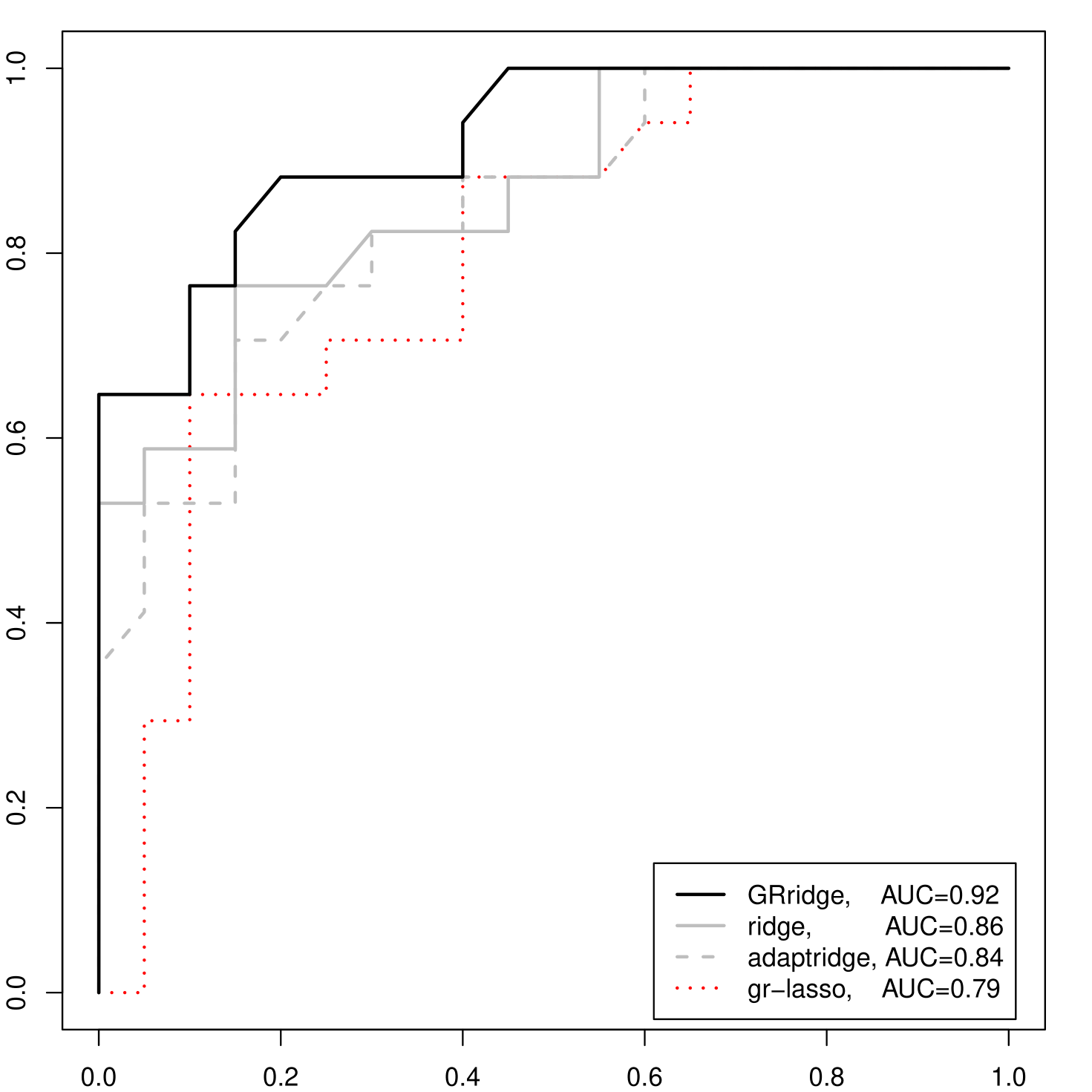
To assess whether the group-regularized ridge improves classification with respect to ordinary ridge, we computed ROC curves obtained by 10-fold cross-validation. Here, we compare with ridge regression on standardized covariates, because the latter was superior to the unstandardized version, as demonstrated above. In addition, we compare with the group lasso Meier et al. (2008), as implemented in the R package grpreg, using the same annotation-based groups as for GRridge. The last competitor is the adaptive ridge, as discussed above. Also these two methods are applied to the standardized covariates (which were verified to be superior to their unstandardized counterparts). Group lasso selected only the SSe group, but, surprisingly, not the CpG group.

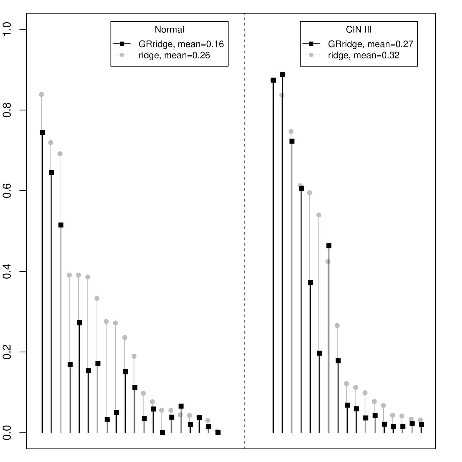
The resulting ROC curves depict the False Positive Rate (FPR) versus the True Positive Rate (FPR) for a dynamic cut-off for the predicted probability on CIN3. Figure 1(a) shows the results. We clearly observe superior performance of GRridge, with AUC = 0.92 (and 0.86, 0.84, 0.79 for ordinary ridge, adaptive ridge and group lasso, respectively). With respect to ordinary ridge, predictions improved for 33 out of 37 observations, as displayed in Figure 1(b). Note that adding the annotation-based groups to the variance-based groups improved the AUC only slightly, from 0.91 to 0.92, probably because AUC is a rank-based criterion. In fact, the predictions did improve for 32 out of 37 observations, leading to a relatively larger improvement (decrease) for the mean Brier residual, from 0.143 to 0.116.

In principle, we could use the results of the group-regularized ridge regression fitted on the first study, as presented in the previous section. However, the effect of the (possible) contamination may vary considerably across probes. For example, the differential signal of probes with hypo-methylation (affected $<$ normal) in the first study is diluted more than that of hyper-methylated probes. This can be illustrated in a simple deterministic setting. In case of hypo-methylation, consider a true ratio affected/normal = 0.4/0.8 = 1/2. Assume a contamination of 50%, then the measured ratio will be (0.4/2 + 0.8/2)/0.8 = 3/4, hence the ratio is 50% too large. Using the same numbers for hyper-methylation renders a measured ratio that is only 33% too small. In addition, it is well-known that ridge regression distributes differential signal over parameters corresponding to correlated probes. Hence, the magnitude of a particular coefficient also depends on other probes. Since the dilution in Study 2 affects probes differently, the applicability of Study 1 ridge regression results for analyzing Study 2 may be limited.

Therefore, we propose to use group penalties $\lambda_{g}$ that are simply based on $t$-test $p$-values as obtained by applying limma Smyth (2004) on Study 1. These $p$-values are then used to define a ranking-based partition with 100 groups of probes of minimal size $s=10$ (size gradually increasing with the $p$-value) as described above. To stabilize the estimates of $\lambda_{g}$ weights $\hat{\tau}^{2}_{g}\propto 1/\lambda_{g}$ for Study 2 are forced to be monotonously decreasing with increasing Study 1 $p$-values as described above. The function pava of the R library Iso is used for this purpose, which is illustrated in Supplementary Figure 2. In this setting, it is reasonable to precede our method by a mild prior filtering: only include those probes with $\text{FDR}\leq 0.5$ and a mean absolute difference larger than 0.1 (on log-scale) in Study 1. Then, our method applies group-specific regularization to the 9491 probes surviving these thresholds.

Given the earlier argument about a stronger dilution effect on hypo- than on hyper-methylated probes (as detected in Study 1), we also considered a second sign-based partition that distinguishes those two groups of probes. Finally, we added the variance-based and annotation-based partitions introduced in the first example. This illustrates the ability of our method to operate on multiple partitions. For this example, the adaptive group-regularized ridge used 3 re-penalization iterations. The CVL increased from -28.91 to -27.54, hence a 5% improvement. The sign-based and variance-based partitions had no effect on the results (hence rendering group-specific penalties equal to 1) on top of the $p$-value-based partition, illustrating the adaptive nature of the algorithm. The partition based on external $p$-values produced 100 group-specific penalties ranging from $1.3*10^{-3}$ to $13.3$ for $g=1,\ldots,100$, so indeed a large range (see also Supplementary Figure 3), illustrating the relevance of this partition. The annotation-based partition rendered $\lambda^{\prime}_{\text{CpG}}=0.17$, and much larger penalty multipliers for the other 5 classes. So, also for this data set the probes on the CpG-islands correspond to smaller penalties, which is biologically plausible.

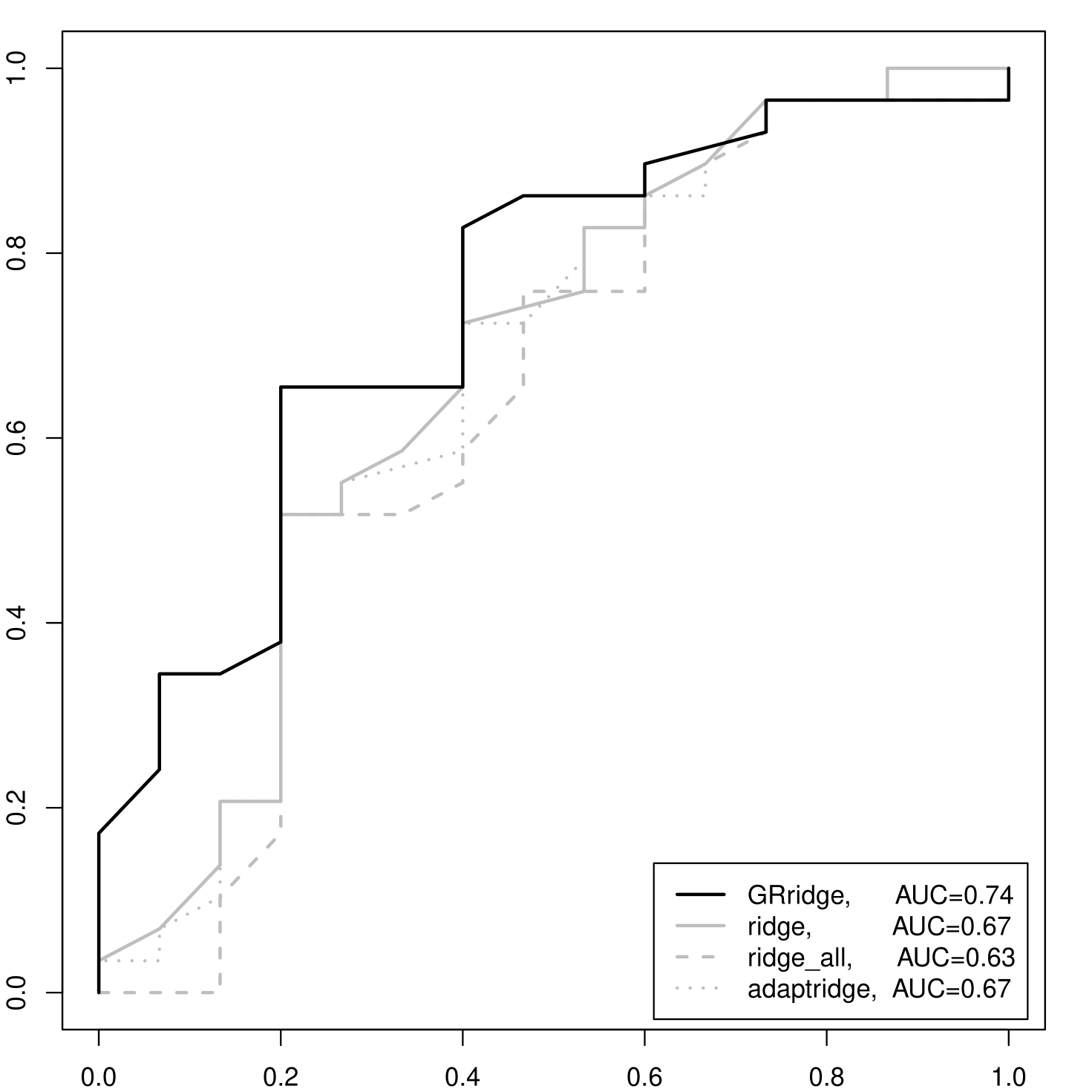
We compared GRridge with: i) ordinary ridge; ii) adaptive ridge; iii) group lasso with the same 100 $p$-value based groups (all three also applied to the filtered probe set); and iv) ordinary ridge on the entire, non-filtered probe set. For this data set, the group lasso did not select any group. Hence, no variable was selected either, rendering inferior prediction results. Probably, the weak differential signal per variable in this challenging data set caused the absence of selections for the group lasso. The ROC curves for the other three methods were obtained by applying leave-one-out cross-validation (LOOCV). Figure 2(a) shows the results: GRridge has a markedly higher AUC (0.74) than the ones corresponding to i) 0.67, ii) 0.67 and iv) 0.63.

We also checked whether the order in which the four partitions are used within each re-penalization iteration matters for the results. The final CVLs for all 24 possible orderings show very little variation: the range is $[-24.58,-24.54]$. Hence, we conclude that the sensitivity of the performance with respect to the ordering is very small for this data set.

References

- Amaratunga et al. (2008) Amaratunga, D. et al. (2008). Enriched random forests. Bioinformatics, 24, 2010–2014.
- Bergersen et al. (2011) Bergersen, L.C. et al. (2011). Weighted lasso with data integration. Stat. Appl. Genet. Mol. Biol., 10.
- Carvalho et al. (2009) Carvalho, C. et al. (2009). Handling sparsity via the horseshoe. J. Mach. Learn. Res., W&CP, pages 73–80.
- Cule et al. (2011) Cule, E. et al. (2011). Significance testing in ridge regression for genetic data. BMC Bioinf., 12, 372.
- Doksum et al. (2008) Doksum, K. et al. (2008). Nonparametric variable selection: the EARTH algorithm. J. Amer. Statist. Assoc., 103, 1609–1620.
- Farkas et al. (2013) Farkas, S. et al. (2013). Genome-wide DNA methylation assay reveals novel candidate biomarker genes in cervical cancer. Epigenetics, 8, 1213–1225.
- Futreal et al. (2004) Futreal, P. et al. (2004). A census of human cancer genes. Nat. Rev. Cancer, 4, 177–183.
- Goeman (2010) Goeman, J. (2010). L1 penalized estimation in the Cox proportional hazards model. Biom. J., 52, 70–84.
- Gok et al. (2010) Gok, M. et al. (2010). HPV testing on self collected cervicovaginal lavage specimens as screening method for women who do not attend cervical screening: cohort study. BMJ, 340, c1040.
- Gruber (1998) Gruber, M. (1998). Improving Efficiency by Shrinkage: The James–Stein and Ridge Regression Estimators. Statistics: A Series of Textbooks and Monographs.
- Hastie et al. (2008) Hastie, T. et al. (2008). The elements of statistical learning, 2nd ed. Springer, New York.
- Hoerl and Kennard (1970) Hoerl, A.E. and Kennard, R.W. (1970). Ridge regression: Biased estimation for nonorthogonal problems. Technometrics, 12, 55–67.
- Laird (2003) Laird, P. (2003). The power and the promise of DNA methylation markers. Nat. Rev. Cancer, 3, 253–266.
- le Cessie and van Houwelingen (1992) le Cessie, S. and van Houwelingen, J. (1992). Ridge estimators in logistic regression. Applied Statistics, 41, 191–201.
- Meier et al. (2008) Meier, L. et al. (2008). The group Lasso for logistic regression. J. R. Stat. Soc. Ser. B Stat. Methodol., 70, 53–71.
- Meijer and Goeman (2013) Meijer, R. and Goeman, J. (2013). Efficient approximate k-fold and leave-one-out cross-validation for ridge regression. Biom. J., 55, 141–155.
- Neuenschwander et al. (2010) Neuenschwander, B. et al. (2010). Summarizing historical information on controls in clinical trials. Clin. Trials, 7, 5–18.
- Park and Casella (2008) Park, T. and Casella, G. (2008). The Bayesian lasso. J. Amer. Statist. Assoc., 103, 681–686.
- Robertson et al. (1982) Robertson, T. et al. (1982). Order Restricted Statistical Inference. Wiley, New York.
- Smyth (2004) Smyth, G.K. (2004). Linear models and empirical Bayes methods for assessing differential expression in microarray experiments. Stat. Appl. Genet. Mol. Biol., 3, Art. 3.
- Tai and Pan (2007) Tai, F. and Pan, W. (2007). Incorporating prior knowledge of predictors into penalized classifiers with multiple penalty terms. Bioinformatics, 23, 1775–1782.
- Zou (2006) Zou, H. (2006). The adaptive lasso and its oracle properties. J. Amer. Statist. Assoc., 101, 1418–1429.
- Zwiener et al. (2014) Zwiener, I. et al. (2014). Transforming RNA-Seq data to improve the performance of prognostic gene signatures. PLoS ONE, 9, e85150.