Beyond ELBOs: A Large-Scale Evaluation of Variational Methods for Sampling
Abstract
Monte Carlo methods, Variational Inference, and their combinations play a pivotal role in sampling from intractable probability distributions. However, current studies lack a unified evaluation framework, relying on disparate performance measures and limited method comparisons across diverse tasks, complicating the assessment of progress and hindering the decision-making of practitioners. In response to these challenges, our work introduces a benchmark that evaluates sampling methods using a standardized task suite and a broad range of performance criteria. Moreover, we study existing metrics for quantifying mode collapse and introduce novel metrics for this purpose. Our findings provide insights into strengths and weaknesses of existing sampling methods, serving as a valuable reference for future developments. The code is publicly available here.
1 Introduction
Sampling methods are designed to address the challenge of generating approximate samples or estimating the intractable normalization constant for a probability density on of the form
| (1) |
where can be pointwise evaluated. This formulation has broad applications in fields such as Bayesian statistics and the natural sciences (Liu & Liu, 2001; Stoltz et al., 2010; Frenkel & Smit, 2023; Mittal et al., 2023).
Monte Carlo (MC) methods (Hammersley, 2013), including Annealed Importance Sampling (AIS) (Neal, 2001) and its Sequential Monte Carlo (SMC) extensions (Del Moral et al., 2006), have traditionally been considered the gold standard for addressing the sampling problem. An alternative approach is Variational Inference (VI) (Blei et al., 2017), where a tractable family of distributions is parameterized, and optimization tools are employed to maximize similarity to the intractable target distribution .
In recent years, there has been a surge of interest in the development of sampling methods that merge MC with VI techniques to approximate complex, potentially multimodal distributions (Wu et al., 2020a; Zhang & Chen, 2021; Arbel et al., 2021; Matthews et al., 2022; Jankowiak & Phan, 2022; Midgley et al., 2022; Berner et al., 2022; Richter et al., 2023; Vargas et al., 2023a, b; Akhound-Sadegh et al., 2024).
However, the evaluation of these methods faces significant challenges, including the absence of a standardized set of tasks and diverse performance criteria. This diversity complicates meaningful comparisons between methods. Existing evaluation protocols, such as the evidence lower bound (ELBO), often rely on samples from the model, restricting their evaluation capabilities to the model’s support. This limitation becomes especially problematic when assessing the ability to mitigate mode collapse on target densities with well-separated modes. To overcome this challenge, others propose the use of integral probability metrics (IPMs), like maximum mean discrepancy (Arenz et al., 2018) or Wasserstein distance (Richter et al., 2023; Vargas et al., 2023a), leveraging samples from the target density to assess performance beyond the model’s support. However, these metrics often involve subjective design choices such as kernel selection or cost function determination, potentially leading to biased evaluation protocols.
To address these challenges, our work introduces a comprehensive set of tasks for evaluating variational methods for sampling. We explore existing evaluation criteria and propose a novel metric specifically tailored to quantify mode collapse. Through this evaluation, we aim to provide valuable insights into the strengths and weaknesses of current sampling methods, contributing to the future design of more effective techniques and the establishment of standardized evaluation protocols.
2 Preliminaries
We provide an overview of Monte Carlo methods, Variational Inference, and combinations. The notation introduced in this section is used throughout the remainder of this work.
Monte Carlo Methods. A variety of Monte Carlo (MC) techniques have been developed to tackle the sampling problem and estimation of . In particular sequential importance sampling methods such as Annealed Importance Sampling (AIS) (Neal, 2001) and its Sequential Monte Carlo (SMC) extensions (Del Moral et al., 2006) are often regarded as a gold standard to compute . These approaches construct a sequence of distributions that ‘anneal’ smoothly from a tractable proposal distribution to the target distribution . One typically uses the geometric average, that is, , with for . Approximate samples from are then obtained by starting from and running a sequence of Markov chain Monte Carlo (MCMC) transitions that target .
Variational Inference. Variational inference (VI) (Blei et al., 2017) is a popular alternative to MCMC and SMC where one considers a flexible family of easy-to-sample distributions whose parameters are optimized by minimizing the reverse Kullback–Leibler (KL) divergence, i.e.,
| (2) |
It is well known that minimizing the reverse KL is equivalent to maximizing the evidence lower bound (ELBO) and that with equality if and only if . Later, VI was extended to other variational objectives such as -divergences (Li & Turner, 2016; Midgley et al., 2022), log-variance loss (Richter et al., 2020), trajectory balance, (Malkin et al., 2022a) or general - divergences (Wan et al., 2020). Typical choices for include mean-field approximations (Wainwright & Jordan, 2008), mixture models (Arenz et al., 2022) or normalizing flows (Papamakarios et al., 2021). To construct more flexible variational distributions (Agakov & Barber, 2004) modeled as the marginal of a latent variable model, i.e. 111Agakov & Barber (2004) coined the term ‘augmentation’ for . We adopt the more established terminology and refer to as a latent variable.. As this marginal is typically intractable, is then learned by minimizing a discrepancy measure between and an extended target where is an auxiliary conditional distribution. Using the chain rule for the KL-divergence (Cover, 1999) one obtains an extended version of the ELBO, that is,
| (3) |
Although the extended ELBO is often referred to as ELBO, latent variables introduce additional looseness, i.e., with equality if . To compute expectations with respect to , one typically chooses tractable distributions and and performs a Monte Carlo estimate using ancestral sampling.
Variational Monte Carlo Methods. Over recent years, the idea of using extended distributions has been further explored (Wu et al., 2020b; Geffner & Domke, 2021; Thin et al., 2021; Zhang et al., 2021; Doucet et al., 2022b; Geffner & Domke, 2022). In particular, these ideas marry Monte Carlo with variational techniques by constructing the variational distribution and extended target as Markov chains, i.e., and with , and tractable . Common choices of transition kernels include Gaussian distributions (Doucet et al., 2022b; Geffner & Domke, 2022) or normalizing flow maps (Wu et al., 2020a; Arbel et al., 2021; Matthews et al., 2022) and can be optimized by e.g. maximization of the extended ELBO via stochastic gradient ascent. Recently, Vargas et al. (2023a); Zhang & Chen (2021); Vargas et al. (2023b, 2024); Richter et al. (2023); Berner et al. (2022) explored the limit of in which case the Markov chains converge to forward and backward time stochastic differential equations (SDEs) (Anderson, 1982; Song et al., 2020) inducing the path distributions and which can be thought of as continuous time analogous of and respectively. Zhang & Chen (2021); Berner et al. (2022); Richter et al. (2023); Vargas et al. (2024) leveraged the continuous-time perspective to establish connections with Schrödinger bridges (Léonard, 2013) and stochastic optimal control (Dai Pra, 1991), resulting in the development of novel sampling algorithms.
Performance Criteria. Several performance criteria have been proposed for evaluating sampling methods, notably, those comparing the density ratio between the target and model density and integral probability metrics (IPMs).
Density ratio-based criteria make use of the ratio between the (unnormalized) target density and the model . Due to the intractability of for methods that work with latent variables, the density ratio between the joint distributions of and is considered, i.e.,
| (4) |
respectively. Note that and are also referred to as (unnormalized) importance weights. Using this notation, we can recover commonly used metrics such as the reverse effective sample size (ESSr) or the ELBO, that is,
| (5) |
respectively. Here, ‘reverse’ is used to denote that expecations are computed with respect to . In addition, if the true normalization constant is known, an importance-weighted reverse estimate of is often employed to report the esimation bias, i.e., with
| (6) |
Please note that extended versions of these criteria are obtainable by replacing with the extended version and taking expectations under the joint distribution .
3 Quantifying Mode-Collapse
Quantifying the ability to avoid mode collapse is difficult as identifying all modes of the target density and determining whether a model captures them accurately is inherently challenging. In particular, methods that are optimized using the reverse KL divergence are forced to assign high probability to regions with non-negligible probability in the target distribution . This is referred to as mode-seeking behavior and can result in an overemphasis on a limited set of modes, leading to mode collapse. Consequently, performance criteria that use expectations under the model , such as ELBO, (reverse) ESS, or , are influenced by the mode-seeking nature of the reverse KL divergence, making them less sensitive to mode collapse.
Here, we aim to explore criteria that are sensitive to mode collapse such as density-ratio based ‘forward’ criteria, that leverage expectations under and integral probability metrics (IPMs). Furthermore, we introduce entropic mode coverage, a novel criterion that leverages prior knowledge about the target to heuristically quantify mode coverage.
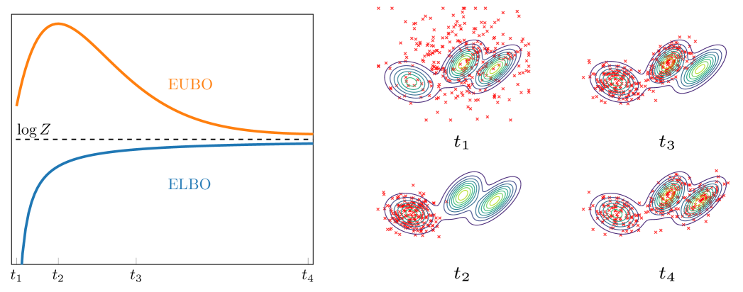
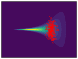
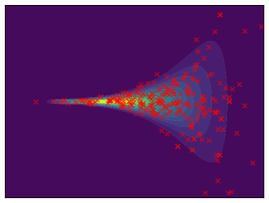
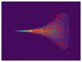
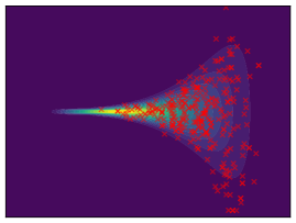
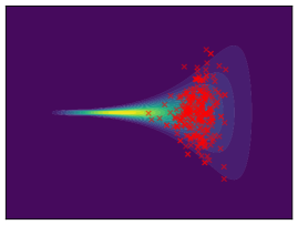
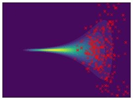
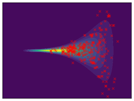
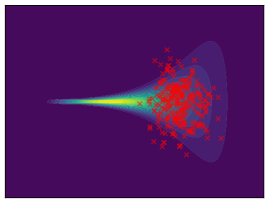
Forward Criteria. We discuss the ‘forward’ versions of the criteria discussed in Section 2. First, evidence upper bounds (EUBOs) are based on the forward KL divergence and have already been leveraged as learning objectives in VI (Ji & Shen, 2019). Here, we explore them as performance criteria that are sensitive to mode collapse. Formally, the EUBO is the sum of the forward KL and , that is,
| (7) |
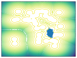
with importance weights . Due to the non-negativeness of the KL divergence, it is easy to see that with equality if and only if . Hence, a lower EUBO means that is closer to in a sense. The mass-covering nature of the forward KL leads to high EUBO values if the model fails to cover regions of non-negligible probability in the target distribution and is therefore well suited to quantify mode-collapse. This is further illustrated in Figure 1. We can again leverage the chain rule for the KL-divergence (Cover, 1999) to obtain an extended version of the EUBO, i.e., that satisfies , where the introduction of latent variables introduce additional looseness. The extended EUBO requires computing the importance weights and expectations under . The former depends on the specific choice of sampling algorithm and is further discussed in Section 4 when introducing the methods considered for evaluation. The latter can be approximated by propagating target samples back to using . Additionally, having access to samples from allows for computing forward versions of and ESS which have already been used to quantify mode collapse by e.g. (Midgley et al., 2023). Formally, they are defined as
| (8) |
where expectations are taken with respect to the target . For a detailed discussion see Appendix A.1.
Integral Probability Metrics. Alternatively, IPMs are often employed if samples from the target distribution are available (Arenz et al., 2018; Richter et al., 2023; Vargas et al., 2023a, 2024). Common IPMs for assessing sample quality are 2-Wasserstein distance () (Peyré et al., 2019) or the maximum mean discrepancy (MMD) (Gretton et al., 2012). The former uses a cost function to calculate the minimum cost required to transport probability mass from one distribution to another while the latter assesses distribution dissimilarity by examining the differences in their mean embeddings within a reproducing kernel Hilbert space (Aronszajn, 1950). For further details see Appendix A.2.
Entropic Mode Coverage. Inspired by inception scores and distances from generative modelling (Salimans et al., 2016; Heusel et al., 2017) we propose a heuristic approach for detecting mode collapse by introducing the entropic mode coverage (EMC). To compute EMC, we partition into disjoint subsets that describe different modes of the target density . Moreover, we introduce an auxiliary distribution that measures the probability of a sample being element of a mode descriptor, i.e., . We then compute the expected entropy of the auxiliary distribution, that is,
| (9) |
where the expectation is approximated using a Monte Carlo estimate. Here, denotes the number of samples drawn from . Please note that we employ the logarithm with a base of to ensure that . This choice of base facilitates a straightforward interpretation: A value of signifies a model that consistently produces samples that are elements of the same mode descriptor. In contrast, a value of represents a model that can produce samples from all mode descriptors with equal probability.
4 Benchmarking Methods
| Acronym | Method | Reference |
|---|---|---|
| MFVI | Gaussian Mean-Field VI | (Bishop, 2006) |
| GMMVI | Gaussian Mixture Model VI | (Arenz et al., 2022) |
| NFVI† | Normalizing Flow VI | (Rezende & Mohamed, 2015) |
| SMC | Sequential Monte Carlo | (Del Moral et al., 2006) |
| AFT | Annealed Flow Transport | (Arbel et al., 2021) |
| CRAFT | Continual Repeated AFT | (Matthews et al., 2022) |
| FAB | Flow Annealed IS Bootstrap | (Midgley et al., 2022) |
| ULA† | Uncorrected Langevin Annealing | (Thin et al., 2021) |
| MCD | Monte Carlo Diffusion | (Doucet et al., 2022a) |
| UHA† | Uncorrected Hamiltonian Annealing | (Geffner & Domke, 2021) |
| LDVI | Langevin Diffusion VI | (Geffner & Domke, 2022) |
| CMCD† | Controlled MCD | (Vargas et al., 2024) |
| PIS | Path Integral Sampler | (Zhang & Chen, 2021) |
| DIS | Time-Reversed Diffusion Sampler | (Berner et al., 2022) |
| DDS | Denoising Diffusion Sampler | (Vargas et al., 2023a) |
| GFN† | Generative Flow Networks | (Lahlou et al., 2023) |
| GBS | General Bridge Sampler | (Richter et al., 2023) |
| Funnel | Credit | Seeds | Cancer | Brownian | Ionosphere | Sonar | Digits | Fashion | LGCP | MoG | MoS | |
|---|---|---|---|---|---|---|---|---|---|---|---|---|
| True | ||||||||||||
| Samples from | ||||||||||||
| Mode descriptors | ||||||||||||
| Dimensionality | 10 | 25 | 26 | 31 | 32 | 35 | 61 | 196 | 784 | 1600 |
In this section, we elaborate on the methods included in this benchmark, categorizing them into three distinct groups based on the computation of importance weights. Please refer to Table 1 for an overview of these methods and to Appendix B for further details.
Tractable Density Models. Tractable density models allow for computing the model likelihood . It is therefore straightforward to compute performance criteria associated with importance weights . Notable works include factorized (‘mean-field’) Gaussian distributions (MFVI), Normalizing Flows (NFVI) (Rezende & Mohamed, 2015) and full rank Gaussian mixture models (GMMVI) (Arenz et al., 2022).
Sequential Importance Sampling Methods. Sequential importance sampling (SIS) methods define in terms of incremental importance sampling (IS) weights, that is, with
| (10) |
with annealed versions of . For example, choosing recovers AIS (Neal, 2001). Midgley et al. (2022) proposed to parameterize the proposal distribution with normalizing flows and, in combination with AIS, to minimize the -divergence, resulting in the Flow Annealed Importance Sampling Bootstrap (FAB) algorithm. Additionally, when AIS is coupled with resampling, it gives rise to Sequential Monte Carlo (SMC) as originally proposed by Del Moral et al. (2006).
Recent advancements include the development of Stochastic Normalizing Flows (Wu et al., 2020a), Annealed Flow Transport (AFT) (Arbel et al., 2021), and Continual Repeated AFT (CRAFT) (Matthews et al., 2022). These methods extend Sequential Monte Carlo by employing sets of normalizing flows that define deterministic transport maps between neighboring distributions . For further details on and the corresponding see Table 7. For an in-depth exploration of the commonalities and distinctions among these methods, please refer to (Matthews et al., 2022).
Diffusion-Based Methods. Diffusion-based methods typically build on stochastic differential equations (SDEs) with parameterized drift terms (Tzen & Raginsky, 2019), i.e.,
| (11) |
with diffusion coefficient and standard Brownian motion . Using the Euler-Maruyama method (Särkkä & Solin, 2019), their discretized counterparts can be characterized by Gaussian forward-backward transition kernels
| (12) |
with discretization step size . The extended (unnormalized) importance weights can then be constructed as
| (13) |
One line of work considers annealed Langevin dynamics to model Eq. (4). Works include Unadjusted Langevin Annealing (ULA) (Thin et al., 2021), Monte Carlo Diffusions (MCD) (Doucet et al., 2022a), Controlled Monte Carlo Diffusion (CMCD) (Vargas et al., 2024), Uncorrected Hamiltonian Annealing (UHA) (Geffner & Domke, 2021) and Langevin Diffusion Variational Inference (LDVI) (Geffner & Domke, 2022). A second line of work describes diffusion-based sampling from a stochastic optimal control perspective (Dai Pra, 1991). Works include methods such as Path Integral Sampler (PIS) (Zhang & Chen, 2021; Vargas et al., 2023b), Denoising Diffusion Sampler (DDS) (Vargas et al., 2023a), Time-Reversed Diffusion Sampler (DIS) (Berner et al., 2022) and Generative Flow Networks (GFN) (Lahlou et al., 2023; Malkin et al., 2022b; Zhang et al., 2023). Furthermore, Richter et al. (2023) identify several of these methods as special cases of a General Bridge Sampler (GBS) where both processes in Eq. 4 are freely parameterized. Specific choices of are detailed in Table 6. Lastly, we refer the interested reader to (Sendera et al., 2024) which concurrently benchmarked diffusion-based sampling methods.
![[Uncaptioned image]](https://cdn.awesomepapers.org/papers/e40e02c0-7869-467e-b96d-3a28473a446b/x2.png)
![[Uncaptioned image]](https://cdn.awesomepapers.org/papers/e40e02c0-7869-467e-b96d-3a28473a446b/x3.png)
5 Benchmarking Target Densities
| Funnel | MoS | MoG | |
|---|---|---|---|
 |
 |
 |
Here, we briefly summarize the target densities considered in this work. The dimensionality of the problem, if we have access to the log normalizer , target samples, or mode descriptors for computing the entropic mode coverage is presented in Table 2. Further details and formal definitions of the target densities can be found in Appendix C.
Bayesian Logistic Regression. We consider four experiments where we perform inference over the parameters of a Bayesian logistic regression model for binary classification. The datasets Credit and Cancer were taken from Nishihara et al. (2014). The former distinguishes individuals as either good or bad credit risks, while the latter deals with the classification of recurrence events in breast cancer. The Ionosphere dataset (Sigillito et al., 1989) involves classifying radar signals passing through the ionosphere as either good or bad. Similarly, the Sonar dataset (Gorman & Sejnowski, 1988) tackles the classification of sonar signals bounced off a metal cylinder versus those bounced off a roughly cylindrical rock.
Random Effect Regression. The Seeds data was collected by (Crowder, 1978). The goal is to perform inference over the variables of a random effect regression model that models the germination proportion of seeds arranged in a factorial layout by seed and type of root.
Time Series Models. We consider the Brownian time series model obtained by discretizing a stochastic differential equation, modeling a Brownian motion with a Gaussian observation model, developed by (Sountsov et al., 2020).
Spatial Statistics. The log Gaussian Cox process (LGCP) (Møller et al., 1998) is a probabilistic model commonly used in statistics to model spatial point patterns. In this work, the log Gaussian Cox process is applied to modeling the positions of pine saplings in Finland.
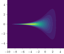
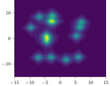
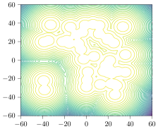
Synthetic Targets. We additionally consider synthetic target densities as they commonly give access to the true normalization constant , target samples, and mode descriptors. The Funnel target was introduced by (Neal, 2003) and provides a complex ‘funnel’-shaped distribution. Moreover, we consider two different types of mixture models: a mixture of isotropic Gaussians (MoG) as proposed by Midgley et al. (2022), and Student-t distributions (MoS). To obtain mode descriptors for a mixture model with components, i.e., we compute the density per component and say that if . Lastly, we follow Doucet et al. (2022a) and train NICE (Dinh et al., 2014) on a down-sampled variant of MNIST (Digits) (LeCun et al., 1998) and a variant of Fashion MNIST (Fashion) and use the trained model as target density. Here, we obtain the mode descriptors by training a classifier on samples from where the classes are represented by ten different digits. If we conclude .
6 Hyperparameters and Tuning
In this section, we provide details on hyperparameter tuning. For further information, please refer to Appendix D.
Tractable Density Methods. For MFVI, we used a batch size of 2000 and performed 100k gradient steps, tuning the learning rate via grid search. For targets with known support, we adjusted the initial model variance accordingly. For GMMVI, we adhered to the default settings from (Arenz et al., 2022), utilizing 100 samples per mixture component. We initialized with 10 components and employed an adaptive scheme to add and remove components heuristically. The initial variance of the components was set based on the target support, and we conducted 3000 training iterations.
Sequential Importance Sampling Methods. In SIS methods, we employed 2000 particles for training. All methods except FAB used 128 annealing steps; FAB followed the original 12 steps as proposed by its authors. The choice and parameters of the MCMC transition kernel significantly impacted performance. Hamilton-Monte Carlo (Duane et al., 1987) generally outperformed Metropolis-Hastings (Chib & Greenberg, 1995) (see Appendix F.3). Step sizes for and were tuned using grid search. For AFT and CRAFT, we used diagonal affine flows (Papamakarios et al., 2021), which yielded more robust results than complex flows like inverse autoregressive flows (Kingma et al., 2016) or neural spline flows (Durkan et al., 2019) (see Appendix F.6). FAB employed RealNVP (Dinh et al., 2016) for the proposal distribution . Learning rates for these flows were also tuned via grid search. For targets with known support, the variance of was set accordingly, otherwise, a grid search was performed. We used multinomial resampling with a threshold of 0.3 (Douc & Cappé, 2005).
Diffusion-based Methods. Training involved a batch size of 2000 and 40k gradient steps. SDEs were discretized with 128 steps, , and a fixed . The diffusion coefficient was chosen as , following (Vargas et al., 2023a) for better performance compared to linear or constant schedules. We used the architecture from (Zhang & Chen, 2021) with 2 layers of 64 hidden units each. For targets with known prior support, the initial model support was set accordingly. For all methods except PIS, this involved setting the variance of the prior distribution . For PIS, was carefully chosen. In MCD and LDVI, we learned the annealing schedule and end-to-end by maximizing the ELBO.
| Funnel | MoG | MoS | Digits | Fashion | ||||||
|---|---|---|---|---|---|---|---|---|---|---|
| MMD | MMD | MMD | MMD | MMD | ||||||
| MFVI | ||||||||||
| GMMVI | ||||||||||
| SMC | ||||||||||
| AFT | ||||||||||
| CRAFT | ||||||||||
| FAB | ||||||||||
| MCD | ||||||||||
| LDVI | N/A | N/A | ||||||||
| PIS | N/A | N/A | ||||||||
| DIS | ||||||||||
| DDS | ||||||||||
| GBS | ||||||||||
| MFVI | ||||||||||
| GMMVI | ||||||||||
| SMC | ||||||||||
| AFT | ||||||||||
| CRAFT | ||||||||||
| FAB | ||||||||||
| MCD | N/A | |||||||||
| LDVI | N/A | N/A | ||||||||
| PIS | ||||||||||
| DIS | ||||||||||
| DDS | ||||||||||
| GBS | ||||||||||
| ELBO | EUBO | ELBO | EUBO | ELBO | EUBO | ELBO | EUBO | ELBO | EUBO | |
| MFVI | ||||||||||
| GMMVI | ||||||||||
| SMC | ||||||||||
| AFT | ||||||||||
| CRAFT | ||||||||||
| FAB | ||||||||||
| MCD | N/A | |||||||||
| LDVI | N/A | N/A | ||||||||
| PIS | ||||||||||
| DIS | ||||||||||
| DDS | ||||||||||
| GBS | ||||||||||
7 Experiments
Here, we offer an overview of the evaluation protocol. Next, we present the results obtained for synthetic target densities, followed by those for real targets. We provide further results in Appendix E and ablation studies in Appendix F.
Evaluation Protocol. We compute all performance criteria 100 times during training, applying a running average with a length of 5 over these evaluations to obtain robust results within a single run. To ensure robustness across runs, we use four different random seeds and average the best results from each run. We use 2000 samples to compute the performance criteria and tune key hyperparameters such as the learning rate and variance of the initial proposal distribution . We report the EMC values corresponding to the method’s highest ELBO value to avoid high EMC values caused by a large initial support of the model.
![[Uncaptioned image]](https://cdn.awesomepapers.org/papers/e40e02c0-7869-467e-b96d-3a28473a446b/x7.png) |
![[Uncaptioned image]](https://cdn.awesomepapers.org/papers/e40e02c0-7869-467e-b96d-3a28473a446b/x8.png) |
![[Uncaptioned image]](https://cdn.awesomepapers.org/papers/e40e02c0-7869-467e-b96d-3a28473a446b/x9.png) |
![[Uncaptioned image]](https://cdn.awesomepapers.org/papers/e40e02c0-7869-467e-b96d-3a28473a446b/x10.png) |
![[Uncaptioned image]](https://cdn.awesomepapers.org/papers/e40e02c0-7869-467e-b96d-3a28473a446b/x11.png) |
![[Uncaptioned image]](https://cdn.awesomepapers.org/papers/e40e02c0-7869-467e-b96d-3a28473a446b/x12.png) |
|
| MFVI | GMMVI | MFVI | GMMVI | |||
![[Uncaptioned image]](https://cdn.awesomepapers.org/papers/e40e02c0-7869-467e-b96d-3a28473a446b/x13.png) |
![[Uncaptioned image]](https://cdn.awesomepapers.org/papers/e40e02c0-7869-467e-b96d-3a28473a446b/x14.png) |
![[Uncaptioned image]](https://cdn.awesomepapers.org/papers/e40e02c0-7869-467e-b96d-3a28473a446b/x15.png) |
![[Uncaptioned image]](https://cdn.awesomepapers.org/papers/e40e02c0-7869-467e-b96d-3a28473a446b/x16.png) |
![[Uncaptioned image]](https://cdn.awesomepapers.org/papers/e40e02c0-7869-467e-b96d-3a28473a446b/x17.png) |
![[Uncaptioned image]](https://cdn.awesomepapers.org/papers/e40e02c0-7869-467e-b96d-3a28473a446b/x18.png) |
|
| CRAFT | FAB | LDVI | GBS | FAB | LDVI |
| EMC | Digits | Fashion |
|---|---|---|
| MFVI | ||
| GMMVI | ||
| SMC | ||
| AFT | ||
| CRAFT | ||
| FAB | ||
| MCD | ||
| LDVI | ||
| PIS | ||
| DIS | ||
| DDS | ||
| GBS |
7.1 Evaluation on Synthetic Target Densities
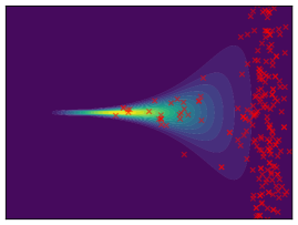
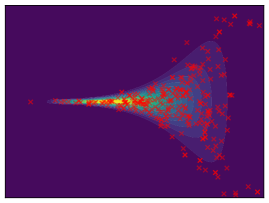
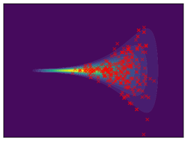
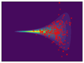
Funnel. We utilize the funnel distribution as a testing ground to assess whether sampling methods capture high curvatures in the target density. Our findings indicate that while most methods successfully capture the funnel-like structure, they struggle to generate samples at the neck and opening of the funnel, except for FAB and GMMVI (cf. Figure 4). This observation is further supported by quantitative analysis, revealing that both FAB and GMMVI achieve the best performance in terms of reverse and forward estimation of and evidence bounds as shown in Table 3.
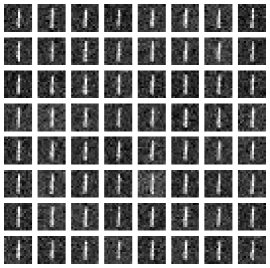
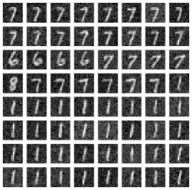
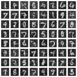
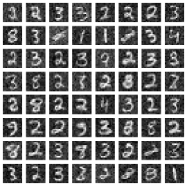
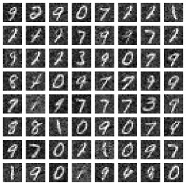
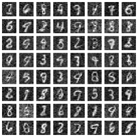
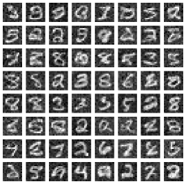
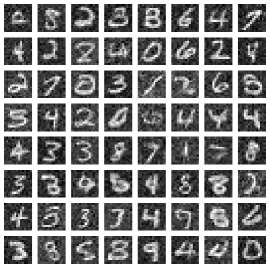
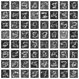
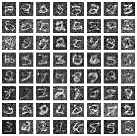
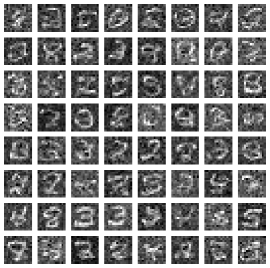
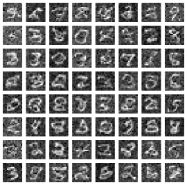
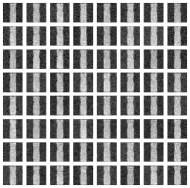
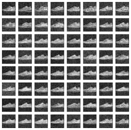
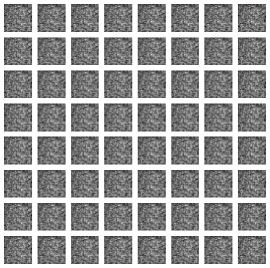
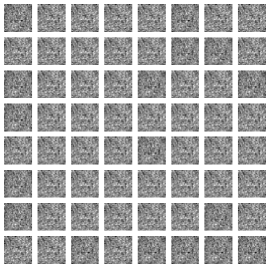
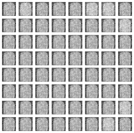
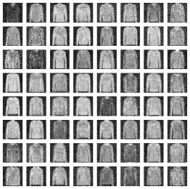
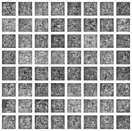
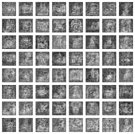
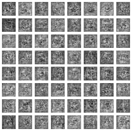
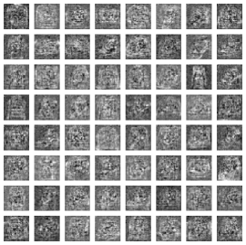
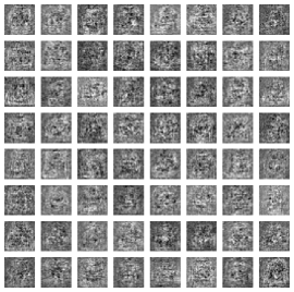
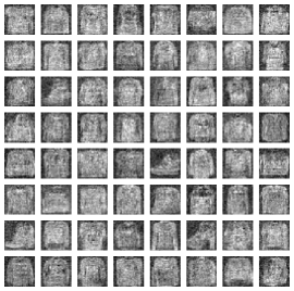
Digits and Fashion. For a comprehensive assessment of sampling methods, we conduct both qualitative and quantitative analyses on two high-dimensional target densities. For the qualitative analysis, model samples are interpreted as images and shown in Table 4. For the quantitative analysis, we report various performance criteria values, with results presented in Table 3. Additionally, we report EMC values in Table 4 to quantify mode collapse.
For Digits, most methods are able to find the majority of modes and produce high-quality samples, as visually evident from the sample visualizations and EMC values in Table 4. However, many methods, particularly diffusion-based ones, struggle to obtain reasonable estimations of . They also perform poorly in terms of lower and upper evidence bounds, as shown in Table 3. For Fashion, we observe that methods either suffer from mode collapse or produce low-quality samples. Interestingly, the methods experiencing mode collapse achieve the lowest estimation error of in both reverse and forward estimations.
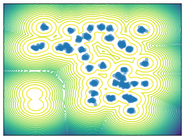
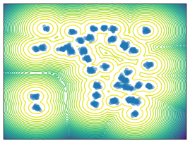
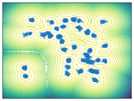
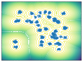
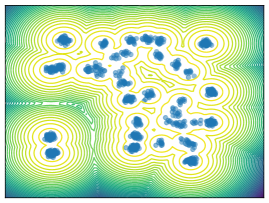
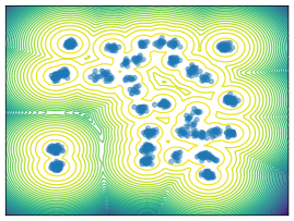
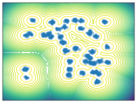
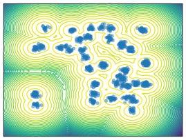
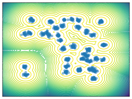
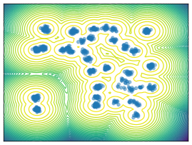
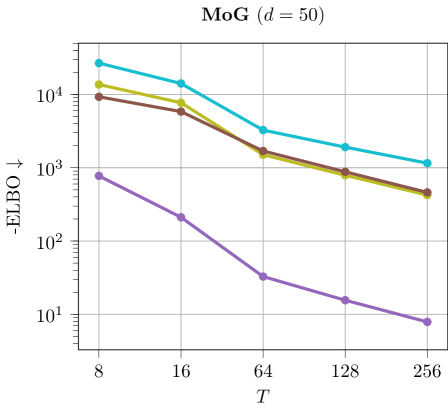
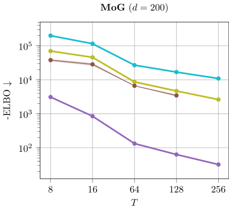
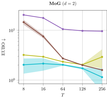
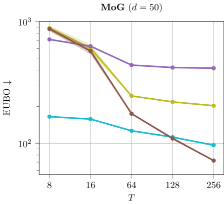
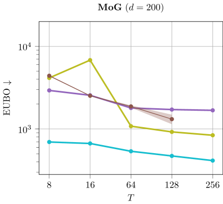
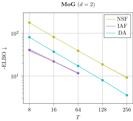
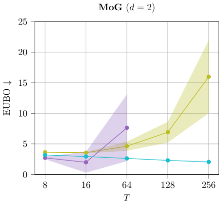
Mixture Models. We employ MoG and MoS to investigate mode collapse across different dimensions, specifically considering . For , all methods except MFVI demonstrate the capability to generate samples from all modes, as indicated by . This is further supported by visualizations in Figure 2. According to EMC, all methods except diffusion-based ones exhibit mode collapse for and .
7.2 Evaluation on Real Target Densities
For real-world target densities, we do not have access to the ground truth normalizer or samples from . Consequently, we present the ELBO values in Table 5. Surprisingly, we find that GMMVI performs well across all tasks, often outperforming more complex variational Monte Carlo methods. However, it is noteworthy that GMMVI encounters scalability challenges in very high-dimensional problems, such as LGCP. Another method, FAB, consistently performs well across a majority of tasks.
| ELBO | Credit | Seeds | Cancer | Brownian | Ionosphere | Sonar | LGCP |
|---|---|---|---|---|---|---|---|
| MFVI | |||||||
| GMMVI | OOM | ||||||
| SMC | |||||||
| AFT | N/A | ||||||
| CRAFT | |||||||
| FAB | |||||||
| MCD | N/A | N/A | |||||
| LDVI | N/A | N/A | |||||
| PIS | N/A | ||||||
| DDS | N/A | ||||||
| GBS | N/A | N/A |
8 Discussion and Conclusion
Here, we list several general observations O1)-O6) and observations tied to specific methods M1)-M6) that are based on the experiments from Section 7 and Appendix E and the Ablation studies in Appendix F.
O1) Mode collapse gets worse in high dimensions. We observe that several methods, that do not suffer from mode collapse in low-dimensional problems encounter significant mode collapse when applied to higher-dimensional ones (cf. Fig 2).
O2) ELBO and reverse estimates are not well suited for evaluating a model’s capability to avoid mode collapse. This observation is evident, for instance, in Table 4, where MFVI achieves relatively good ELBO and estimates despite suffering from mode collapse.
O3) While the EUBO helps to quantify mode collapse, comparing different method categories is challenging due to the additional looseness introduced by latent variables in the extended EUBO. This is evident on the Fashion dataset, where MFVI and GMMVI achieve a lower EUBO compared to most other methods, despite suffering from mode collapse.
O4) Despite being influenced by subjective design choices like the kernel or cost function, the 2-Wasserstein distance and Maximum Mean Discrepancy (MMD) generally show consistent performance across different sampling methods, as demonstrated in Table 3. Additionally, the quantitative results frequently align with the qualitative outcomes. For instance, this alignment is evident from GMMVI samples on Funnel or the GBS samples on the Fashion.
O5) For multimodal target distributions, both forward and reverse ESS tend to exhibit a ’binary’ pattern, frequently taking values of 0 or 1. Forward ESS, in particular, often tends to be predominantly zero for higher dimensional problems, further complicating the evaluation of mode collapse severity. In contrast, EUBO and ELBO offer a more continuous and informative perspective in assessing model performance (cf. Appendix E, Table 9).
O6) No single method exhibits superiority across all situations. Generally, GMMVI and FAB demonstrate good ELBO values across a diverse set of tasks, although both tend to suffer from mode collapse in high dimensions. In contrast, diffusion-based methods such as MCD and LDVI exhibit resilience against mode collapse but frequently fall short of achieving satisfactory ELBO values.
M1) Resampling causes mode collapse in high dimensions (cf. Ablation F.3). SIS methods, in particular, experience severe mode collapse in high dimensions, as illustrated in Figure 2. Notably, eliminating the resampling step in Sequential Monte Carlo (SMC) proves effective in mitigating this issue, but results in worse ELBO values.
M2) There exists an exploration-exploitation trade-off when setting the support of the proposal distribution in Variational Monte Carlo (cf. Ablation F.4). Opting for a small initial support of results in tight ELBO values but can limit coverage to only a few modes. Conversely, employing a sufficiently large initial support helps prevent mode collapse but introduces additional looseness in the ELBO.
M3) Learning the proposal distribution in Variational Monte Carlo methods often leads to mode collapse, especially in high dimensions. Training the base distribution end-to-end by maximizing the extended ELBO or pre-training the base distribution, for example, using methods like MFVI, results in mode collapse, as indicated in Ablation F.5 and Ablation F.8. Despite the occurrence of mode collapse, these strategies yield higher ELBOs, emphasizing the inherent exploration-exploitation trade-off discussed in M2).
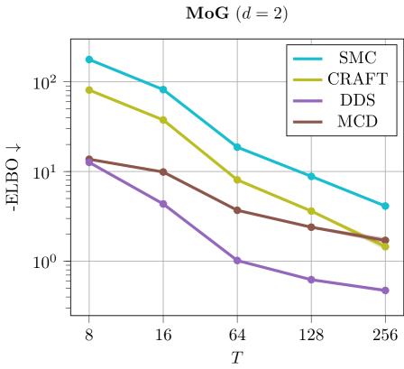
M4) Variational Monte Carlo methods heavily benefit from using a large number of steps . This is shown in Ablation F.2, where increasing the annealing steps for SIS methods and discretization steps for diffusion-based methods leads to tighter evidence bounds. However, increasing results in prolonged computational runtimes and demands substantial memory resources.
M5) GMMVI exhibits high sample efficiency (cf. Table 10). Arenz et al. (2022) employ a replay buffer to enhance the sample efficiency of GMMVI, leading to orders of magnitude fewer target evaluations required for convergence. Consequently, GMMVI may be the preferable choice when target evaluations are time-consuming.
M6) Langevin diffusion methods demonstrate low sample efficiency, as highlighted in Table 10. These methods require evaluating the target at each intermediate discretization step due to the score function being part of the SDE, and they typically need many iterations to converge. Other diffusion-based methods that do not require target evaluations at every step, such as DDS, often perform poorly and suffer from mode collapse (cf. Ablation F.7). To address this, Zhang & Chen (2021) proposed incorporating the score function into the network architecture, resulting again in poor sample efficiency.
9 Conclusion
In this work, we assessed the latest sampling methods using a standardized set of tasks. Our exploration encompassed various performance criteria, with a specific focus on quantifying mode collapse. Through a comprehensive evaluation, we illuminated the strengths and weaknesses of state-of-the-art sampling methods, thereby offering a valuable reference for future developments.
Impact Statement
This paper presents work whose goal is to advance the field of Machine Learning. There are many potential societal consequences of our work, none of which we feel must be specifically highlighted here.
Acknowledgments and Disclosure of Funding
We thank Julius Berner, Lorenz Richter, and Vincent Stimper for many useful discussions. D.B. acknowledges support by funding from the pilot program Core Informatics of the Helmholtz Association (HGF) and the state of Baden-Württemberg through bwHPC, as well as the HoreKa supercomputer funded by the Ministry of Science, Research and the Arts Baden-Württemberg and by the German Federal Ministry of Education and Research.
References
- Agakov & Barber (2004) Agakov, F. V. and Barber, D. An auxiliary variational method. In Advances in Neural Information Processing Systems, 2004.
- Akhound-Sadegh et al. (2024) Akhound-Sadegh, T., Rector-Brooks, J., Bose, A. J., Mittal, S., Lemos, P., Liu, C.-H., Sendera, M., Ravanbakhsh, S., Gidel, G., Bengio, Y., et al. Iterated denoising energy matching for sampling from boltzmann densities. arXiv preprint arXiv:2402.06121, 2024.
- Anderson (1982) Anderson, B. D. Reverse-time diffusion equation models. Stochastic Processes and their Applications, 12(3):313–326, 1982.
- Arbel et al. (2021) Arbel, M., Matthews, A., and Doucet, A. Annealed flow transport monte carlo. In International Conference on Machine Learning, pp. 318–330. PMLR, 2021.
- Arenz et al. (2018) Arenz, O., Neumann, G., and Zhong, M. Efficient gradient-free variational inference using policy search. In International conference on machine learning, pp. 234–243. PMLR, 2018.
- Arenz et al. (2022) Arenz, O., Dahlinger, P., Ye, Z., Volpp, M., and Neumann, G. A unified perspective on natural gradient variational inference with gaussian mixture models. arXiv preprint arXiv:2209.11533, 2022.
- Aronszajn (1950) Aronszajn, N. Theory of reproducing kernels. Transactions of the American mathematical society, 68(3):337–404, 1950.
- Berner et al. (2022) Berner, J., Richter, L., and Ullrich, K. An optimal control perspective on diffusion-based generative modeling. arXiv preprint arXiv:2211.01364, 2022.
- Bishop (2006) Bishop, C. Pattern recognition and machine learning. Springer google schola, 2:531–537, 2006.
- Blei et al. (2017) Blei, D. M., Kucukelbir, A., and McAuliffe, J. D. Variational inference: A review for statisticians. Journal of the American statistical Association, 112(518):859–877, 2017.
- Chib & Greenberg (1995) Chib, S. and Greenberg, E. Understanding the metropolis-hastings algorithm. The american statistician, 49(4):327–335, 1995.
- Cover (1999) Cover, T. M. Elements of information theory. John Wiley & Sons, 1999.
- Crowder (1978) Crowder, M. J. Beta-binomial anova for proportions. Applied statistics, pp. 34–37, 1978.
- Dai Pra (1991) Dai Pra, P. A stochastic control approach to reciprocal diffusion processes. Applied mathematics and Optimization, 23(1):313–329, 1991.
- Del Moral et al. (2006) Del Moral, P., Doucet, A., and Jasra, A. Sequential Monte Carlo samplers. Journal of the Royal Statistical Society: Series B (Statistical Methodology), 68(3):411–436, 2006.
- Dinh et al. (2014) Dinh, L., Krueger, D., and Bengio, Y. Nice: Non-linear independent components estimation. arXiv preprint arXiv:1410.8516, 2014.
- Dinh et al. (2016) Dinh, L., Sohl-Dickstein, J., and Bengio, S. Density estimation using real nvp. arXiv preprint arXiv:1605.08803, 2016.
- Douc & Cappé (2005) Douc, R. and Cappé, O. Comparison of resampling schemes for particle filtering. In ISPA 2005. Proceedings of the 4th International Symposium on Image and Signal Processing and Analysis, 2005., pp. 64–69. Ieee, 2005.
- Doucet et al. (2022a) Doucet, A., Grathwohl, W., Matthews, A. G., and Strathmann, H. Score-based diffusion meets annealed importance sampling. Advances in Neural Information Processing Systems, 35:21482–21494, 2022a.
- Doucet et al. (2022b) Doucet, A., Grathwohl, W., Matthews, A. G. d. G., and Strathmann, H. Score-based diffusion meets annealed importance sampling. In Advances in Neural Information Processing Systems, 2022b.
- Duane et al. (1987) Duane, S., Kennedy, A. D., Pendleton, B. J., and Roweth, D. Hybrid monte carlo. Physics letters B, 195(2):216–222, 1987.
- Durkan et al. (2019) Durkan, C., Bekasov, A., Murray, I., and Papamakarios, G. Neural spline flows. Advances in neural information processing systems, 32, 2019.
- Frenkel & Smit (2023) Frenkel, D. and Smit, B. Understanding molecular simulation: from algorithms to applications. Elsevier, 2023.
- Geffner & Domke (2021) Geffner, T. and Domke, J. MCMC variational inference via uncorrected Hamiltonian annealing. In Advances in Neural Information Processing Systems, 2021.
- Geffner & Domke (2022) Geffner, T. and Domke, J. Langevin diffusion variational inference. arXiv preprint arXiv:2208.07743, 2022.
- Gorman & Sejnowski (1988) Gorman, R. P. and Sejnowski, T. J. Analysis of hidden units in a layered network trained to classify sonar targets. Neural networks, 1(1):75–89, 1988.
- Gretton et al. (2012) Gretton, A., Borgwardt, K. M., Rasch, M. J., Schölkopf, B., and Smola, A. A kernel two-sample test. The Journal of Machine Learning Research, 13(1):723–773, 2012.
- Hammersley (2013) Hammersley, J. Monte carlo methods. Springer Science & Business Media, 2013.
- Heusel et al. (2017) Heusel, M., Ramsauer, H., Unterthiner, T., Nessler, B., and Hochreiter, S. Gans trained by a two time-scale update rule converge to a local nash equilibrium. Advances in neural information processing systems, 30, 2017.
- Jankowiak & Phan (2022) Jankowiak, M. and Phan, D. Surrogate likelihoods for variational annealed importance sampling. In International Conference on Machine Learning, pp. 9881–9901. PMLR, 2022.
- Ji & Shen (2019) Ji, C. and Shen, H. Stochastic variational inference via upper bound. arXiv preprint arXiv:1912.00650, 2019.
- Kingma & Ba (2014) Kingma, D. P. and Ba, J. Adam: A method for stochastic optimization. arXiv preprint arXiv:1412.6980, 2014.
- Kingma et al. (2016) Kingma, D. P., Salimans, T., Jozefowicz, R., Chen, X., Sutskever, I., and Welling, M. Improved variational inference with inverse autoregressive flow. Advances in neural information processing systems, 29, 2016.
- Lahlou et al. (2023) Lahlou, S., Deleu, T., Lemos, P., Zhang, D., Volokhova, A., Hernández-Garcıa, A., Ezzine, L. N., Bengio, Y., and Malkin, N. A theory of continuous generative flow networks. In International Conference on Machine Learning, pp. 18269–18300. PMLR, 2023.
- LeCun et al. (1998) LeCun, Y., Bottou, L., Bengio, Y., and Haffner, P. Gradient-based learning applied to document recognition. Proceedings of the IEEE, pp. 2278–2324, 1998. doi: 10.1109/5.726791.
- Léonard (2013) Léonard, C. A survey of the schr” odinger problem and some of its connections with optimal transport. arXiv preprint arXiv:1308.0215, 2013.
- Li & Turner (2016) Li, Y. and Turner, R. E. Rényi divergence variational inference. Advances in neural information processing systems, 29, 2016.
- Liu & Liu (2001) Liu, J. S. and Liu, J. S. Monte Carlo strategies in scientific computing, volume 75. Springer, 2001.
- Malkin et al. (2022a) Malkin, N., Jain, M., Bengio, E., Sun, C., and Bengio, Y. Trajectory balance: Improved credit assignment in gflownets. Advances in Neural Information Processing Systems, 35:5955–5967, 2022a.
- Malkin et al. (2022b) Malkin, N., Lahlou, S., Deleu, T., Ji, X., Hu, E., Everett, K., Zhang, D., and Bengio, Y. Gflownets and variational inference. arXiv preprint arXiv:2210.00580, 2022b.
- Matthews et al. (2022) Matthews, A., Arbel, M., Rezende, D. J., and Doucet, A. Continual repeated annealed flow transport monte carlo. In International Conference on Machine Learning, pp. 15196–15219. PMLR, 2022.
- Midgley et al. (2022) Midgley, L. I., Stimper, V., Simm, G. N., Schölkopf, B., and Hernández-Lobato, J. M. Flow annealed importance sampling bootstrap. arXiv preprint arXiv:2208.01893, 2022.
- Midgley et al. (2023) Midgley, L. I., Stimper, V., Antorán, J., Mathieu, E., Schölkopf, B., and Hernández-Lobato, J. M. Se (3) equivariant augmented coupling flows. arXiv preprint arXiv:2308.10364, 2023.
- Mittal et al. (2023) Mittal, S., Bracher, N. L., Lajoie, G., Jaini, P., and Brubaker, M. A. Exploring exchangeable dataset amortization for bayesian posterior inference. In ICML 2023 Workshop on Structured Probabilistic Inference & Generative Modeling, 2023.
- Møller et al. (1998) Møller, J., Syversveen, A. R., and Waagepetersen, R. P. Log gaussian cox processes. Scandinavian journal of statistics, 25(3):451–482, 1998.
- Neal (2001) Neal, R. M. Annealed importance sampling. Statistics and Computing, 11(2):125–139, 2001.
- Neal (2003) Neal, R. M. Slice sampling. The annals of statistics, 31(3):705–767, 2003.
- Nishihara et al. (2014) Nishihara, R., Murray, I., and Adams, R. P. Parallel mcmc with generalized elliptical slice sampling. The Journal of Machine Learning Research, 15(1):2087–2112, 2014.
- Papamakarios et al. (2021) Papamakarios, G., Nalisnick, E., Rezende, D. J., Mohamed, S., and Lakshminarayanan, B. Normalizing flows for probabilistic modeling and inference. The Journal of Machine Learning Research, 22(1):2617–2680, 2021.
- Peyré et al. (2019) Peyré, G., Cuturi, M., et al. Computational optimal transport: With applications to data science. Foundations and Trends® in Machine Learning, 11(5-6):355–607, 2019.
- Rezende & Mohamed (2015) Rezende, D. and Mohamed, S. Variational inference with normalizing flows. In International conference on machine learning, pp. 1530–1538. PMLR, 2015.
- Richter et al. (2020) Richter, L., Boustati, A., Nüsken, N., Ruiz, F., and Akyildiz, O. D. Vargrad: a low-variance gradient estimator for variational inference. Advances in Neural Information Processing Systems, 33:13481–13492, 2020.
- Richter et al. (2023) Richter, L., Berner, J., and Liu, G.-H. Improved sampling via learned diffusions. arXiv preprint arXiv:2307.01198, 2023.
- Salimans et al. (2016) Salimans, T., Goodfellow, I., Zaremba, W., Cheung, V., Radford, A., and Chen, X. Improved techniques for training gans. Advances in neural information processing systems, 29, 2016.
- Särkkä & Solin (2019) Särkkä, S. and Solin, A. Applied stochastic differential equations, volume 10. Cambridge University Press, 2019.
- Sendera et al. (2024) Sendera, M., Kim, M., Mittal, S., Lemos, P., Scimeca, L., Rector-Brooks, J., Adam, A., Bengio, Y., and Malkin, N. On diffusion models for amortized inference: Benchmarking and improving stochastic control and sampling. arXiv preprint arXiv:2402.05098, 2024.
- Shapiro (2003) Shapiro, A. Monte carlo sampling methods. Handbooks in operations research and management science, 10:353–425, 2003.
- Sigillito et al. (1989) Sigillito, V. G., Wing, S. P., Hutton, L. V., and Baker, K. B. Classification of radar returns from the ionosphere using neural networks. Johns Hopkins APL Technical Digest, 10(3):262–266, 1989.
- Song et al. (2020) Song, Y., Sohl-Dickstein, J., Kingma, D. P., Kumar, A., Ermon, S., and Poole, B. Score-based generative modeling through stochastic differential equations. arXiv preprint arXiv:2011.13456, 2020.
- Sountsov et al. (2020) Sountsov, P., Radul, A., and contributors. Inference gym, 2020. URL https://pypi.org/project/inference_gym.
- Stoltz et al. (2010) Stoltz, G., Rousset, M., et al. Free energy computations: A mathematical perspective. World Scientific, 2010.
- Thin et al. (2021) Thin, A., Kotelevskii, N., Durmus, A., Moulines, E., Panov, M., and Doucet, A. Monte Carlo variational auto-encoders. In International Conference on Machine Learning, 2021.
- Tzen & Raginsky (2019) Tzen, B. and Raginsky, M. Neural stochastic differential equations: Deep latent gaussian models in the diffusion limit. arXiv preprint arXiv:1905.09883, 2019.
- Vargas et al. (2023a) Vargas, F., Grathwohl, W., and Doucet, A. Denoising diffusion samplers. arXiv preprint arXiv:2302.13834, 2023a.
- Vargas et al. (2023b) Vargas, F., Ovsianas, A., Fernandes, D., Girolami, M., Lawrence, N. D., and Nüsken, N. Bayesian learning via neural schrödinger–föllmer flows. Statistics and Computing, 33(1):3, 2023b.
- Vargas et al. (2024) Vargas, F., Padhy, S., Blessing, D., and Nüsken, N. Transport meets variational inference: Controlled monte carlo diffusions. In The Twelfth International Conference on Learning Representations, 2024.
- Wainwright & Jordan (2008) Wainwright, M. J. and Jordan, M. I. Graphical Models, Exponential Families, and Variational Inference. Foundations and Trends® in Machine Learning, 1(1–2):1–305, November 2008.
- Wan et al. (2020) Wan, N., Li, D., and Hovakimyan, N. F-divergence variational inference. Advances in neural information processing systems, 33:17370–17379, 2020.
- Wu et al. (2020a) Wu, H., Köhler, J., and Noé, F. Stochastic normalizing flows. Advances in Neural Information Processing Systems, 33:5933–5944, 2020a.
- Wu et al. (2020b) Wu, H., Köhler, J., and Noé, F. Stochastic normalizing flows. In Advances in Neural Information Processing Systems, 2020b.
- Zhang et al. (2023) Zhang, D., Chen, R. T. Q., Liu, C.-H., Courville, A., and Bengio, Y. Diffusion generative flow samplers: Improving learning signals through partial trajectory optimization. arXiv preprint arXiv:2310.02679, 2023.
- Zhang et al. (2021) Zhang, G., Hsu, K., Li, J., Finn, C., and Grosse, R. Differentiable annealed importance sampling and the perils of gradient noise. In Advances in Neural Information Processing Systems, 2021.
- Zhang & Chen (2021) Zhang, Q. and Chen, Y. Path integral sampler: a stochastic control approach for sampling. arXiv preprint arXiv:2111.15141, 2021.
Appendix A Performance Criteria Details
Here, we provide further details on the computation of the various performance criteria introduced in the main manuscript.
A.1 Density-Ratio-Based Criteria
Forward and Reverse Importance-Weighted Estimation of . Using the definition of the normalization constant, the importance-weighted reverse estimate of is given by
| (14) |
where denotes the number of samples from used for the Monte Carlo estimate of the expectation. Using the identity , we obtain the forward estimation of as
| (15) |
where denotes the number of samples from used for the Monte Carlo estimate of the expectation.
Forward and Reverse Effective Sample Size. The (reverse) effective sample size (ESS), or equivalently, reverse ESS (Shapiro, 2003) is defined as
| (16) |
where is approximated using the reverse estimate as defined in Eq. 14. Using the definition of the ESS, it is straightforward to see that
| (17) |
where is approximated using the forward estimate as defined in Eq. 15.
A.2 Integral Probability Metrics
Maximum Mean Discrepancy. The Maximum Mean Discrepancy (MMD) (Gretton et al., 2012) is a kernel-based measure of distance between two distributions. The MMD quantifies the dissimilarity between these distributions by comparing their mean embeddings in a reproducing kernel Hilbert space (RKHS) (Aronszajn, 1950) with kernel . In our setting, we are interested in computing the MMD between a model and target distribution . Formally, if is the RKHS associated with kernel function , the MMD between and is the integral probability metric defined by:
| (18) |
with and if and only if . The minimum variance unbiased estimate of between two sample sets and with sizes and respectively is given by
| (19) |
In our experiments, we took a squared exponential kernel given by , where the bandwidth is determined using the median heuristic (Gretton et al., 2012). The code for computing the MMD was built upon https://github.com/antoninschrab/mmdfuse-paper.
Entropic Optimal Transport Distance. The 2-Wasserstein distance is given by
| (20) |
with cost , chosen as in our experiments. To obtain a tractable objective, an entropy regularized version has been proposed (Peyré et al., 2019), that is,
| (21) |
with entropy . We chose for all experiments. The code was taken from https://github.com/ott-jax/ott.
A.3 Extending the Entropic Mode Coverage
If the true mode probabilities are not uniformly distributed, EMC=1 does not correspond to the optimal value. In that case, we propose the expected Jensen-Shannon divergence, that is,
| (22) |
with
| (23) |
as an alternative heuristic to quantify mode collapse. Similar to EMC, EJS is bounded and is straightforward to interpret: When employing the base 2 logarithm, EJS remains bounded, i.e., . Moreover implies that the model matches the potentially unbalanced true mode probabilities, while indicates that and possess no overlapping probability mass.
Appendix B Details on Unnormalized Importance Weights / Density Ratios
Here, we provide further details on how the unnormalized importance weights / density ratios are computed for different methods.
Tractable Density Methods. For models with tractable density the marginal (unnormalized) importance weights can trivially computed using
Diffusion-based Methods. For diffusion-based methods, the extended importance weights can then be constructed as
| (24) |
The different choices of forward and backward transition kernels are listed in Table 6. Some methods such as DDS (Vargas et al., 2023a), PIS (Zhang & Chen, 2021) and GFN (Zhang et al., 2023) introduce a reference process with
| (25) |
This allows for rewriting Eq. 24 as
| (26) |
potentially resulting in more tractable density ratios compared to Eq. 24. For concrete examples see e.g. (Zhang et al., 2023). A continuous-time analogous of the reference process is detailed in (Vargas et al., 2024). Moreover, in continuous-time, the importance weights correspond to a Radon–Nikodym derivative. For the sake of simplicity, we only consider the discrete-time setting in this work. We refer the reader to (Vargas et al., 2024; Richter et al., 2023) for further details.
| Method | |||
|---|---|---|---|
| DDS | |||
| DIS | |||
| PIS/GFN | |||
| ULA | arbitrary∗ | ||
| MCD | arbitrary∗ | ||
| CMCD | arbitrary∗ | ||
| GBS | arbitrary∗ |
Sequential Importance Sampling Methods. Sequential importance sampling methods express the importance weights in terms of incremental importance sampling weights, i.e.,
For given forward transitions , the optimal backward transitions ensure that . As the optimal transitions are typically not available, SMC uses the AIS approximation (Neal, 2001). Moreover flow transport methods (Wu et al., 2020a; Arbel et al., 2021; Matthews et al., 2022) use a flow as a deterministic map to approximate the incremental IS weights. In Table 7, we list different and their corresponding incremental importance sampling weights.
| Method | ||||
|---|---|---|---|---|
| Optimal | ||||
| AIS/SMC/FAB | ||||
| AFT/CRAFT |
Appendix C Benchmark Target Details
Here, we introduce the target densities considered in this benchmark more formally.
C.1 Bayesian Logistic Regression
We used four binary classification problems in our benchmark, which have also been used in various other work to compare different state-of-the-art methods in variational inference and Markov chain Monte Carlo. We assess the performance of a Bayesian logistic model with:
on two standardized datasets , namely Ionosphere () with 351 data points and Sonar () with 208 data points.
The German Credit dataset consists of () features and 1000 data points, while the Breast Cancer dataset has () dimensions with 569 data points, which we standardize and apply linear logistic regression.
C.2 Random Effect Regression
The Seeds () target is a random effect regression model trained on the seeds dataset:
The goal is to do inference over the variables and for , given observed values for and .
C.3 Time Series Models
The Brownian () model corresponds to the time discretization of a Brownian motion:
inference is performed over the variables and given the observations .
C.4 Spatial Statistics
The Log Gaussian Cox process () is a popular high-dimensional task in spatial statistics (Møller et al., 1998) which models the position of pine saplings. Using a grid, we obtain the unnormalized target density by
C.5 Synthetic Targets
We evaluate on three different mixture models which all follow the structure, that is,
where denotes the number of components.
The MoG () distribution, taken from (Midgley et al., 2022), consists of mixture components with
where refers to a uniform distribution on .
The MoS () comprises 10 Student’s t-distributions , where the refers to the degree of freedom. Generally, Student’s t-distributions have heavier tails compared to Gaussian distributions, making them sharper and more challenging to approximate.
where refers to the translation of the individual components.
The Funnel () target introduced in (Neal, 2003) is a challenging funnel-shaped distribution given by
with .
Appendix D Algorithms and Parameter Choices
Here, we discuss the parameter choices of all methods. Most of these choices are based on recommendations of the authors. For some choices, we run ablation studies to find suitable values.
Gaussian Mean Field Variational Inference (MFVI). We updated the mean and the diagonal covariance matrix using the Adam optimizer (Kingma & Ba, 2014) for iterations with a batch size of . We ensured non-negativeness of the variance by using a transformation. The mean is initialized at for all experiments. The initial covariance/scale and the learning rate are set according to Table 8.
Gaussian Mixture Model Variational Inference (GMMVI). For GMMVI, we ported the tensorflow implementation of https://github.com/OlegArenz/gmmvi to Jax and integrated it into our framework. We use the specifications (Arenz et al., 2022) described as SAMTRUX. We make use of their adaptive component initializer and start using ten components. The initial variance of the components is set according to Table 8.
Sequential Monte Carlo (SMC). For the Sequential Monte Carlo (SMC) approach, we leveraged the codebase available at https://github.com/google-deepmind/annealed_flow_transport. We used particles and annealing steps (temperatures) . We used resampling with a threshold of . We used one Hamiltonian Monte Carlo (HMC) step per temperature with leapfrog steps. We tuned the stepsize of HMC according to Table 8 where we used different stepsizes depending on the annealing parameter . We additionally tune the scale of the initial proposal distribution as shown in Table 8.
Continual Repeated Annealed Flow Transport (CRAFT/AFT). As AFT and CRAFT build on Sequential Monte Carlo (SMC), we employed the same SMC specifications detailed above. Notably, we found that employing simpler flows in conjunction with a greater number of temperatures yielded superior and more robust performance compared to the use of more sophisticated flows such as RealNVP or Neural Spline Flows. Consequently, we opted for 128 temperatures, utilizing diagonal affine flows as the transport map. Specifically for AFT, we determined that 400 iterations per temperature were sufficient to achieve converged training results. For CRAFT and SNF, we found that a total of 3000 iterations provided satisfactory convergence during training. For all methods, we use particles for training and testing and tune the learning rate and the scale of the initial proposal distribution as shown in Table 8.
Flow Annealed Importance Sampling Bootstrap (FAB). We built our implementation off of https://github.com/lollcat/fab-jax. We adjusted the parameters of FAB in accordance with the author’s most important hyperparameter suggestions and to ensure that SMC performs reasonably well. To achieve this, we set the number of temperatures to and used HMC as MCMC kernel. For the flow architecture we use RealNVP (Dinh et al., 2016) where the conditioner is given by an 8-layer MLP. Furthermore, we utilized FAB’s replay buffer to speed up computations. The learning rate and base distribution scale are adjusted for target specificity, following the specifications outlined in Table 8. We used a batch size of 2048 and trained FAB for 3000 iterations which proved sufficient for achieving a satisfactory convergence.
Denoising Diffusion Sampler (DDS) and Path Integral Sampler (PIS). We use the implementation of https://github.com/franciscovargas/denoising_diffusion_samplers to integrate the Diffusion and Path Integral Sampler into our framework. We set the parameters of the SDEs according to the authors, i.e., (Zhang & Chen, 2021) and (Vargas et al., 2023a) and use 128 timesteps and a batch size of 2000 if not otherwise stated. Both methods use the network proposed in (Zhang & Chen, 2021) which uses a sinusoidal position embedding for the timestep and uses the gradient of the log target density as an additional term. As proposed, we use a two-layer neural network with hidden units. For DDS we use a cosine scheduler (Vargas et al., 2023a) and for PIS a uniform time scheduler (Zhang & Chen, 2021). Both methods were trained using iterations.
Monte Carlo Diffusions (MCD) and Langevin Diffusion Variational Inference (LDVI). We build our implementation of Langevin Diffusion methods on https://github.com/tomsons22/LDVI. For experiments where performance is solely measured in terms of ELBO, due to the lack of samples from or access to , we train all parameters of the SDE by maximizing the EUBO as suggested by (Geffner & Domke, 2021). For multimodal target densities, we fix the proposal distribution and the magnitude of the timestep. We found that this stabilizes training and yields better results (cf. Ablation 15). We use the network architecture proposed by (Zhang & Chen, 2021) with two hidden layers with 64 hidden units each. We discretize the SDEs using 128 timesteps and a batchsize of 2000 if not otherwise stated. All methods were trained using iterations.
Time-Reversed Diffusion Sampler (DIS) and General Bridge Samples (GBS). We base the implementation of DIS and GBS on https://github.com/juliusberner/sde_sampler and implemented them in Jax. The remaining parameters follow the description of DDS and PIS above.
| Methods / Parameters | Grid | MoG | MoS | Funnel | Digits/Fashion | Credit | Cancer | Brownian | Sonar | Seeds | Ionosphere | LGCP |
| MFVI | ||||||||||||
| Initial Scale | {0.1, 1, 10} | - | - | 1 | 0.1 | 0.1 | 10 | 1 | 0.1 | 1 | 1 | 0.1 |
| Learning Rate | ||||||||||||
| GMMVI | ||||||||||||
| Initial Scale | {0.1, 1, 10} | - | - | 0.1 | 10 | 0.1 | 1 | 0.1 | 1 | 0.1 | 10 | NA |
| SMC | ||||||||||||
| Initial Scale | {0.1, 1, 10} | - | - | 1 | 1 | 0.1 | 1 | 1 | 1 | 1 | 1 | 1 |
| HMC stepsize () | {0.001, 0.01, 0.05, 0.1, 0.2} | 0.2 | 0.2 | 0.001 | 0.2 | 0.1 | 0.05 | 0.001 | 0.05 | 0.2 | 0.2 | 0.01 |
| HMC stepsize () | {0.001, 0.01, 0.05, 0.1, 0.2} | 0.001 | 0.2 | 0.1 | 0.2 | 0.1 | 0.01 | 0.05 | 0.001 | 0.05 | 0.2 | 0.2 |
| AFT | ||||||||||||
| Initial Scale | {0.1, 1, 10} | - | - | 1 | - | 0.1 | 0.1 | NA | 1 | 1 | 1 | 1 |
| Learning Rate | NA | |||||||||||
| CRAFT | ||||||||||||
| Initial Scale | {0.1, 1, 10} | - | - | 1 | - | 0.1 | 1 | 1 | 1 | 0.1 | 0.1 | 1 |
| Learning Rate | ||||||||||||
| FAB | ||||||||||||
| Initial Scale | {0.1, 1, 10} | - | - | 1 | - | 0.1 | 0.1 | 1 | 0.1 | 0.1 | 1 | 0.1 |
| Learning Rate | - | |||||||||||
| DDS/DIS | ||||||||||||
| Initial Scale | {0.1, 1, 10} | - | - | 1 | - | 1 | 1 | 0.1 | 1 | 0.1 | 1 | 0.1 |
| Learning Rate | ||||||||||||
| PIS | ||||||||||||
| Learning Rate | NA | |||||||||||
| LDVI | ||||||||||||
| Initial Scale | {0.1, 1, 10} | - | - | 1 | - | 0.1 | 0.1 | 1 | 1 | 0.1 | 0.1 | 0.1 |
| Learning Rate | ||||||||||||
| MCD | ||||||||||||
| Initial Scale | {0.1, 1, 10} | - | - | 1 | - | 0.1 | 0.1 | 1 | 0.1 | 0.1 | 1 | 1 |
| Learning Rate |
Appendix E Further Experimental results
We additionally provide sample visualizations for Funnel and MoG in Figure 4, and Digits and Fashion in Figure 5. We also report additional evaluation criteria for MoG and MoS, including 2-Wasserstein distance, maximum mean discrepancy, reverse and forward partition function error, lower and upper evidence bounds, and reverse and forward effective sample size in Table 9. Lastly, we provide insights into the models efficiency by providing values for the number of target queries and wallclock time needed, for obtaining the best ELBO value. These results are shown in Table 10.
 |
 |
 |
 |
|
| MFVI | GMMVI | SMC | AFT | |
 |
 |
 |
 |
|
| CRAFT | FAB | MCD | LDVI | |
 |
 |
 |
 |
|
| PIS | DIS | DDS | GBS | |
 |
 |
 |
 |
|
| MFVI | GMMVI | SMC | AFT | |
 |
 |
 |
 |
|
| CRAFT | FAB | MCD | LDVI | |
 |
 |
 |
 |
|
| PIS | DIS | DDS | GBS |
 |
 |
 |
 |
|
| MFVI | GMMVI | SMC | AFT | |
 |
 |
 |
 |
|
| CRAFT | FAB | MCD | LDVI | |
 |
 |
 |
 |
|
| PIS | DIS | DDS | GBS | |
 |
 |
 |
 |
|
| MFVI | GMMVI | SMC | AFT | |
 |
 |
 |
 |
|
| CRAFT | FAB | MCD | LDVI | |
 |
 |
 |
 |
|
| PIS | DIS | DDS | GBS |
| MoG | MoS | |||||||||||
| MMD | MMD | |||||||||||
| MFVI | ||||||||||||
| GMMVI | ||||||||||||
| SMC | ||||||||||||
| AFT | ||||||||||||
| CRAFT | ||||||||||||
| FAB | ||||||||||||
| MCD | ||||||||||||
| LDVI | ||||||||||||
| PIS | ||||||||||||
| DIS | ||||||||||||
| DDS | ||||||||||||
| GBS | ||||||||||||
| MFVI | ||||||||||||
| GMMVI | ||||||||||||
| SMC | ||||||||||||
| AFT | ||||||||||||
| CRAFT | ||||||||||||
| FAB | ||||||||||||
| MCD | ||||||||||||
| LDVI | ||||||||||||
| CMCD | ||||||||||||
| PIS | ||||||||||||
| DIS | ||||||||||||
| DDS | ||||||||||||
| GBS | ||||||||||||
| ELBO | EUBO | ELBO | EUBO | |||||||||
| MFVI | ||||||||||||
| GMMVI | ||||||||||||
| SMC | ||||||||||||
| AFT | ||||||||||||
| CRAFT | ||||||||||||
| FAB | ||||||||||||
| MCD | ||||||||||||
| LDVI | ||||||||||||
| PIS | ||||||||||||
| DIS | ||||||||||||
| DDS | ||||||||||||
| GBS | ||||||||||||
| MFVI | ||||||||||||
| GMMVI | ||||||||||||
| MCD | ||||||||||||
| LDVI | ||||||||||||
| PIS | ||||||||||||
| DIS | ||||||||||||
| DDS | ||||||||||||
| GBS | ||||||||||||
| NFE | |||
|---|---|---|---|
| Method | |||
| MFVI | |||
| GMMVI | |||
| SMC | |||
| AFT | |||
| CRAFT | |||
| FAB | |||
| DDS | |||
| MCD | |||
| LDVI | |||
Appendix F Ablation Studies
F.1 Ablation Study: Batchsize and Number of Particles
Experimental Setup. We test the influence of different batchsizes/number of particles on ELBO and EMC on the MoG experiment for various methods. We use the parameters detailed in Appendix D.
Discussion. The results for the ablation study for the batchsize can be found in Table 11. We find that increasing batchsizes do not yield significant performance increases for simple methods such as MFVI. For more complex methods such as MCD or DDS, larger batchsizes tend to yield consistently better ELBO values across varying dimensionalities of the target density. In contrast, EMC values are unaffected by larger batchsizes (cf. MCD ).
The results for the number of particles can be found in Table 12. Surprisingly, ELBO values do often not improve beyond particles, despite particle interactions through resampling (Del Moral et al., 2006). Moreover, similar to the batch size, EMC does not change significantly when using a larger number of particles.
| ELBO | EMC | ||||||
|---|---|---|---|---|---|---|---|
| Method | Batchsize | ||||||
| MFVI | 64 | ||||||
| 128 | |||||||
| 512 | |||||||
| 1024 | |||||||
| 2048 | |||||||
| MCD | 64 | ||||||
| 128 | |||||||
| 512 | |||||||
| 1024 | OOM | OOM | |||||
| 2048 | OOM | OOM | |||||
| DDS | 64 | ||||||
| 128 | |||||||
| 512 | |||||||
| 1024 | |||||||
| 2048 | |||||||
| ELBO | EMC | ||||||
|---|---|---|---|---|---|---|---|
| Method | Particles | ||||||
| SMC | 64 | ||||||
| 128 | |||||||
| 512 | |||||||
| 1024 | |||||||
| 2048 | |||||||
| CRAFT | 64 | ||||||
| 128 | |||||||
| 512 | |||||||
| 1024 | |||||||
| 2048 | |||||||
F.2 Ablation Study: Number of Temperatures / Timesteps T
Experimental Setup. We test the influence of different number of temperatures/timesteps for methods of sequential nature such as sequential importance sampling or SDE based methods. We use batch sizes of . The remaining parameters are set according to Appendix D.
Discussion. The results are illustrated in Figure 6. We can see that using larger values of tend to improves ELBO and EUBO values across all methods.
 |
 |
 |
|
 |
 |
 |
F.3 Ablation Study: Sequential Monte Carlo Design Choices
Experimental Setup. As Sequential Monte Carlo is the basis for many sampling methods such as SNF (Wu et al., 2020a), AFT (Arbel et al., 2021), CRAFT (Matthews et al., 2022), or FAB (Midgley et al., 2022) we perform a thorough ablation of its design choices. In particular, we ablate the influence of the MCMC kernel and whether or not resampling is used. We tested Metropolis-Hastings (MH) and Hamiltonian Monte Carlo (HMC) MCMC kernels where we used the same number of function evaluations and hand-tuned the stepsizes such obtained a rejection rate . The results are shown in Table 13.
Discussion. HMC outperforms MH across all dimensions with respect to both, ELBO and EMC values. Surprisingly, not using resampling avoids mode collapse entirely as indicated by .
| MCMC | Re- | ELBO | EMC | ||||
|---|---|---|---|---|---|---|---|
| Kernel | sampling | ||||||
| - | |||||||
| - | |||||||
| MH | |||||||
| MH | |||||||
| HMC | |||||||
| HMC | |||||||
F.4 Ablation Study: Initial Model Support
Experimental Setup. We test the influence of the initial model support for different methods of sequential nature. In particular, we vary the scale of the initial proposal/base distribution . To that end, we report ELBO and EUBO values on the MoG experiment for varying dimensions. We use the parameters detailed in Appendix D. The results are shown in Table 14.
Discussion. The results of the ablation study investigating varied initial standard deviations for parameterizing the base distribution can be found in Table 14. We observe that, in terms of the ELBO, most methods exhibit poor performance with a higher initial scale, particularly in higher dimensions. Conversely, EMC values tend to get for small initial scales and for large initial scales.
| Method | Initial | ELBO | EMC | ||||
|---|---|---|---|---|---|---|---|
| Scale | |||||||
| SMC | 1 | ||||||
| 10 | |||||||
| 30 | |||||||
| 60 | |||||||
| CRAFT | 1 | ||||||
| 10 | |||||||
| 30 | |||||||
| 60 | |||||||
| MCD | 1 | ||||||
| 10 | |||||||
| 30 | |||||||
| 60 | |||||||
| DDS | 1 | ||||||
| 10 | |||||||
| 30 | |||||||
| 60 | |||||||
F.5 Ablation Study: Langevin Methods
Experimental Setup. The augemented ELBO allows for end-to-end training of several parameters that otherwise need careful tuning. (Geffner & Domke, 2022) showed that learning the mean and variance of the proposal distribution , the time discretization stepsize and annealing schedule by maximizing the extended ELBO. Here, we test the influence of training vs. fixing these paramters for MCD (Doucet et al., 2022b) on the MoG target for varying dimensions. The results are shown in Table 15. The fixed parameters are chosen according to Table D.
Discussion. We observe that learning more parameters tend to yield higher ELBO values. However, especially learning the parameters of the proposal results in low EMC values.
| Trainable | ELBO | EMC | ||||||
|---|---|---|---|---|---|---|---|---|
F.6 Ablation Study: Transport Flow Type
Experimental Setup. We test different flow types as transport maps for CRAFT using a different number of temperatures . In particular, we consider diagonal affine flows, inverse autoregressive flows (Kingma et al., 2016) and neural spline flows (Durkan et al., 2019) where we set the spline bounds to match the support of the MoG target. The results are visualized in Figure 7.
Discussion. We found that diagonal affine paired with larger number of temperatures results in a better, more robust performance compared to using more sophisticated flow types. Moreover, the latter often result in out-of-memory problems on high dimensional problems.
 |
 |
F.7 Ablation Study: Gradient Guidance
Experimental Setup. (Zhang & Chen, 2021) proposed to use a network of the form and initialize such that . They showed that this gradient guidance helps with mode collapse and yields overall better results. (Vargas et al., 2023a; Berner et al., 2022; Richter et al., 2023) adopted the approach and reported similar results. Here, we test the network architecture with and without gradient guidance on the MoG target for a varying number of dimensions for the diffusion sampler.
Discussion. The results of this examination can be found in Table 16 and indicate that both the ELBO and EMC significantly deteriorate without gradient guidance, and this degradation increases with higher dimensions. This aligns with the findings from (Zhang & Chen, 2021; Vargas et al., 2023a; Berner et al., 2022; Richter et al., 2023).
| Gradient | ELBO | EMC | ||||
|---|---|---|---|---|---|---|
| Guidance | ||||||
F.8 Ablation Study: Pre-training the Proposal/Base-Distribution
Experimental Setup. We test the impact of pre-training the mean and covariance matrix of the Gaussian proposal/base distribution using MFVI on the MoG target for varying dimensions. The results are shown in Table 17.
Discussion. Pretraining the the mean and covariance matrix of the Gaussian proposal/base distribution yields significantly higher ELBO values at the cost of EMC values close to 0.
| Pretrained | ELBO | EMC | |||||
|---|---|---|---|---|---|---|---|
| Method | |||||||
| CRAFT | |||||||
| MCD | |||||||