Beyond Normal: Learning Spatial Density Models of Node Mobility
Abstract
Learning models of complex spatial density functions, representing the steady-state density of mobile nodes moving on a two-dimensional terrain, can assist in network design and optimization problems, e.g., by accelerating the computation of the density function during a parameter sweep. We address the question of applicability for off-the-shelf mixture density network models for the description of mobile node density over a disk. We propose the use of Möbius distributions to retain symmetric spatial relations, yet be flexible enough to capture changes as one radially traverses the disk. The mixture models for Möbius versus Gaussian distributions are compared and the benefits of choosing Möbius distributions become evident, yet we also observe that learning mixtures of Möbius distributions is a fragile process, when using current tools, compared to learning mixtures of Gaussians.
1 Introduction
There is an accumulating body of work of using machine learning (ML) in network performance models [1, 2, 3, 4]. ML models are considered to be a natural choice to master the complexity of expressing functions that quantitatively capture the multiple interactions existing in the performance exhibited by a networked system consisting of many components. One of the major advantages of ML models, like deep neural networks (DNN), is their ability to generalize out of a set of (training set) examples [5], which, alongside their ability to relate data to underlying latent-space representations, has contributed to their wide success and acceptability. So much so, that a trained DNN is often invoked as a subroutine in bigger architectures, e.g., in the context of reinforcement learning (RL), to compute complicated functions—an area in which DNNs excel.
We focus on a class of performance evaluation problems that demand the derivation of steady-state distributions over geo-coordinates. Such problems arise in mobility modeling using continuum approximation of mobile nodes, seen as points on a disk on a 2-dimensional terrain, and influenced by particular movement-related constraints. The disk area in the systems under study imposes spatial constraints (i.e., a circular boundary) and symmetries (i.e., rotations around the center are, often, inconsequential). Related mobility modeling results have been reported in various previous articles [6, 7, 8]. Some of the models, like the one we use as an example in this paper, capture the “attraction” of mobile nodes at certain locations in space, e.g., because of the presence of chargers etc. Therefore, our approach can be applied to the broader literature of mobility models where the available space is circularly confined but, within it, there are “bumps” in the density owing to various reasons. Note that such density models can be close approximations of non-uniform mobility in cities, where the extent of the city is circumscribed. In summary, we are looking at density models that capture non-trivial shapes of spatial distributions over a disk.
Our methodology employs Mixture Density Networks (MDNs) [9], starting by considering typical Gaussian mixture models [10], due to their universality at approximating densities [11] and because of their extensive use in many practical settings. Yet, once again, it becomes evident that off-the-shelf ML strategies, are not as effective as fine-tuned ones. While the statement might appear obvious, it scratches the surface of what is the additional degree of fine-tuning necessary to produce good results that balance modeling effort for performance (seen as accurate reconstruction of distributions in the MSE or KL-divergence sense). In terms of modeling effort, we will demonstrate that abandoning Gaussian mixtures can be advantageous. At the same time, we need to consider that the training data are few because they are also the result of long computation. This computation involves either simulations or numerical approximations involving complicated formulas.
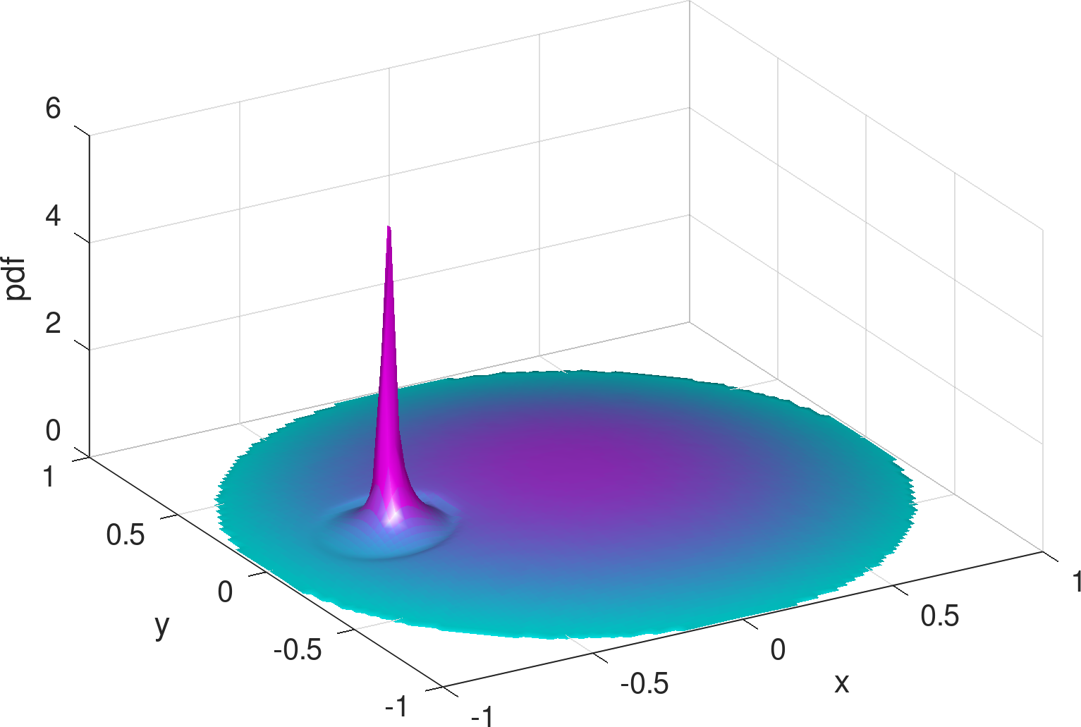
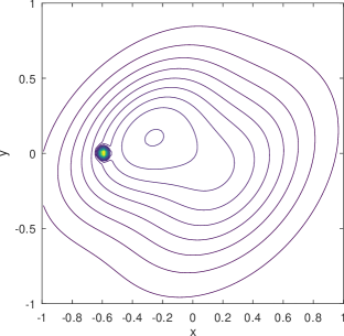
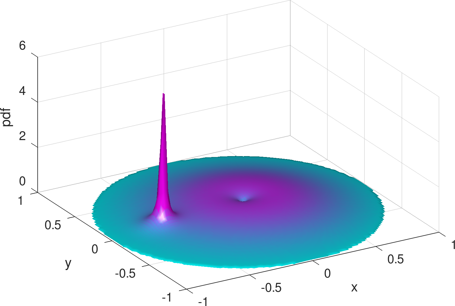
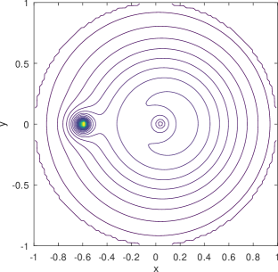
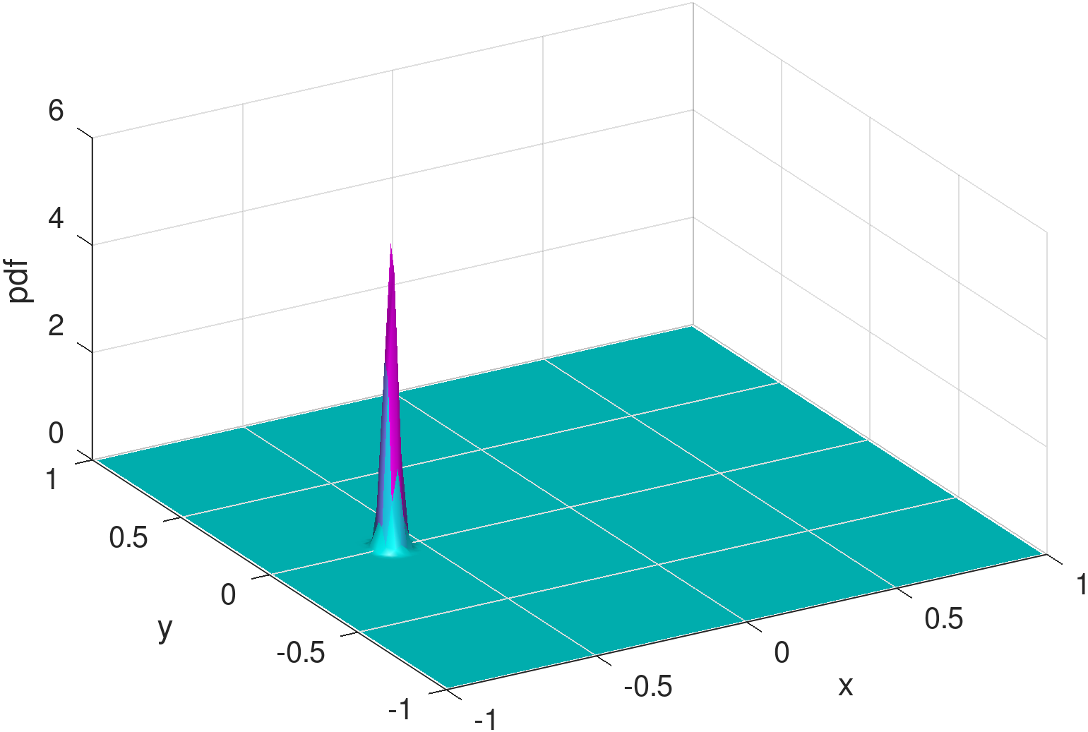
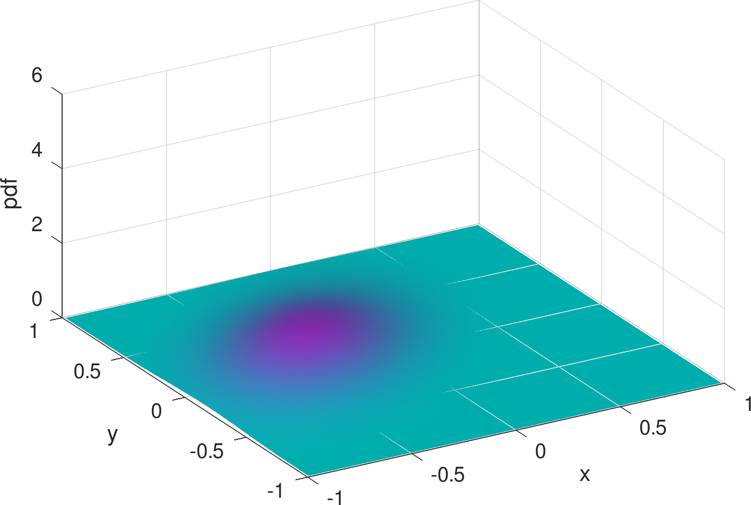
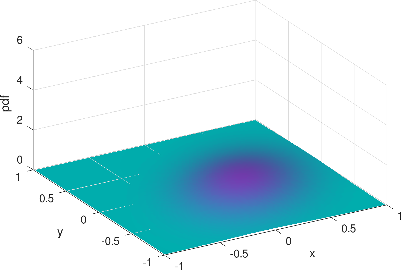
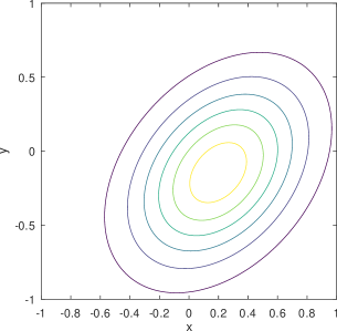
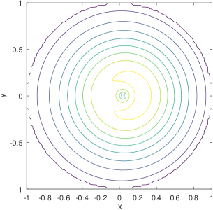
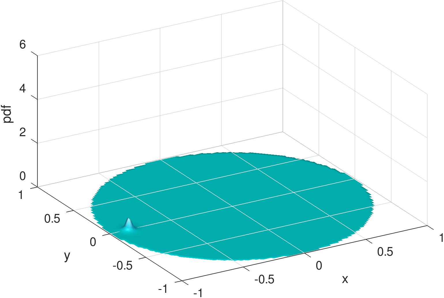
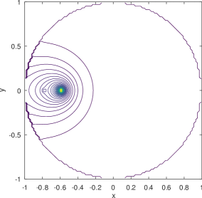
Existing mobility models range from simple random waypoint (RWP) to fairly elaborate models where nodes are attracted to specific regions/points because there exist spatial features. Closed-form analytical descriptions of the density rarely exist but only for a few cases, one such being the noted example of the RWP density [12]. An example of non-trivial density which lacks a closed-form solution and is computationally demanding even for its numerical approximation, is the one derived from the work in [8] and shown in the example of Figure 1. Zooming into the features of the distribution reveals subtleties like the density “peak” drops in a non-symmetric manner to the left and to the right of the peak, while at some distance around this peak there exists a “dip” in the density. The notable background “dome” is the RWP residual component of the distribution.
For an ML model to be convincing, it is necessary that it is also interpretable. The examples shown here illustrate what is a criterion for such interpretability. For example, a model that captures the RWP dome in one component distribution, and the off-center peak in another component can be claimed to be more interpretable than one that does not provide such separation.
The contributions of the current paper are all related to learning spatial distributions by means of mixtures of Möbius distributions and have the characteristics of:
-
•
capturing distributions defined on the disk, as required by many existing mobility models,
-
•
capturing distributions that include “features” such as local attraction points/peaks,
-
•
requiring a small number of training set data to produce a good model, and
-
•
resulting in component distributions that are more interpretable than Gaussians.
In Section 2 we provide a specific problem definition from the point of view of approximating a particular variety of density functions derived from mobility. The point is that a wider set of similar distributions can be handled using similar models. Section 3 introduces the family of Möbius distributions, in a mixture setting analogous to mixture-of-Gaussians, providing motivating examples of how (better) Möbius performs compared to Gaussians. The summary of learning results is given in Section 4 where we also comment on the fragility and worst-case outcomes of the Möbius mixtures compared to Gaussians. Section 5 links our work with a number of current trends in learning models comparing and contrasting them. Finally, Section 6 summarizes the paper and points to generalizations like non-circular boundaries, more general distributions, etc.
2 Motivation & Problem Definition
When engineering systems, such as communication systems, it is convenient to have closed-form formulations for relevant probability density functions and/or their related statistical properties. For example, the closed-form relation between the average delay and arrival rates at a queueing system, as per Little’s law, is often employed in solving bigger network design problems [13]. Here we are interested in aiding the solutions of spatial optimization problems, i.e., placement of resources, where the placement impacts a probability density function. Such optimization problems arise e.g., in the study of node density of mobile nodes moving around under certain mobility rules. Part of the assumptions when studying such spatial densities is how far is the extent of the space over which the distribution should be described. Motivated by the fact that many applications involve the placement of resources in cities and other population centers, an often applied assumption is that the area is circumscribed by a circle. Hence, densities over a disk are commonplace [14].
A well-studied baseline mobility model is the RWP model, which results in a closed-form probability density function of nodes across space [12]. RWP assumes that nodes continuously move around along straight paths from waypoint to next waypoint. Yet, when RWP is extended to capture more subtle movement rules, e.g., movement predicated on the state of the mobile nodes, and non-uniformity of space, extracting a closed-form solution is challenging. For example, RWP alone does not have a concept of points of attraction. Attraction points could be inflicting a change in the mobility behavior depending on the state and proximity of the mobile nodes. An example of this is the case of placing charging stations at specific locations and, as a result, attracting users to go to them to charge their mobile devices. One expects the density of mobile nodes to be higher around chargers. The less the overall available energy, the more the likelihood they will be attracted to the charger and the density will “bulge” around the charger which will influence their trip between successive waypoints. Deriving a function to describe the density based on pertinent parameters, e.g., location of the charger, average energy capacity of nodes, etc., is necessary in such an application.
In previous work [8], we have derived the node density distribution for a network of energy-constrained mobile nodes. We are repeating here some of the key formulas behind the analytical expression of the node density to illustrate their intertwined nature. Note that we have thus far found no closed-form solution for the distribution. Additionally, it is computationally expensive to produce a numerical approximation to the solution, in particular due to the multiple integrals involved. The purpose of the learning described in the next section is to learn an efficient function that evaluates to this complicated density using a small training set since each training point requires substantial numerical processing or lengthy simulations.
The density is a complicated one, owing to the fact that it models chargers that “attract” nodes whose energy is depleted. The trajectory of the mobile nodes is altered, from continuing to their destinations, to diverting to a charger before proceeding to their destinations. The decision to divert is only taken if the mobile node is a certain, relatively small, distance from the charger—equivalently seen as the “attraction” range of a charger. More formally, suppose that (our first two parameters) denotes the charger’s location in polar coordinates. That is, and are radial and angular coordinates respectively, where the radius of the disk (centered at (0,0)) is normalized to a unit (hence ). The (energy-depleted) mobile node will divert for recharging, provided that its current location, denoted by , is within the (closed) disk, , i.e., if it is within distance from the charger ( being the third parameter of our model). The limitation of attracting a depleted node only if it is within an attraction range models the reluctance of a node to divert significantly from their path to the destination for the sake of recharging (which they can do at their destination point anyway).
Besides adequate proximity to the charger, the other premise of the diversion for recharging, i.e., that the node is depleted, is made tantamount to the event that the node has traveled a distance ( is our fourth parameter) after departure from its last waypoint. This projection of energy consumption processes onto distance is a modeling convenience allowing us to lump together the effect of many factors (e.g., rated power, moving speed) into a typical “energy budget” expressed as a distance threshold , in the same units as those for determining the attraction () to the charger. An implicit assumption is that the energy for locomotion is separate from the energy for computation and communication—a scenario which fits the case of human movement with portable devices (e.g., smartphones, wearables) being carried around.
Even in the presence of a single charger, the formula we derived for the probability density is non–trivial and has so far evaded a closed form expression [8], leading to needs for numerical evaluation. Note that we have been able to derive closed form expressions for the 1-dimensional case [15], but its components and constraints are significantly less challenging than the 2-dimensional case. The following formula of node density for the 2-dimensional case applies when , i.e., when the charger is placed relatively close to the center to allow nodes that start moving from the boundary to have a chance to be attracted to the charger when their energy is depleted. The high-level structure of the spatial density satisfies the following equation:
| (1) |
where denotes the expected distance (including diversions to the charger) between any two waypoints, is the (stationary) probability density of the node’s location over time , and is the density assuming only RWP mobility (i.e., with no diversion to the charger).
Note that the movement area and thus the support of is a unit disk . The density within the attraction range of the charger (i.e., for ) can be captured, excluding the basic RWP component (and the coefficient ), by an infinity at the charger (i.e., for ) and a subtraction of two non-trivial functions and ; a similar superimposition onto , with the subtraction , is also found for formulating the nodal density beyond the attraction range (for ). The respective forms of , , , and are given by
| (2) | ||||
| (3) | ||||
| (4) | ||||
| (5) |
where
| (6) | ||||
| (7) | ||||
| (8) | ||||
| (9) |
and where , , , (), (), , , and are all lengths of line intervals between the node’s location (or, its current destination) and a certain intersection point along the node’s moving direction, with or without recharging at the charger. For instance, is the distance from the node’s location straight to the boundary of the (disk-shaped) movement area along its moving direction (at angle ), in the case of no need (or no opportunity) for recharging, while is the distance from to its original destination assuming that the node just departed from the charger, after recharging, for . Detailed illustration of the relevant line segments and other variables can be found in [8]. Nevertheless, the density function given by Equation 1 is too complicated to derive a closed-form expression for it. In fact, it might be computationally more convenient to perform simulations than attempt a numerical solution altogether! Yet, both simulation and numerical evaluation are undesirable when the density function is just a subroutine repetitively called from a larger optimization engine to solve a spatial placement problem.
The question we are trying to answer is, what learning technique could we employ to derive, from a small training set, an accurate node density distribution across the domain of interest (a disk in our case)? The parameters of this function will be the , , and as presented above. If indeed such a form is learned as a mixture of component distributions, we could also, depending on the learning technique used, tease out its constituent components, to gain further insights to the density distribution [8], especially if the components come from elementary well-understood functions, e.g., from Gaussians. To this end, we next focus on putting the research question in the context of learning mixtures of distributions.
3 Learning Mixtures: Gaussian vs. Möbius
The general framework of density learning based on mixtures of Gaussian (or Möbius for that matter) distributions can be found in Figure 2, which is inspired by the mixture density network (MDN) first introduced in [9]. The basic idea of MDNs is to approximate an unknown probability distribution conditioned on the input, through a weighted sum of distributions that are more manageable.
Note that Gaussian distributions are the most commonly assumed kernels in MDNs, since it has been proved that any density function in question can be approximated as accurately as possible by a Gaussian mixture model that is properly parameterized [16]. Despite the high flexibility and generality of Gaussian distributions, however, it remains an open question as to whether and how new distributions can be used to be better tailored (e.g., at a lower cost) to the needs of case-specific density approximations. In this paper, we answer the question of matching the finitely-supported density observed in (charging aware) mobile nodes by focusing and further elaborating on the (beta type III) Möbius distribution, which is introduced to substitute for the Gaussians.
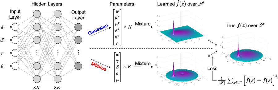
As seen in Figure 2, the input to the learning models is the 4-tuple characterizing an instance, i.e., , corresponding to the energy availability () of the node and the radius () and location (, ) of the charger (we start with the single-charger case). Through a fully connected deep neural network (containing two hidden layers of size in the example), a number of parameters, for Gaussian distributions (see Section 3.1), or parameters, for Möbius distributions (see Section 3.2), are produced at the output layer.
Regardless of whether we train for Gaussian or Möbius mixtures, the training loss function (Equation (10)) is evaluated over a set of density values sampled from the continuous derived distribution, at coordinate points defined by the set . While we are free to define set arbitrarily, our work is sampling uniformly on the x- and y- axis, along a grid.111That is, , following the same setting as in [8]. Only points within the circular support are of relevance to the density while points outside of it have zero density. For the loss function, we define
| (10) |
where denotes the density mixture obtained based on the learned parameters while is the ground truth acquired either by simulation or by numerical evaluation of the density in Equation 1. It is worth noting that we are not using the mean squared error (MSE) nor the Kullback–Leibler (KL) divergence for the loss measure, despite their prevalence in the literature. Instead, we consider the mean “quartic” error, i.e., the error of is raised to the power of 4, so as to enhance the ability to capture the “outlier”, which in this case is the peak of density around the charger’s location, as shown in Figures 1 and 2. MSE and KL divergence are used only as metrics of relative performance comparison in the experiments (see Section 4).
3.1 Mixture of Gaussians and Its Limitations
As illustrated in Figure 2, when (bivariate) Gaussian distributions are used as the kernels, the output layer of the neural network is of size , including mixing weights (), means (, ), standard deviations (, ), and correlation coefficients (). Although Gaussians are popular for mixture for mobility modeling [17, 18], the application of such classic distributions to our case has deficiencies that are critical to the efficacy of density approximation, as elaborated below.
1) Infinite support vs. encircled movement area. It is not hard to see that (basic) Gaussian distributions are infinitely supported, and hence their mixtures are bound to cause non-zero probability to “leak” out of the bounded movement area. One may consider truncating the distributions for a finite support [19], yet it is often non-trivial to evaluate the normalizing factors for truncation. To our understanding, there is no closed form for finding the exact truncated volume of an arbitrarily generated bivariate Gaussian over the unit disk (which is the finite support we assume). Alternatively, one may resort to numerical integration for approximate normalization. Nonetheless, as shown in Figure 1, the density distribution of the mobile node is characterized by zero-diminishing values approaching any point on the border of the disk, and it would take effort to keep this feature while imposing truncation on the Gaussians, be it exact or numerical for normalization.
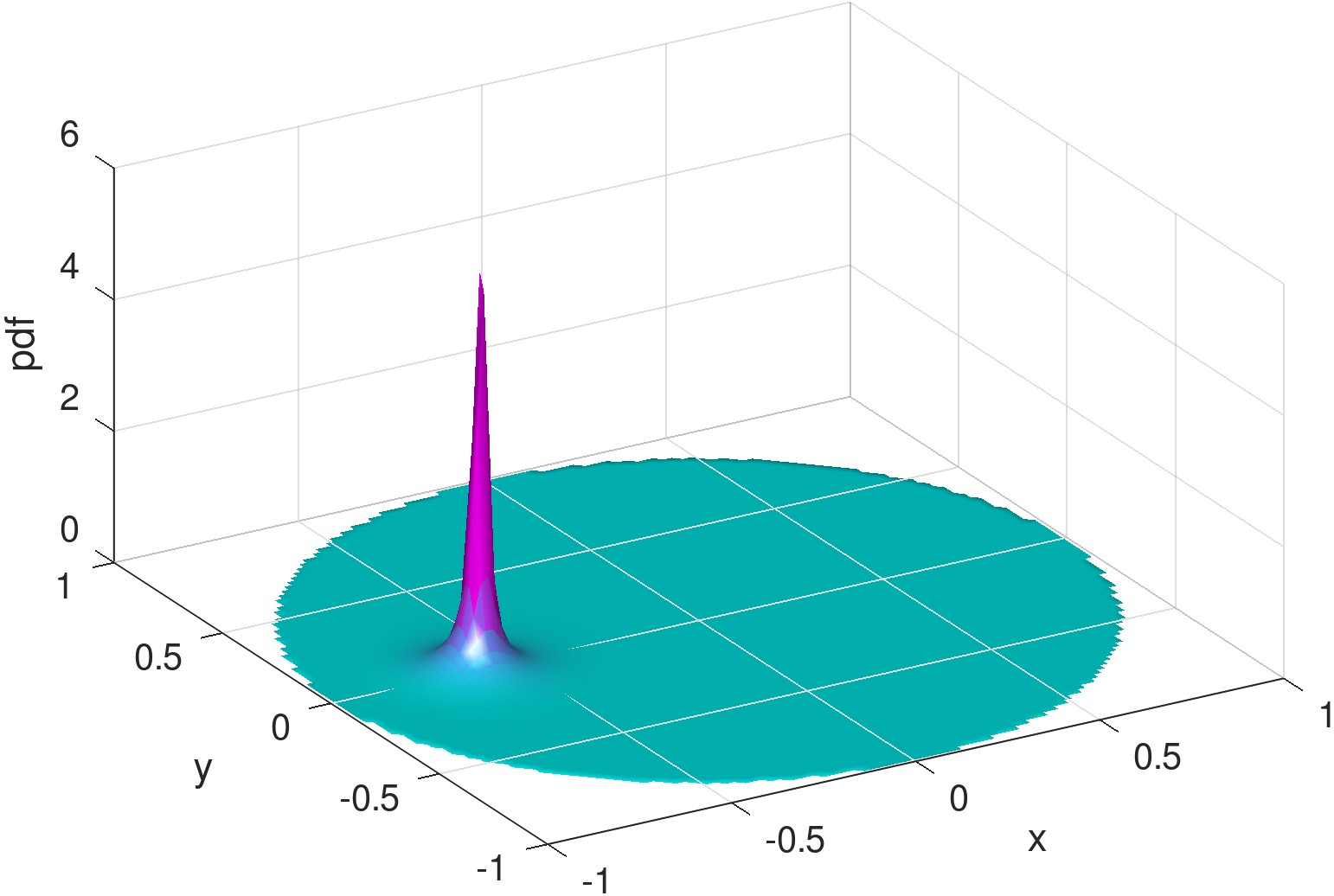
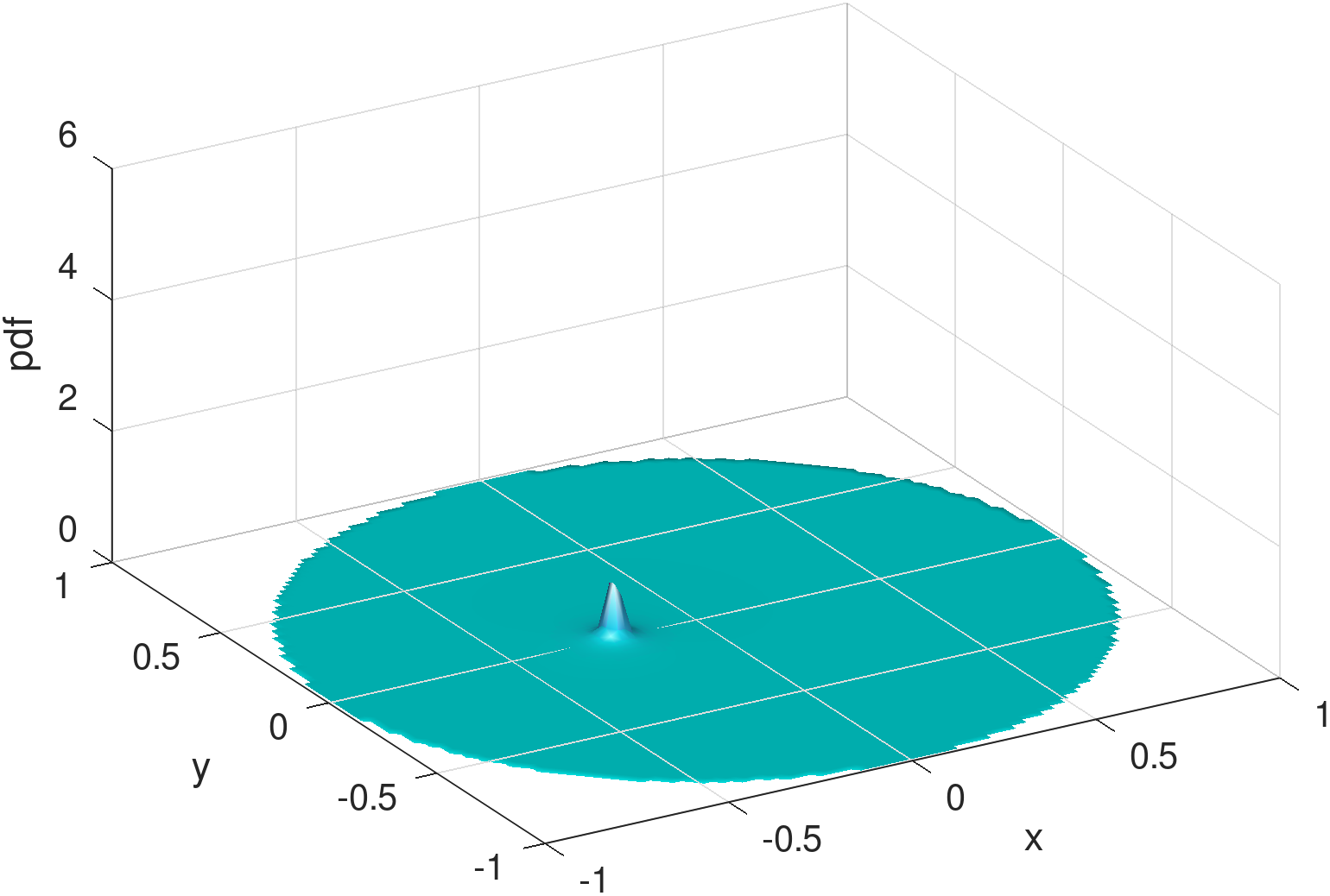
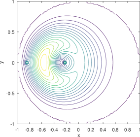
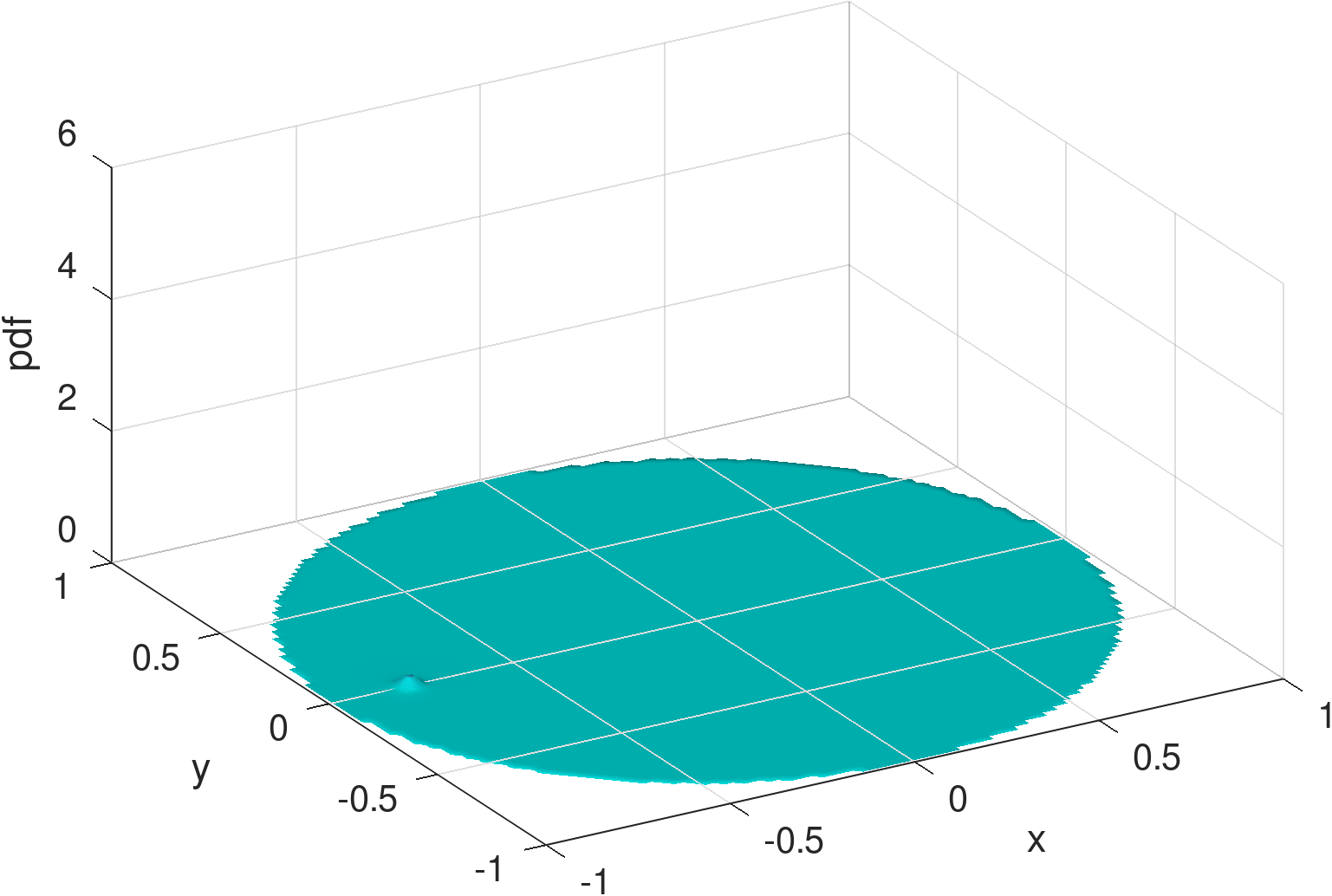
2) Bell surface vs. concave . The shapes of bivariate Gaussian distributions are subject to a particular bell surface, which is unnatural and inconvenient for fitting distributions that are radically different in shape. For illustration, Figure 3 exemplifies the output of the learning model from Figure 2 (see Section 4 for details and more results), assuming three Gaussians are mixed (i.e., ). In comparison to the exact density distribution in Figure 1, the fully trained Gaussian mixture model, despite capturing the surge at the charger location, appears to be poor at mimicking the RWP component, , which is spherically concave.
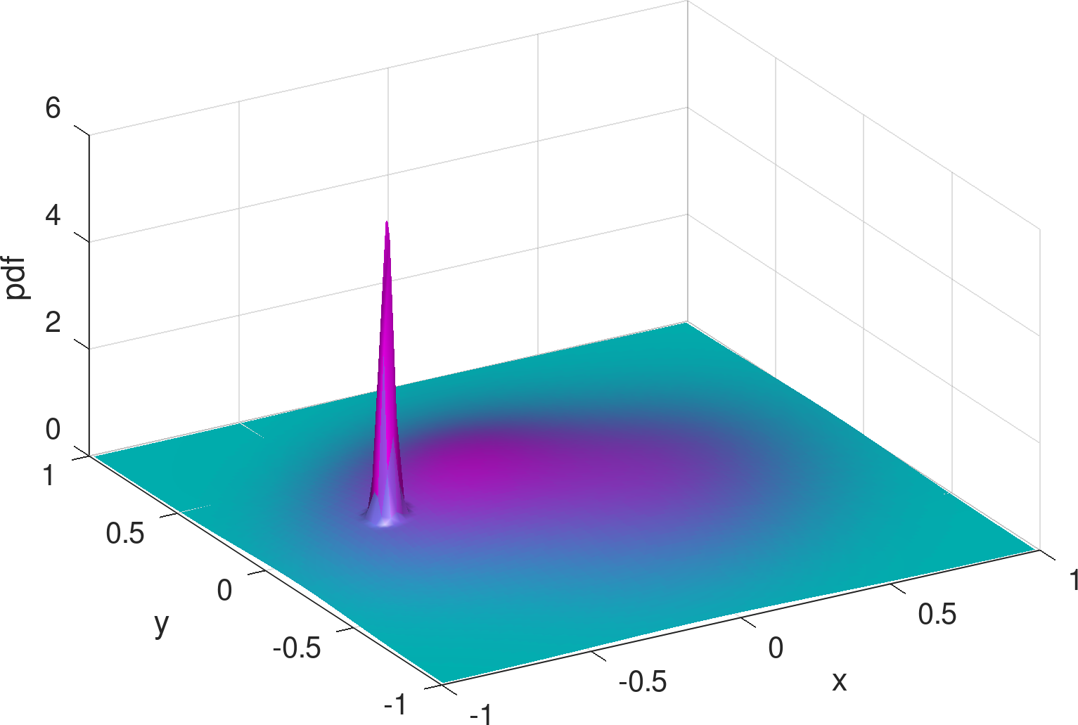
To delve into the reason, we can inspect the three Gaussian components separately, as shown in Figures 7 (a)–(f). Other than the spiky distribution around the charger, it can be seen that minimization of the loss function of Equation (10) gives rise to a scattering of two Gaussians over the movement area, for fitting . This is not surprising, since each Gaussian distribution is bell-shaped and thus needs multiple other Gaussians to be placed apart, on its outskirts, to complement the convexity around its tail areas. When the number of components is limited to three, with only two to fit , the convexity around either Gaussian component cannot be fully covered, resulting in the inadequate, long stretched dome in Figure 3.
3) More parameters vs. low-cost learning. A direct remedy for the limitation of bell-shaped Gaussians for approximating is to simply increase the number of components to be mixed. However, as we will see in Section 4 (e.g., Table 1), the gap in shape (in terms of the KL divergence) between the learned Gaussian mixture and the exact density distribution remains relatively wide even for increased up to 10 (i.e., 60 parameters to learn in total), while it entails scaling up the neural network proportionally to accommodate more parameters for output (noting that each hidden layer is of size ).
Another potential solution is to modify the Gaussian distribution somehow for better fitness. If one considers generalizing Gaussians for greater malleability, however, it can be costly (in terms of the number of parameters) since more additional parameters need to be introduced into each Gaussian component [20], adding to the parameters to estimate in total. On the other hand, it is non-trivial (if doable) to devise a specialized but simpler variant of the Gaussian distribution for our density fitting problem, while the susceptibility to an unbounded support still needs to be addressed. Hence, rather than tackle the conundrum faced by Gaussian distributions, it may be easier to find another suitable type of distribution that costs less for mixture.
3.2 Mixture of Möbius Distributions
To overcome the aforementioned deficiencies of the Gaussian mixture model and achieve good approximations with possibly fewer parameters, we make use of, as the kernel for mixture, the so-called beta type III Möbius distribution [21], which is an extended variant of the (basic) Möbius distribution originally proposed in [22]. The first key merit of this distribution is that it has a support of (in Cartesian coordinates), i.e., a unit disk, which exactly fits the support of the node density introduced in Section 2. Specifically, the beta type III Möbius distribution can be formulated as follows:
| (11) |
where
| (12) |
is the normalizing constant (with being the gamma function), and the four parameters, , , , and , control the steepness of concentration, modality (i.e., bimodality when and unimodality otherwise), skewness/asymmetry, and orientation of the distribution, respectively.
It is clear that the tuning of a beta type III Möbius distribution only involves four parameters, one parameter less than a Gaussian distribution. This is the second key merit of the Möbius distribution, i.e., having a relatively low cost of learning (in terms of the number of parameters), for a given value of . The third key merit of the Möbius-based mixture model, which may be less obvious, is its ability to emulate the shape of the node density that we are concerned with, despite fewer parameters used.
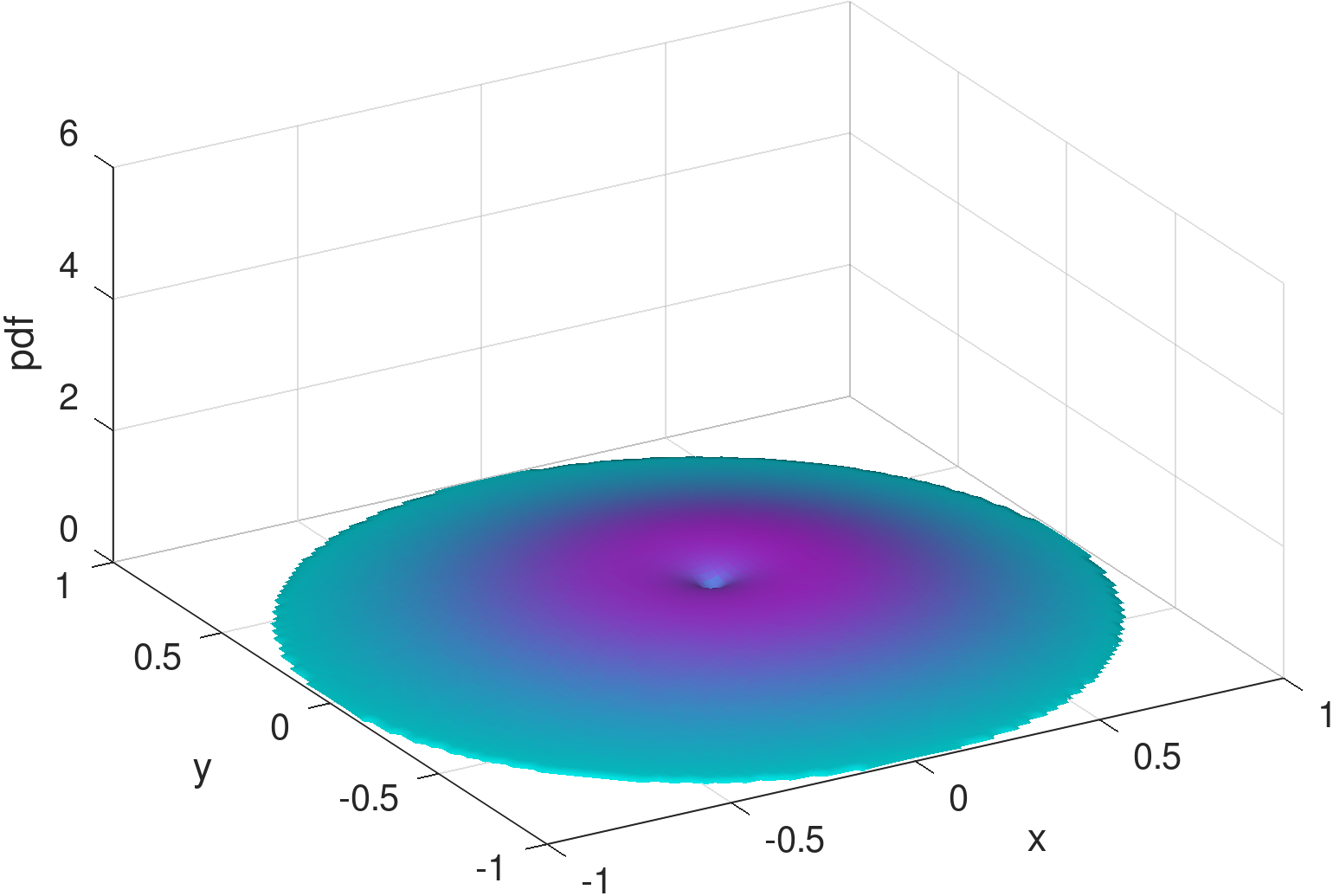
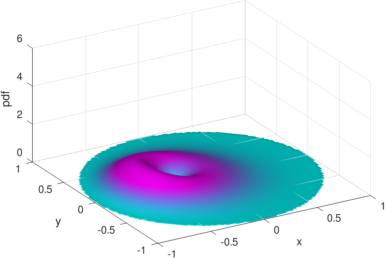
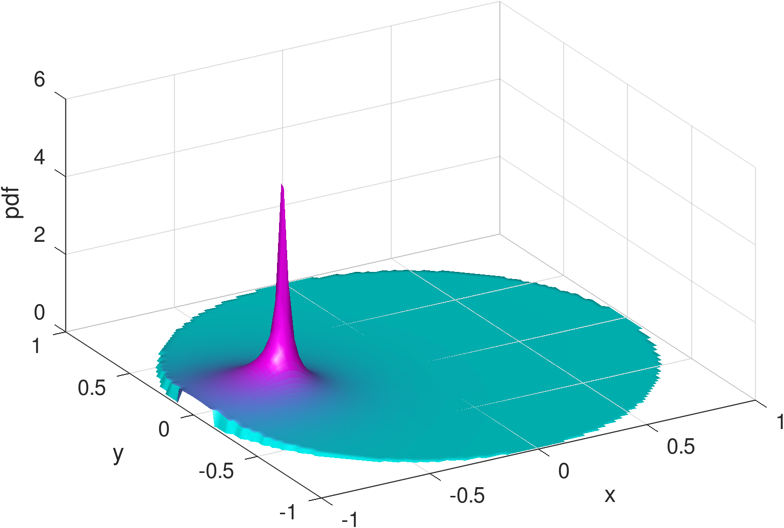
As a hint, Figure 4 shows the distribution mixed from three beta type III Möbius distributions that are sufficiently tuned by the learning model. Besides capturing the spike at the charger, it can be seen that the shape of the learned density using Möbiuses can well retain the concavity (although with a minor dimple around the origin) and symmetry of the RWP component, , visually appearing superior to the Gaussian mixture model (Figure 3). The superiority is confirmed by the numerical results, i.e., the KL divergence of the exact density distribution (Figure 1) from the mixed Möbiuses can decrease to 0.0219, far lower than the value of 0.1048 from the mixed Gaussians. The Möbiuses are also better in terms of MSE, with .
| 1 | 2 | 3 | 4 | 5 | 6 | 7 | 8 | 9 | 10 | ||
| Gaussian | Params. | 5 (5) | 10 (12) | 15 (18) | 20 (24) | 25 (30) | 30 (36) | 35 (42) | 40 (48) | 45 (54) | 50 (60) |
| MSE | |||||||||||
| KL | |||||||||||
| Möbius | Params. | 4 (4) | 08 (10) | 12 (15) | 16 (20) | 20 (25) | 24 (30) | 28 (35) | 32 (40) | 36 (45) | 40 (50) |
| MSE | |||||||||||
| KL |
4 Evaluation Results
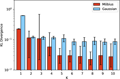
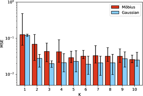
The results shown here are the outcome of ten separate training sessions using a training set of only five examples. A summary of the training results across training sessions is shown in Table 1 where the columns indicate the use of a different number, , of distributions mixed. The row Params. lists the number of determining parameters needed by each model, which is for Gaussian (mean and variance for x- and y-axis, as well as covariance) and for Möbius (, , , and ), and the numbers in parentheses is the number inclusive of the additional weight parameters when . The results are shown both in terms of MSE and KL-divergence, evaluated over the set , accompanied by 95% confidence intervals. Given that the training data set is the same, the benefit of using Möbius is obvious under a KL-divergence metric; a distinction in terms of MSE is less obvious. The improved KL score suggests a better matching of the “shape” of the distribution using Möbius.

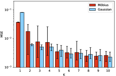
The same results are plotted in Figure 5 albeit the errorbars indicate the range from minimum to maximum performance across the ten independent training runs. In terms of variability of training, the KL-divergence again points to a better albeit more variable outcome for Möbius at small . Yet, for the KL-divergence range of results is almost always non-intersecting with the range of results from the corresponding Gaussian. Again, the MSE results do not allow for a more crisp separation between Gaussian and Möbius.
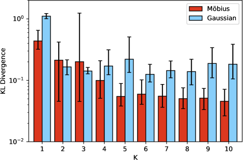
A demonstration that the training has been effective can be witnessed in the prediction results shown in Figure 6 which presents the average MSE and KL-divergence for the distribution prediction for 25 different parameter settings not present in the training set. The results appear similar, and occasionally better compared to the training results in terms of KL-divergence for Möbius (for ) over Gaussian mixtures. The good observed generalization performance suggests that the models do not overfit to the, small as it is, training data set.
The inability of the Gaussian mixture to mimic the density distribution can be explained by considering the shape of the constituent distributions. As an example, the Gaussian distributions () plotted in the two first rows of Figure 7 are superposed to produce the result shown in Figure 3 for a point belonging to the training set. While the peak at the charger’s location is captured, that is the limit of how interpretable the Gaussian results can be. The remaining background “dome” of the distribution is poorly reconstructed by the two remaining Gaussians both of which are haphazard in their placement. While the MSE of this mixture may indeed be small, its shape (and its KL-divergence) leaves a lot to be desired, lacking the symmetries we would expect to see in a better quality reconstruction.
The Möbius distributions (), on the other hand, for the exact same training set input, corresponding to the bottom two rows of Figure 7 combined to produce Figure 4, are quite capable of capturing the requisite symmetries and be very interpretable. One Möbius distribution corresponds to the charger peak feature, and another one corresponds to the main RWP dome feature, with additional distributions contributing to enhance either one of the two features. Albeit it is also evident that at is the cusp of sufficiently good Möbius-based reconstruction as the error bars in Figure 5 attest. To this end we provide examples of the worst Möbius reconstructions for collected during our runs for points in the training set.
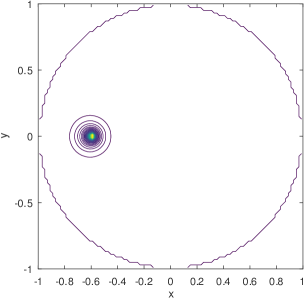
Figure 8 is for exhibiting an MSE of 0.0177 and KL-divergence of 0.1228. Figure 9, for the same parameters shows an MSE of 0.0276 and KL-divergence of 0.6863. Figure 8 captures an instance of a failure to capture the peak at the charger while able to capture a significant part of the mass on the main dome (Figure 8). Figure 9 represents the opposite behavior, where the density around the charger is captured (Figure 9) but not the main dome. As we comment next, the training phase for Möbius can be fragile owing to the interplay of the parameters and sub-expressions that define it.

4.1 Model Training Performance
The mixture model (either Gaussian or Möbius) accepts as input a batch of five 4-vectors, i.e., , , , , and , following . Each epoch includes (only) one batch, and the training would terminate when the change of the loss value remains less than for 400 epochs. The average numbers of epochs (over all runs) before convergence are shown to be around 3029 and 1844 for the Gaussian and Möbius mixture models, respectively. Regarding the coordinates for sampling, the set (Equation (10)) includes the points outside of the disk. By forcing the ground-truth distribution to have zero mass there, pressure is exerted on the Gaussian mixture to place the distribution so that they do not leak as much outside of the disk. Moreover, given the finite support of the Möbius distribution, the Möbiuses are forced to evaluate to zero outside of the disk.
For the optimizer, we use Adam (Adaptive Moment Estimation) instead of SGD (Stochastic Gradient Descent), with the learning rate set to 0.005. The preference for Adam is based on the observation from our experiments that both the Gaussian and Möbius mixture models, if optimized by SGD, would be susceptible to notable underfitting during training, even with carefully tuned momentums. Such occurrences of underperformance with SGD are also reported in [23]. Note that the Adam optimizer may cause learning models (especially those of great depths) to produce divergent training loss values, as recently investigated in [24]. This instability of Adam can potentially add to the variability shown in the results of the Möbius mixture model (e.g., see Table 1, when ).
Speaking of why training Möbiuses is more unstable than training Gaussians in our experiments, we find that the density values induced by Möbius mixtures can be destabilized easily by “unfortunate” settings of coordinates and parameters that tend to blow up certain terms of Equation 11. For instance, the term, , may be evaluated as infinity for coordinates , provided that both and are sufficiently close to zero. This sensitivity also applies to other terms of Equation 11, e.g., and .
A remedy for this issue is to intentionally exclude certain instability-prone ranges of the coordinate-parameter combinations. While this may be relatively easy when dealing with , it is more intricate and challenging for the other two terms mentioned. More sophisticated remedies are to be considered in future work [25].
4.2 Prediction Computation Performance
The benefits of a trained model can be better appreciated in the context of the running time required to determine the distribution for a given set of . We use an Intel i7-8700 system with Windows 11 and Windows Subsystem for Linux (WSL) 2 hosting Ubuntu 22.04.5. No GPU is used, and no explicit parallelism is programmed or requested, hence the running times quoted here are for single-core sequential execution:
-
•
a single numerical evaluation of Equation 1 in MATLAB R2024b running natively on Windows 11 without any MATLAB parallelism directives, takes approximately 108 minutes,
-
•
a single simulation of the system behavior using a custom-made C++ simulator for a total traveled normalized222The disk radius is the normalized unit of distance. distance of units (gcc 11.4.0, -O3 optimization, on WSL2) takes approximately 13 minutes,
-
•
a single inference/prediction invocation using Python (python 3.11.5, numpy 2.1.1, torch 2.4.1+cu121, on WSL2) without any GPU support, takes approximately 7 milliseconds.
Clearly the produced model is several orders of magnitude faster than the other two options. Note that the MATLAB code is executed with defaults for the numerical evaluation accuracy, e.g.. those impacting integration. The Python inference times do not include the model loading time, which is assumed already present in memory. In any application the cost of loading the model is amortized across the multiple invocations to the inference function.
From a single simulation run we extract ten successive measurements of the density distribution, with each measurement corresponding to a traveled distance of units, adding up to the total of units. This is done to introduce a number of measurements of density out of a single run, with each measurement incorporating a degree of “noise” around the steady-state values. Having multiple, similar, but noisy inputs is a well-known approach to combat over-fitting in learned models. While the simulation time can be reduced proportionally to reduce the simulated distance traveled, it was observed that the measured density deteriorates significantly if the density measurement intervals were reduced below units.
5 Related Work
The problem under consideration falls under the general category of inverse problems, i.e., problems where the observed data are assumed to come from a function whose parameters need to be derived. Solving inverse problems using learning algorithms has met with some success in various domains in the natural sciences [26, 27, 28]. The shape of the density function seen in [8] and [15] suggest a rather well-behaving, continuous and smooth function with the notable exception of the singular point at the exact location of the charger(s). Nevertheless, it is difficult to find a tractable density function that fits the shape while being analytic, and we resort to mixture models, although the choice of a suitable kernel distribution is still non-trivial. Note that our attention is given to inverse modeling, meaning the derivation of a closed form is considered as valuable, not only for accelerating the simulation process but also for facilitating further mathematical analyses of network performance (e.g., wireless capacity [15]). Hence, we disregard the class of sampling-based generative models (e.g., [29]) that can only numerically output the density value given the location.
To our understanding, such spatial density learning using finite-supported, non-Gaussian mixtures for improving mobility modeling and simulation is still lacking in the networking community. There are related studies on Gaussian-based mixture density learning for urban transportation, whose interests or assumptions are nevertheless at variance with our work. For instance, in order to alleviate traffic congestion in urban areas, the GPS traces of over 1,000 taxis in a city are analyzed in [18], where a Gaussian mixture model is adopted to model the taxis’ location distribution for hotspot evaluation. The mobility considered there is constrained, in the sense that the traces are limited to graph-like road networks. This is different from our assumption of a bounded circular movement area in the Euclidean plane. In [30], the patterns of cellphone users, who have transitional states of location driven by temporal periodicity and social interplay, are modeled by mixing pairs of Gaussians (accounting for periodicity), together with a power-law distribution (for social dynamics). In their example, the spatial model assumes a square-shaped support for mobility, but it is unclear how the potential density leakage is addressed. Also, the number of component distributions is supposedly fixed in [30]. In [31], Gaussian kernels with adaptive bandwidths (parameterizing the correlation matrices) are introduced for estimating spatial density of mobile users at different scales. The bandwidths are adapted by the kernel density estimation method to account for density discrepancy between highly (e.g., roads) and sparsely (e.g., deserts) populated areas. Like [18, 30], the focus is mainly on accommodating the heterogeneous dependence of density on locations, with no concern or solution for fitting specifically confined movement areas.
The application of non-Gaussian mixtures, with finite or semi-finite supports, appears to be more common in learning non-geographic density distributions. Such applications have occurred in various domains like astrophysics [32], economics [33], and power engineering [34]. For instance, beta distributions (with a support of ) are mixed in [32] to infer cosmological parameters of one-dimensional CDM (cold dark matter) models. The betas are also employed in [34] for an improved MDN such that the univariate wind power output of wind farms can be forecast with no issue of density leakage. In [33], an MDN using the multivariate Gamma distribution (having a support of for each marginal variable) as its kernel is proposed to model the distribution of insurance claim amounts. The methods mentioned above are certainly not applicable to our scenario of mobility modeling for mobile networks.
The Möbius-based mixture learning model we have proposed is inspired by the work of [21], where a new class of disk-supported distributions (including the beta type III Möbius distribution) is proposed to model the bivariate density of wind speed and wind direction over Marion Island. Their work focuses on deriving fitted distribution forms for accurate wind modeling, making no mention of density mixture for potential fitness improvement.
Lastly, it is worth mentioning another type of mixture density learning problem that is often considered in autonomous driving and robot navigation, e.g., [35, 36, 37], which appear to be related but are in essence distinct from our scenario. There, the basic idea is to use mostly Gaussian and occasionally non-Gaussian (e.g., Laplacian [36]) mixture models to predict near-future trajectories of vehicles or robots in the locality (e.g., at an intersection) given a relatively short past history (e.g., within seconds), such that the moving agents can navigate efficiently and safely without collision. As can be seen, the main concern of such studies is prescriptive route planning or maneuver control at relatively small scales in both spatial and temporal aspects, or equivalently, involving one or at most a few pairs of random “waypoints” in the whole learning process. In contrast, the (disk-shaped) movement area we have assumed can be as broad as a city, and the span of a nodal trajectory simulated corresponds to the node moving for extended periods of time such that a steady state can be reached. Therefore, applying short-term prediction methods is at odds with our steady-state based problem formulation.
6 Conclusions
We have demonstrated the usefulness of Möbius distributions as component distributions for mixed density networks, as it pertains to capturing distributions of mobile nodes confined on disks. The results are promising in the sense that they produce small, interpretable models that retain the symmetries present in such distributions. Our objective is to use the learned model as a subroutine in an optimization task, e.g., a charger location assignment problem. The methodology we followed exposes also several shortcomings and areas for future improvement.
As mentioned in Section 4.1, the stability of general purpose optimizers like Adam for MDNs of Möbius distributions is relatively poor. We will pursue alternatives, e.g., based on particular forms of regularization [25]. Another extension will be towards distributions with other (non-disk) forms of support, e.g., rectangular or square, as they are also often seen in mobile network performance studies.
It is also worth pointing out that extensions can be applied also when some of the density-influencing parameters are stochastic, rather than constants. As an example, the distance which acts as a proxy of energy availability upon departure from a waypoint, can be replaced by distributions with a mean , and there may be benefit to also include higher moments of such distributions.
References
- [1] A. Mestres, E. Alarcón, Y. Ji, and A. Cabellos-Aparicio, “Understanding the modeling of computer network delays using neural networks,” in Proceedings of the 2018 Workshop on Big Data Analytics and Machine Learning for Data Communication Networks, ser. Big-DAMA ’18, 2018, pp. 46–52.
- [2] M. Ferriol-Galmés, J. Paillisse, J. Suárez-Varela, K. Rusek, S. Xiao, X. Shi, X. Cheng, P. Barlet-Ros, and A. Cabellos-Aparicio, “Routenet-fermi: Network modeling with graph neural networks,” IEEE/ACM Trans. Netw., vol. 31, no. 6, pp. 3080–3095, May 2023.
- [3] S. Huang, Y. Wei, L. Peng, M. Wang, L. Hui, P. Liu, Z. Du, Z. Liu, and Y. Cui, “xnet: Modeling network performance with graph neural networks,” IEEE/ACM Transactions on Networking, vol. 32, no. 2, pp. 1753–1767, 2024.
- [4] S. Szott, K. Kosek-Szott, P. Gawłowicz, J. T. Gómez, B. Bellalta, A. Zubow, and F. Dressler, “Wi-fi meets ml: A survey on improving ieee 802.11 performance with machine learning,” IEEE Communications Surveys & Tutorials, vol. 24, no. 3, pp. 1843–1893, 2022.
- [5] K. Kawaguchi, L. P. Kaelbling, and Y. Bengio, “Generalization in deep learning,” In Mathematical Aspects of Deep Learning. Cambridge University Press, 2022.
- [6] J.-Y. Le Boudec, “Understanding the simulation of mobility models with palm calculus,” Performance evaluation, vol. 64, no. 2, pp. 126–147, 2007.
- [7] J. Treurniet, “A taxonomy and survey of microscopic mobility models from the mobile networking domain,” ACM Computing Surveys (CSUR), vol. 47, no. 1, pp. 1–32, 2014.
- [8] W. Gao, I. Nikolaidis, and J. J. Harms, “On the impact of recharging behavior on mobility,” IEEE Transactions on Mobile Computing, vol. 22, no. 7, pp. 4103–4118, 2023.
- [9] C. M. Bishop, “Mixture density networks,” Aston University, Tech. Rep. NCRG/94/004, 1994.
- [10] K. N. Plataniotis and D. Hatzinakos, “Gaussian mixtures and their applications to signal processing,” Advanced signal processing handbook, pp. 89–124, 2017.
- [11] I. Goodfellow, Y. Bengio, and A. Courville, Deep Learning. MIT Press, 2016.
- [12] E. Hyytia, P. Lassila, and J. Virtamo, “Spatial node distribution of the random waypoint mobility model with applications,” IEEE Transactions on mobile computing, vol. 5, no. 6, pp. 680–694, 2006.
- [13] D. Malak, A. Cohen, and M. Médard, “How to distribute computation in networks,” in IEEE Conference on Computer Communications, ser. INFOCOM ’20, 2020, pp. 327–336.
- [14] X.-Y. Yan, W.-X. Wang, Z.-Y. Gao, and Y.-C. Lai, “Universal model of individual and population mobility on diverse spatial scales,” Nature Communications, vol. 8, no. 1, p. 1639, 2017.
- [15] W. Gao, I. Nikolaidis, and J. J. Harms, “On the interaction of charging-aware mobility and wireless capacity,” IEEE Transactions on Mobile Computing, vol. 19, no. 3, pp. 654–663, 2020.
- [16] G. J. McLachlan and K. E. Basford, Mixture models: Inference and applications to clustering. M. Dekker New York, 1988, vol. 38.
- [17] L. Alessandretti, U. Aslak, and S. Lehmann, “The scales of human mobility,” Nature, vol. 587, no. 7834, pp. 402–407, 2020.
- [18] J.-j. Tang, J. Hu, Y.-w. Wang, H.-l. Huang, and Y.-h. Wang, “Estimating hotspots using a gaussian mixture model from large-scale taxi gps trace data,” Transportation Safety and Environment, vol. 1, no. 2, pp. 145–153, 2019.
- [19] M. Azam, “Bounded support finite mixtures for multidimensional data modeling and clustering,” Ph.D. dissertation, Concordia University, 2019.
- [20] L. Arnroth, “Some investigations into the class of exponential power distributions,” Ph.D. dissertation, Acta Universitatis Upsaliensis, 2023.
- [21] A. Bekker, P. Nagar, M. Arashi, and H. Rautenbach, “From symmetry to asymmetry on the disc manifold: Modeling of marion island data,” Symmetry, vol. 11, no. 8, 2019.
- [22] M. Jones, “The möbius distribution on the disc,” Annals of the Institute of Statistical Mathematics, vol. 56, no. 4, pp. 733–742, 2004.
- [23] A. C. Wilson, R. Roelofs, M. Stern, N. Srebro, and B. Recht, “The marginal value of adaptive gradient methods in machine learning,” in Proceedings of the 31st International Conference on Neural Information Processing Systems, ser. NIPS ’17, 2017, pp. 4151–4161.
- [24] I. Molybog, P. Albert, M. Chen, Z. DeVito, D. Esiobu, N. Goyal, P. S. Koura, S. Narang, A. Poulton, R. Silva et al., “A theory on adam instability in large-scale machine learning,” arXiv preprint arXiv:2304.09871, 2023.
- [25] L. U. Hjorth and I. T. Nabney, “Regularisation of mixture density networks,” in Ninth International Conference on Artificial Neural Networks, ser. ICANN ’99. IET, 1999, pp. 521–526.
- [26] K. Xu and E. Darve, “Solving inverse problems in stochastic models using deep neural networks and adversarial training,” Computer Methods in Applied Mechanics and Engineering, vol. 384, p. 113976, 2021.
- [27] S. Cuomo, V. S. Di Cola, F. Giampaolo, G. Rozza, M. Raissi, and F. Piccialli, “Scientific machine learning through physics–informed neural networks: Where we are and what’s next,” Journal of Scientific Computing, vol. 92, no. 3, p. 88, 2022.
- [28] J. Gilmer, S. S. Schoenholz, P. F. Riley, O. Vinyals, and G. E. Dahl, “Neural message passing for quantum chemistry,” in Proceedings of the 34th International Conference on Machine Learning, ser. ICML ’17, vol. 70, 2017, pp. 1263–1272.
- [29] D. Gammelli and F. Rodrigues, “Recurrent flow networks: A recurrent latent variable model for density estimation of urban mobility,” Pattern Recognition, vol. 129, p. 108752, 2022.
- [30] E. Cho, S. A. Myers, and J. Leskovec, “Friendship and mobility: user movement in location-based social networks,” in Proceedings of the 17th ACM SIGKDD International Conference on Knowledge Discovery and Data Mining, ser. KDD ’11, 2011, pp. 1082–1090.
- [31] M. Lichman and P. Smyth, “Modeling human location data with mixtures of kernel densities,” in Proceedings of the 20th ACM SIGKDD International Conference on Knowledge Discovery and Data Mining, ser. KDD ’14, 2014, pp. 35–44.
- [32] G.-J. Wang, C. Cheng, Y.-Z. Ma, and J.-Q. Xia, “Likelihood-free inference with the mixture density network,” The Astrophysical Journal Supplement Series, vol. 262, no. 1, p. 24, 2022.
- [33] Ł. Delong, M. Lindholm, and M. V. Wüthrich, “Gamma mixture density networks and their application to modelling insurance claim amounts,” Insurance: Mathematics and Economics, vol. 101, pp. 240–261, 2021.
- [34] H. Zhang, Y. Liu, J. Yan, S. Han, L. Li, and Q. Long, “Improved deep mixture density network for regional wind power probabilistic forecasting,” IEEE Transactions on Power Systems, vol. 35, no. 4, pp. 2549–2560, 2020.
- [35] O. Makansi, E. Ilg, O. Cicek, and T. Brox, “Overcoming limitations of mixture density networks: A sampling and fitting framework for multimodal future prediction,” in Proceedings of the IEEE/CVF Conference on Computer Vision and Pattern Recognition, ser. CVPR ’19, 2019, pp. 7144–7153.
- [36] Z. Zhou, J. Wang, Y.-H. Li, and Y.-K. Huang, “Query-centric trajectory prediction,” in Proceedings of the IEEE/CVF Conference on Computer Vision and Pattern Recognition, ser. CVPR ’23, 2023, pp. 17 863–17 873.
- [37] S. Choi, K. Lee, S. Lim, and S. Oh, “Uncertainty-aware learning from demonstration using mixture density networks with sampling-free variance modeling,” in 2018 IEEE International Conference on Robotics and Automation, ser. ICRA ’18, 2018, pp. 6915–6922.