Beyond Regret: Decoupling Learning and Decision-making in Online Linear Programming
Abstract
Online linear programming plays an important role in both revenue management and resource allocation, and recent research has focused on developing efficient first-order online learning algorithms. Despite the empirical success of first-order methods, they typically achieve a regret no better than , which is suboptimal compared to the bound guaranteed by the state-of-the-art linear programming (LP)-based online algorithms. This paper establishes a general framework that improves upon the result when the LP dual problem exhibits certain error bound conditions. For the first time, we show that first-order learning algorithms achieve regret in the continuous support setting and regret in the finite support setting beyond the non-degeneracy assumption. Our results significantly improve the state-of-the-art regret results and provide new insights for sequential decision-making.
1 Introduction
This paper presents a new algorithmic framework to solve the online linear programming (OLP) problem. In this context, a decision-maker receives a sequence of resource requests with bidding prices and sequentially makes irrevocable allocation decisions for these requests.
OLP aims to maximize the accumulated reward subject to inventory or resource constraints. OLP plays an important role in a wide range of applications. For example, in online advertising [4], an online platform has limited advertising slots on a web page. When a web page loads, online advertisers bid for ad placement, and the platform decides within milliseconds the slot allocation based on the features of advertisers and the user. The goal is to maximize the website’s revenue and improve user experience. Another example is online auction, where an online auction platform hosts a large number of auctions for different items. The platform must handle bids and update the auction status in real-time. Besides the aforementioned applications, OLP is also widely used in applications such as revenue management [29], resource allocation [15], cloud computing [12], and many other applications [3].
Most state-of-the-art algorithms for OLP are dual linear program (LP)-based
[1, 16, 22, 19, 22]. More specifically, these algorithms require solving a sequence of LPs to make online decisions. However, the high computational cost of these LP-based methods prevents their application in time-sensitive or large-scale problems. For example, in the aforementioned online advertising example, a decision has to be made in milliseconds, while LP-based methods can take minutes to hours on large-scale problems. This challenge motivates a recent line of research
using first-order methods to address OLP
[18, 10, 4, 5], which are based on gradient information and more scalable and computationally efficient than LP-based methods.
Despite the advantage in computational efficiency, first-order methods are still not comparable to LP-based methods in terms of regret for many settings. Existing first-order OLP algorithms only achieve regret bound with only a few exceptions. When the distribution of requests and bidding prices has finite support [28], regret is obtainable using a three-stage algorithm; if first-order methods are used to solve the subproblems of LP-based methods infrequently, regret is achievable in the continuous support setting under a uniform non-degeneracy assumption [22]. However, these methods are either complicated to implement or require strong assumptions. It remains open whether there exists a general framework that allows first-order methods to break the regret barrier. This paper answers this question affirmatively.
1.1 Contributions
-
•
We show that first-order methods achieve regret under weaker assumptions than LP-based methods. In particular, we identify a dual error bound condition that is sufficient to guarantee lower regret of first-order methods when the dual LP problem has a unique optimal solution. In the continuous-support setting, we establish an regret result under weaker assumptions than the existing methods; In the finite-support setting, we establish an result, which significantly improves on the state-of-the-art result and almost matches the regret of LP-based methods. For problems with -Hölder growth condition, we establish a general regret result, which interpolates among the settings of no growth (), continuous support with quadratic growth () and finite support with sharpness (). Our results show that first-order methods perform well under strictly weaker conditions than LP-based methods and still achieve competitive performance, significantly advancing their applicability in practice.
-
•
We design a general exploration-exploitation framework to exploit the dual error bound condition. The idea is to learn a good approximation of the distribution dual optimal solution. Then, the online decision-making algorithm can be localized around a neighborhood of the approximate dual solution and makes decisions in an effective domain of size , thereby achieving improved regret guarantees. We reveal an important dilemma in simultaneously using a single first-order method as both learning and decision-making algorithms: a good learning algorithm can perform poorly in decision-making. This dilemma implies an important discrepancy between stochastic optimization and online decision-making, and it is addressed by decoupling learning and decision-making: two different first-order methods are adopted for learning and decision-making. This simple idea yields a highly flexible framework for online sequential decision-making. Our analysis can be of independent interest in the broader context of online convex optimization.
| Paper | Setting and assumptions | Algorithm | Regret | Lower bound |
| [19] | Bounded, continuous support, uniform non-degeneracy | LP-based | Yes | |
| [7] | Bounded, continuous support, uniform non-degeneracy | LP-based | Yes | |
| [13] | Bounded, finite support of , quadratic growth | LP-based | Unknown | |
| [22] | Bounded, continuous support, uniform non-degeneracy | LP-based | Yes | |
| [9] | Bounded, finite support, non-degeneracy | LP-based | Yes | |
| [18] | Bounded | Subgradient | Yes | |
| [4] | Bounded | Mirror Descent | Yes | |
| [10] | Bounded | Proximal Point | Yes | |
| [5] | Bounded | Momentum | Yes | |
| [28] | Bounded, finite support, non-degeneracy | Subgradient | No () | |
| [22] | Bounded, continuous support, uniform non-degeneracy | Subgradient | No () | |
| This paper | Bounded, continuous support, quadratic growth | Subgradient | No () | |
| This paper | Bounded, finite support, sharpness | Subgradient | No () | |
| This paper | Bounded, -dual error bound, unique solution | Subgradient | Unknown |
Related Literature.
There is a vast amount of literature on OLP [23, 25, 24, 2], and we review some recent developments that go beyond regret in the stochastic input setting (Table 1). These algorithms mostly follow the same principle of making decisions based on the learned information: learning and decision-making are closely coupled with each other. We refer the interested readers to [3] for a more detailed review of OLP and relevant problems.
LP-based OLP Algorithms.
Most LP-based methods leverage the dual LP problem [1], with only a few exceptions [16]. Under assumptions of either non-degeneracy or finite support on resource requests and/or rewards, regret has been achieved under different settings. More specifically, [19] establish the dual convergence of finite-horizon LP solution to the optimal dual solution to the underlying stochastic program. In the continuous support setting, regret is achievable. [7] considers multi-secretary problem and establishes an regret result. [22] consider the setting where a regularization term is imposed on the resource and also establish an regret result. [13] establish regret without the non-degeneracy assumption and assume that the distribution of resource requests has finite support. [9] consider the case where both resource requests and prices have finite support and regret can be achieved in this case under a non-degeneracy assumption. Recently, attempts have been made to address the computation cost of LP-based methods by infrequently solving the LP subproblems [17, 30, 27]. Most LP-based methods follow the action-history dependent approach developed in [19] to achieve regret, and in the continuous support case, the non-degeneracy assumption is required to hold uniformly for resource vector in some pre-specified region. Compared to the aforementioned LP-based methods, our framework can work under strictly weaker assumptions.
First-order OLP Algorithms.
Early explorations of first-order OLP algorithms start from [18], [4] and [21], where regret is established using mirror descent and subgradient methods. [10] show that proximal point update also achieves regret. [5] analyze a momentum variant of mirror descent and get regret. In the finite support setting, [28] design a three-stage algorithm that achieves regret when the distribution LP is non-degenerate. [22] apply a first-order method to solve subproblems in LP-based methods infrequently and achieve regret. However, [22] still requires a uniform non-degeneracy assumption. Our framework is motivated directly by the properties of first-order methods and provides a unified analysis under different distribution settings.
Structure of the paper
The rest of the paper is organized as follows. Section 2 introduces OLP and first-order OLP algorithms. Section 3 defines the dual error bound condition and its implications on the first-order learning algorithms. In Section 4, we introduce a general framework that exploits the error bound condition and improves the state-of-the-art regret results. We verify the theoretical findings in Section 5.
2 Online linear programming with first-order methods
Notations.
Throughout the paper, we use to denote Euclidean norm and to denote Euclidean inner product. Bold letter notations and denote matrices and vectors, respectively. Given a convex function , its subdifferential is denoted by and is called a subgradient. We use satisfying to denote a stochastic subgradient. denotes the component-wise positive-part function, and denotes the 0-1 indicator function. Relation denotes element-wise inequality. Given and a closed convex set , we define and .
2.1 OLP and duality
An online resource allocation problem with linear inventory and rewards can be modeled as an OLP problem: given time horizon and resources represented by , at time , a customer with arrives and requests resources at price . Decision is made to (partially) accept the order or reject it. With compact notation and , the problem can be written as
where and are vectors of all zeros and ones. The dual problem
| (DLP) |
can be transformed into the following finite sum form
| (1) |
where is the average resource. When are i.i.d. distributed, can be viewed as a sample approximation of the expected dual function , where
| (2) |
Define the sets of dual optimal solutions, and let be some dual optimal solutions, respectively:
and we can determine the primal optimal solution by the LP optimality conditions:
This connection between primal and dual solutions motivates dual-based online learning algorithms: a dual-based learning algorithm maintains a dual sequence in the learning process, while primal decisions are made based on the optimality condition. Given the sample approximation interpretation, first-order methods are natural candidate learning algorithms.
2.2 First-order methods on the dual problem
First-order methods leverage the sample approximation structure and applies (sub)gradient-based first-order update. One commonly used first-order method is the online projected subgradient method (Algorithm 1):
| (3) |
Upon the arrival of each customer , a decision is made based on the optimality condition. Then, the dual variable is adjusted with the stochastic subgradient. Other learning algorithms, such as mirror descent, also apply to the OLP setting. This paper focuses on the subgradient method.
2.3 Performance metric
2.4 Main assumptions and summary of the results
We make the following assumptions throughout the paper.
-
A1.
(Stochastic input) are generated i.i.d. from some distribution .
-
A2.
(Bounded data) There exist constants such that and almost surely.
-
A3.
(Linear resource) The average resource satisfies , where .
A1 to A3 are standard and minimal in the OLP literature [4, 18, 10], and it is known that online subgradient method (Algorithm 1) with constant stepsize achieves regret.
Theorem 2.1 will be used as a benchmark for our results. Under A1 to A3, regret has been shown to achieve the lower bound [2]. Under further assumptions such as non-degeneracy, LP-based OLP algorithms can efficiently leverage this structure to achieve and regret, respectively, in the continuous [19] and finite support settings [9]. However, how first-order methods can efficiently exploit these structures remains less explored. This paper establishes a new online learning framework to resolve this issue. In particular, we consider the -error bound condition from the optimization literature and summarize our main results below:
Theorem 2.2 (Theorem 4.1, informal).
Suppose satisfies -dual error bound condition () and that is a singleton. Then, our framework achieves
using first-order methods.
It turns out the dual error bound is key to improved regret for first-order methods. In the next section, we formally define the dual error bound condition and introduce its consequences.
3 Dual error bound and subgradient method
In this section, we discuss the dual error bound condition that allows first-order OLP algorithms to go beyond regret. We also introduce and explain several important implications of the error bound condition for the subgradient method. Unless specified, we restrict and to be the unique minimum-norm solution to the distribution dual problem (2) and the sample dual problem (1).
3.1 Dual error bound condition
Our key assumption, also known in the literature as the Hölder error bound condition [14], is stated as follows.
-
A4.
(Dual error bound) for all .
The assumption A4 states a growth condition in terms of the expected dual function: as leaves the distribution dual optimal set , the objective will grow at least at rate . It is implied by the assumptions used in the analysis of LP-based OLP algorithms, which we summarize below.
Remark 3.1.
The set is chosen such that since and
| (4) |
Similarly, we can show that .
Example 3.1 (Continuous-support, non-degeneracy [19, 7, 22]).
Suppose there exist such that
-
•
.
-
•
for all .
-
•
for all for all .
Then and . Here and .
Example 3.2 (Finite-support, non-degeneracy [9]).
Suppose has finite support. Then there exists such that
Here , , and is determined by the data distribution. If the expected LP is non-degenerate, then .
Example 3.3 (General growth).
Suppose and there exist such that
-
•
for all .
-
•
.
Then and . Here and .
We leave the detailed verification of the results in the appendix Section A.3.
While A4 is implied by the non-degeneracy assumptions in the literature, A4 does not rule out degenerate LPs. An LP can be degenerate but still satisfy the error bound. Therefore, A4 is weaker than the existing assumptions in the OLP literature. The error bound has several important consequences on our algorithm design, which we summarize next.
3.2 Consequences of the dual error bound
In the stochastic input setting, the online subgradient method (Algorithm 1) can be viewed as stochastic subgradient method (SGM), where the error bound condition is widely studied in the optimization literature [32, 14, 31]. We will use three implications of A4 to facilitate OLP algorithm design. The first implication is the existence of efficient first-order methods that learn .
Lemma 3.1 (Efficient learning algorithm).
Lemma 3.1 shows that there is an efficient learning algorithm (in particular, Algorithm 4 in the appendix) that learns an approximate dual optimal solution with suboptimality at sample complexity . The sample complexity increases as the growth parameter becomes larger. Moreover, A4 allows us to transform the dual suboptimality into the distance to optimality: . Back to the context of OLP, when the growth parameter is small, it is possible to learn the distribution optimal solution with a small amount of customer data. For example, with and , we only need the information of customers to learn a highly accurate approximate dual solution satisfying . In other words, characterizes the complexity or difficulty of the distribution of ; smaller implies that the distribution is easier to learn.
The second implication of A4 comes from the stochastic optimization literature [20]: suppose the subgradient method (Algorithm 1) runs with constant stepsize , then the last iterate will end up in a noise ball around the optimal set, whose radius is determined by the initial distance to optimality and the subgradient stepsize .
Lemma 3.2 (Noise ball and last iterate convergence).
To demonstrate the role of Lemma 3.2 in our analysis. Suppose is sufficiently small and is fixed. Then applying Lemma 3.2 with shows that all the iterates generated by Algorithm 1 will satisfy
In other words, if is close to the optimal set , then a proper choice of subgradient stepsize will keep all the iterates in a noise ball around . This noise ball is key to our improved reget guarantee.
The last implication, which connects the behavior of the subgradient method and OLP, states that the hindsight optimal dual solution will be close to .
Lemma 3.3 states a standard dual convergence result when A4 is present. This type of result is key to the analysis of the LP-based methods [19, 7, 22]. Although our analysis will not explicitly invoke Lemma 3.3, it provides sufficient intuition for our algorithm design: suppose , then the hindsight , which has no regret, will be in an neighborhood around . In other words, if we have prior knowledge of the customer distribution (thereby, ), we can localize around since we know will not be far off. Moreover, according to Lemma 3.1 and Lemma 3.2, the subgradient method has the ability to get close to, and more importantly, to stay in proximity (the noise ball) around . Intuitively, if is in an neighborhood of , then we can adjust the stepsize of the subgradient method so that the online decision-making happens in an neighborhood around , and better performance is naturally expected. Even if , the same argument still applies and can improve performance by a constant. In the next section, we formalize the aforementioned intuitions and establish a general framework for first-order methods to achieve better performance.
4 Improved regret with first-order methods
This section formalizes the intuitions established in Section 3 and introduces a general framework that allows first-order methods to go beyond regret.
4.1 Regret decomposition and localization
We start by formalizing the intuition that if is sufficiently close to , then adjusting the stepsize of the subgradient method allows us to make decisions in a noise ball around and achieve improved performance.
Lemma 4.1 (Regret).
Lemma 4.2 (Violation).
Under the same conditions as Lemma 4.1, the output of Algorithm 1 satisfies
Remark 4.1.
Note that in our analysis, will always be if is sufficiently large. Therefore, we can consider as a constant without loss of generality.
Putting Lemma 4.1 and Lemma 4.2 together, the performance of Algorithm 1 is characterized by
| (5) |
In the standard OLP analysis, it is only possible to ensure boundedness of and . In other words,
and the optimal trade-off at gives performance in Theorem 2.1. However, under A4, our analysis more accurately characterizes the behavior of the subgradient method, and we can do much better when is close to : suppose for now that ( is a singleton) and that . Lemma 3.2 with ensures that
| (6) |
| (7) |
and taking gives
This simple argument provides two important observations.
-
•
When and , the knowledge of significantly improves the performance of first-order methods by shrinking the stepsize of the subgradient method from to : small stepsize implies localization around . If , we achieve regret; if , we recover regret.
-
•
Even if is known, the optimal strategy is not taking and staying at . Instead, should be chosen according to , the strength of the error bound.
In summary, when is close to , we achieve improved performance guarantees through localization. The smaller is, the smaller stepsize we take, and finally, the better regret we achieve. This observation matches Lemma 3.1: when a distribution is “easy”, we can trust and stay close to it.
Although it is sometimes reasonable to assume prior knowledge of beforehand, it is not always a practical assumption. Therefore, a natural strategy is learning it online from the customers. It is where the efficient learning algorithm from Lemma 3.1 comes into play and leads to an exploration-exploitation framework.
4.2 Exploration and exploitation
When is not known beforehand, Lemma 3.1 shows first-order methods can learn it from data and an exploration-exploitation strategy (Algorithm 2) is easily applicable: specify a target accuracy and define
| (8) | ||||
where is obtained by taking and in Lemma 3.1. Without loss of generality, we assume that is an integer and that . Then Lemma 3.1 guarantees with probability at least . In the exploitation phase, we use the subgradient method (Algorithm 1) with a properly configured stepsize to localize around and achieve better performance. Lemma 4.3 characterizes the behavior of this two-phase algorithm Algorithm 2.
Lemma 4.3.
Under the same assumptions as Lemma 4.1, the output of Algorithm 2 satisfies
where is the performance metric in the exploration phase.
Lemma 4.3 presents two trade-offs:
-
•
Trade-off between exploration and exploitation.
A high accuracy approximate dual solution allows localization and improves the performance in exploitation. However, reducing requires a longer exploration phase and larger .
-
•
Trade-off of stepsize within the exploitation phase.
As in (7), the following terms dominate the performance in the exploitation phase
and we need to set the optimal based on .
Note that we haven’t specified the expression of , since it depends on the dual sequence used for decision-making in the exploration phase. Ideally, should grow slowly in so that exploration provides a high-quality solution without compromising the overall algorithm performance. One natural idea is to make decisions based on the dual solutions produced by the efficient learning algorithm in Lemma 3.1. This is exactly what LP-based methods do [19]. However, as we will demonstrate in the next section, a good first-order learning algorithm can be inferior for decision-making. This counter-intuitive observation motivates the idea of decoupling learning and decision-making, and finally provides a general framework for first-order methods to go beyond regret.
4.3 Dilemma between learning and decision-making
Lemma 4.3 requires controlling , the performance metric during exploration, by specifying used for decision-making. It seems natural to adopt , the dual iterates produced by for decision-making, and one may also wonder whether running for decision-making over the whole horizon leads to further improved performance guarantees. However, this is not the case: using a good learning algorithm for decision-making leads to worse performance guarantees. To demonstrate this issue, we give a concrete example and consider the following one-dimensional multi-secretary online LP:
| (9) |
where are sampled uniformly from . For this problem, , and is unique. Subgradient method with stepsize satisfies the convergence result of Lemma 3.1 is a suitable candidate for :
Lemma 4.4.
For the multi-secretary problem (9), subgradient method
with stepsize satisfies at least with probability .
Lemma 4.4 suggests that using , we indeed approximate efficiently. However, to approximate to high accuracy, the algorithm will inevitably take small stepsize when . Following our discussion in Section 4.1, even with perfect information of , the online algorithm for should remain adaptive to the environment by taking stepsize . Taking stepsize nullifies this adaptivity, and the most direct consequence of lack of adaptivity is that, when the learning algorithm deviates from due to noise, the overly small stepsize will take the algorithm a long time to get back. From an optimization perspective, this does not necessarily affect the quality of the final output , since we only care about the quality of the final output. However, as a decision-making algorithm, the regret will accumulate when the algorithm tries to get back. This observation shows a clear distinction between stochastic optimization and online decision-making. Lemma 4.5 formalizes the aforementioned consequence:
Lemma 4.5.
As a consequence, a good learning algorithm, due to its lack of adaptivity, is a bad decision-making algorithm:
Proposition 4.1 (Dilemma between learning and decision-making).
If subgradient method with stepsize is used for decision-making, it cannot achieve regret and constraint violation simultaneously for any .
Although our example only covers , similar issues happen for other values of : the stepsize used by learning algorithms (Lemma 3.1) near convergence are much smaller than the optimal choice dictated by (7). This argument reveals a dilemma between learning and decision-making: a learning algorithm needs a small stepsize to achieve high accuracy, while a decision-making algorithm needs a larger stepsize to maintain adaptivity to the environment. This dilemma is inevitable for a single first-order method. However, the low computation cost of first-order methods opens up another way: it is feasible to use two separate algorithms for learning and decision-making.
4.4 Decoupling learning and decision-making
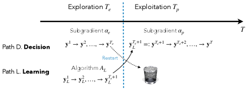
As discussed, a single first-order method may not simultaneously achieve good regret and accurate approximation of . However, this dilemma can be easily addressed if we decouple learning and decision-making and employ two first-order methods for learning and decision-making, respectively. The iteration cost of first-order methods is inexpensive, so it is feasible to maintain multiple of them to take the best of both worlds: the best possible learning algorithm and decision algorithm . Back to the exploration-exploitation framework, in the exploration phase, we can take to be the same subgradient method with constant stepsize, which we know at least guarantees performance for horizon length . The algorithm maintains two paths of dual sequences in the exploration phase, and when exploration is over, the solution learned by is handed over to the exploitation phase and adjusts stepsize based on the trade-off in Lemma 4.3. Since the subgradient methods with different stepsizes are used for decision-making in both exploration and exploitation, the actual effect of the framework is to restart the subgradient method. The final algorithm is presented in Algorithm 3 (Figure 1).
Decoupling learning and decision-making, Lemma 4.6 characterizes the performance of the whole framework.
Lemma 4.6.
Under the same assumptions as Lemma 4.3, the output of Algorithm 3 satisfies
and we have the following performance guarantee:
| (10) |
After balancing the trade-off by considering all the terms, we arrive at Theorem 4.1.
Theorem 4.1 (Main theorem).
Under the same assumptions as Lemma 4.6 and suppose is sufficiently large. If , then with
we have
In particular, if , there is no term. If , then with
we have
Theorem 4.1 shows that when the dual optimal set is a singleton, first-order methods can achieve regret using our framework. If , it is still possible to achieve better regret in terms of constant when . As a realization of our framework, we recover performance guarantees in the traditional setting of LP-based methods.
Corollary 4.1.
In the non-degenerate continuous support case, we get performance.
Corollary 4.2.
In the non-degenerate finite-support case, we get performance.
Again, the intuitions behind the algorithm are simple: error bound ensures is close to and allows online algorithm to localize in an neighborhood around ; exploration-exploitation allows us to learn from data and get close to ; decoupling learning and decision-making, we get the best of both worlds and control the regret in the exploration phase. These pieces together make first-order methods go beyond regret.
5 Numerical experiments
This section conducts experiments to illustrate the empirical performance of our framework. We consider both the continuous and finite support settings. To benchmark our algorithms, we compare
-
M1.
Benchmark subgradient method Algorithm 1 with constant stepsize .
-
M2.
Our framework Algorithm 3.
- MLP.
In the following, we provide the details of M2 for each setting.
-
•
For the continuous support setting, is the subgradient method with stepsize (Lemma 4.4). As suggested by Theorem 4.1, is the subgradient method with stepsize in the exploration phase . In the exploitation phase, takes stepsize . We always set and do not tune it through the experiments.
-
•
For the finite support setting, is ASSG [31] (Algorithm 4 in the appendix); is the subgradient method with stepsize in the exploration phase . In the exploitation phase, takes stepsize .
5.1 Continuous support
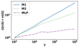
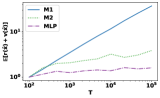
We generate from different continuous distributions. The performance of three algorithms is evaluated in terms of (which we will call regret for simplicity). We choose and 10 different evenly spaced over on -scale.
All the results are averaged over independent random trials.
For all the distributions, each is sampled i.i.d. from uniform distribution . The data is generated as follows: 1). The first distribution [18] takes and samples each i.i.d. from ; 2). The second distribution [19], takes , and samples each i.i.d. from ; 3).
The third distribution takes and samples from with and each i.i.d. from . 4).
The last distribution takes and samples and i.i.d. from and , respectively.
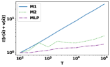
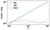
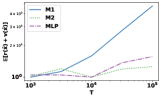
For each distribution and algorithm, we plot the growth behavior of regret with respect to . The performance statistics are normalized by the performance at . Figure 2 suggests that M2 has a better order of regret compared to M1, which is consistent with our theory. Although MLP achieves the best performance in , it requires significantly more computation time than M2, since it solves an LP for each . To demonstrate this empirically, we also compare the computation time of M1, M2, and MLP. We generate instances according to the first distribution with and . For each pair, we average the and computation time over independent trials and summarize the result in Table 2: MLP takes more than one hour when , whereas M2 only needs seconds and achieves significant better regret compared to MLP. Our proposed framework effectively balances efficiency and regret performance.
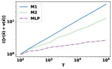
5.2 Finite support
We generate from different discrete distributions. The performance of three algorithms is evaluated in terms of . We choose and different evenly spaced over on log-scale. All the results are averaged over independent random trials. To generate a discrete distribution with support size , we first sample different from some distribution, then randomly generate a finite probability distribution over . At time , we sample with probability . We generate four discrete distributions as follows: 1). The first distribution takes and samples i.i.d. from and . Each is sampled from . 2). The second distribution takes and samples from the folded normal distribution with parameter and ; is sampled from the folded normal distribution with . Each element in is sampled from with . 3). The third distribution takes , and samples i.i.d. from exponential distribution ; is sampled from from . Each element in is sampled from , where . 4). The last distribution takes , and samples i.i.d. from and from with . Each element in is sampled from .
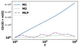
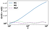
For each distribution and algorithm, we plot the normalized regret with respect to . Figure 3 indicates that M2 consistently outperforms M1 and exhibits regret. Moreover, M2 significantly reduces the computation time compared to MLP. To demonstrate this empirically, we also compare the computation time of M1, M2, and MLP. We generate instances according to the fourth distribution with and . For each pair, we average and computation time over independent trials and summarize the result in Table 3: MLP greatly reduces computation time compared to MLP but has comparable regret performance. First-order methods can replace LP-based methods in this case.
6 Conclusion
In this paper, we propose an online decision-making framework that allows first-order methods to achieve beyond regret. We identify that the error bound condition on the dual problem is sufficient for first-order methods to obtain improved regret and design an online learning framework to exploit this condition. We believe that our results provide important new insights for sequential decision-making problems.
References
- [1] Shipra Agrawal, Zizhuo Wang, and Yinyu Ye. A dynamic near-optimal algorithm for online linear programming. Operations Research, 62(4):876–890, 2014.
- [2] Alessandro Arlotto and Itai Gurvich. Uniformly bounded regret in the multisecretary problem. Stochastic Systems, 9(3):231–260, 2019.
- [3] Santiago R Balseiro, Omar Besbes, and Dana Pizarro. Survey of dynamic resource-constrained reward collection problems: Unified model and analysis. Operations Research, 2023.
- [4] Santiago R Balseiro, Haihao Lu, and Vahab Mirrokni. The best of many worlds: Dual mirror descent for online allocation problems. Operations Research, 2022.
- [5] Santiago R Balseiro, Haihao Lu, Vahab Mirrokni, and Balasubramanian Sivan. From online optimization to PID controllers: Mirror descent with momentum. arXiv preprint arXiv:2202.06152, 2022.
- [6] Dimitris Bertsimas and John N Tsitsiklis. Introduction to linear optimization, volume 6. Athena Scientific Belmont, MA, 1997.
- [7] Robert L Bray. Logarithmic regret in multisecretary and online linear programming problems with continuous valuations. arXiv e-prints, pages arXiv–1912, 2019.
- [8] James V Burke and Michael C Ferris. Weak sharp minima in mathematical programming. SIAM Journal on Control and Optimization, 31(5):1340–1359, 1993.
- [9] Guanting Chen, Xiaocheng Li, and Yinyu Ye. An improved analysis of lp-based control for revenue management. Operations Research, 2022.
- [10] Wenzhi Gao, Dongdong Ge, Chunlin Sun, and Yinyu Ye. Solving linear programs with fast online learning algorithms. In International Conference on Machine Learning, pages 10649–10675. PMLR, 2023.
- [11] Wenzhi Gao, Chunlin Sun, Chenyu Xue, and Yinyu Ye. Decoupling learning and decision-making: Breaking the barrier in online resource allocation with first-order methods. In International Conference on Machine Learning, pages 14859–14883. PMLR, 2024.
- [12] Hameed Hussain, Saif Ur Rehman Malik, Abdul Hameed, Samee Ullah Khan, Gage Bickler, Nasro Min-Allah, Muhammad Bilal Qureshi, Limin Zhang, Wang Yongji, Nasir Ghani, et al. A survey on resource allocation in high performance distributed computing systems. Parallel Computing, 39(11):709–736, 2013.
- [13] Jiashuo Jiang, Will Ma, and Jiawei Zhang. Degeneracy is OK: Logarithmic Regret for Network Revenue Management with Indiscrete Distributions. arXiv, 2022.
- [14] Patrick R Johnstone and Pierre Moulin. Faster subgradient methods for functions with hölderian growth. Mathematical Programming, 180(1):417–450, 2020.
- [15] Naoki Katoh and Toshihide Ibaraki. Resource allocation problems. Handbook of Combinatorial Optimization: Volume1–3, pages 905–1006, 1998.
- [16] Thomas Kesselheim, Andreas Tönnis, Klaus Radke, and Berthold Vöcking. Primal beats dual on online packing lps in the random-order model. In Proceedings of the forty-sixth annual ACM symposium on Theory of computing, pages 303–312, 2014.
- [17] Guokai Li, Zizhuo Wang, and Jingwei Zhang. Infrequent resolving algorithm for online linear programming. arXiv preprint arXiv:2408.00465, 2024.
- [18] Xiaocheng Li, Chunlin Sun, and Yinyu Ye. Simple and fast algorithm for binary integer and online linear programming. Advances in Neural Information Processing Systems, 33:9412–9421, 2020.
- [19] Xiaocheng Li and Yinyu Ye. Online linear programming: Dual convergence, new algorithms, and regret bounds. Operations Research, 70(5):2948–2966, 2022.
- [20] Zijian Liu and Zhengyuan Zhou. Revisiting the last-iterate convergence of stochastic gradient methods. arXiv preprint arXiv:2312.08531, 2023.
- [21] Alfonso Lobos, Paul Grigas, and Zheng Wen. Joint online learning and decision-making via dual mirror descent. In International Conference on Machine Learning, pages 7080–7089. PMLR, 2021.
- [22] Wanteng Ma, Ying Cao, Danny HK Tsang, and Dong Xia. Optimal regularized online allocation by adaptive re-solving. Operations Research, 2024.
- [23] Will Ma and David Simchi-Levi. Algorithms for online matching, assortment, and pricing with tight weight-dependent competitive ratios. Operations Research, 68(6):1787–1803, 2020.
- [24] Mohammad Mahdian, Hamid Nazerzadeh, and Amin Saberi. Online optimization with uncertain information. ACM Transactions on Algorithms (TALG), 8(1):1–29, 2012.
- [25] Vahab S Mirrokni, Shayan Oveis Gharan, and Morteza Zadimoghaddam. Simultaneous approximations for adversarial and stochastic online budgeted allocation. In Proceedings of the twenty-third annual ACM-SIAM symposium on Discrete Algorithms, pages 1690–1701. SIAM, 2012.
- [26] Alexander Rakhlin, Ohad Shamir, and Karthik Sridharan. Making gradient descent optimal for strongly convex stochastic optimization. arXiv preprint arXiv:1109.5647, 2011.
- [27] Jingruo Sun, Wenzhi Gao, Ellen Vitercik, and Yinyu Ye. Wait-less offline tuning and re-solving for online decision making. arXiv preprint arXiv:2412.09594, 2024.
- [28] Rui Sun, Xinshang Wang, and Zijie Zhou. Near-optimal primal-dual algorithms for quantity-based network revenue management. arXiv preprint arXiv:2011.06327, 2020.
- [29] Kalyan T Talluri, Garrett Van Ryzin, and Garrett Van Ryzin. The theory and practice of revenue management, volume 1. Springer, 2004.
- [30] Haoran Xu, Peter W Glynn, and Yinyu Ye. Online linear programming with batching. arXiv preprint arXiv:2408.00310, 2024.
- [31] Yi Xu, Qihang Lin, and Tianbao Yang. Stochastic convex optimization: Faster local growth implies faster global convergence. In International Conference on Machine Learning, pages 3821–3830. PMLR, 2017.
- [32] Tianbao Yang and Qihang Lin. RSG: Beating subgradient method without smoothness and strong convexity. The Journal of Machine Learning Research, 19(1):236–268, 2018.
Appendix
Appendix A Proof of Results in Section 3
A.1 Auxiliary results
Lemma A.1 (Hoeffding’s inequality).
Let be independent random variables such that almost surely. Then for all ,
Lemma A.2.
Consider standard form LP and suppose both primal and dual problems are non-degenerate. Then the primal LP solution is unique and there exists such that
for all primal feasible .
Proof.
Denote . Since both primal and dual problems are non-degenerate, is unique [6]. Denote to be the partition of basic and non-basic variables, and we have , where and . Similarly, denote to be the dual slack for , we can partition where and . We have by primal feasibility of . With dual feasibility, for some . Next, consider any feasible LP solution , and we can write
Since is non-degenerate, taking inverse on both sides gives and we deduce that
| (11) | ||||
| (12) | ||||
| (13) | ||||
| (14) |
where (11) uses , (12) plugs in , (13) plugs in and , (14) uses the fact that and . Re-arranging the terms,
| (15) |
On the other hand, we have
| (16) | ||||
| (17) |
Lemma A.3 (Learning algorithm for Hölder growth [31]).
Consider stochastic optimization problem with optimal set and suppose the following conditions hold:
-
1.
there exists some such that ,
-
2.
is a nonempty compact set,
-
3.
there exists some constant such that for all ,
-
4.
there exists some constant and such that for all
Then, there is a first-order method (Algorithm 4, Algorithm 1, 2, and 4 of [31]) that outputs after
iterations with probability at least .
Lemma A.4 (Last-iterate convergence of stochastic subgradient [20]).
Consider stochastic optimization problem . Suppose the following conditions hold:
-
1.
There exist such that
for all and ,
-
2.
It is possible to compute such that ,
-
3.
.
Then, the last iterate of the projected subgradient method with stepsize : satisfies
for all .
A.2 Dual learning algorithm
We include two algorithms in [31] that can exploit A4 and achieve the sample complexity in Lemma 3.1. Algorithm 4 is the baseline algorithm and Algorithm 5 is its parameter-free variant that adapts to unknown . Note that the algorithm has an explicit projection routine onto . According to [31], given parameters , Algorithm 4 is configured as follows:
A.3 Verification of the examples
A.3.1 Continuous support
The result is a direct application of Proposition 2 of [19].
A.3.2 Finite support
Denote to be the support of LP data associated with distribution . i.e., there are types of customers and customers of type arrive with probability . We can write the expected dual problem as
More compactly, we introduce slack and define . Then, the dual problem can be written as standard-form.
| (18) |
When , the result is an application of weak sharp minima to LP [8]. When the primal-dual problems are both non-degenerate, and applying Lemma A.2, we get the following error bound in terms of the LP optimal basis.
Lemma A.5.
Let denote the optimal basis partition for (18) and let denote the dual slack of primal variables , then
where . Moreover, we have .
Proof.
follows from Lemma A.2 applied to the compact LP formulation. Next, define where and . We deduce
and this completes the proof. ∎
A.3.3 General growth
Given , by optimality condition, and
where denotes the cdf. of the distribution of . Then we deduce that
Next, we invoke the assumptions and
| (19) | ||||
where (19) uses and that . Since for , this completes the proof.
A.4 Proof of Lemma 3.1
We verify the conditions in Lemma A.3.
Condition 1. Take . Then
where the first inequality holds since .
Condition 2 holds since , is closed and is a compact set.
Condition 3 holds since and . Hence .
Condition 4 holds by the dual error bound condition
with and .
Now invoke Lemma A.3 and we get that, after
iterations, the algorithm outputs such that with probability at least ,
and this completes the proof.
A.5 Proof of Lemma 3.2
We verify the conditions in Lemma A.4.
Condition 1. Since is convex and has Lipschitz constant , we take and deduce that
Condition 2 holds in the stochastic i.i.d. input setting.
A.6 Proof of Lemma 3.3
By definition and the fact that ,
According to A4, and
| (21) |
where (21) uses . Taking expectation and using , we arrive at
and it remains to bound . For any fixed ,
and for each , since ,
Using Lemma A.1,
Recall that by (4), and we construct an -net of as follows:
where we denote the centers of each net as and . In each member of the net, we have, by Lipschitz continuity of and , that
Next, with union bound,
Taking , we have
Taking gives
and
This completes the proof.
Appendix B Proof of results in Section 4
B.1 Auxiliary results
Lemma B.1 (Bounded dual solution [10]).
Assume that A1 to A3 hold and suppose Algorithm 1 with starts from and , then
| (22) |
almost surely. Moreover, if , then for all almost surely.
Proof.
Lemma B.2 (Subgradient method on strongly convex problems [26]).
Let and assume . Suppose is -strongly convex and . Then, the subgradient method with stepsize satisfies
with probability at least .
Lemma B.3 (Subgradient method for ).
Proof.
For any , we deduce that
| (23) | ||||
where (23) uses the non-expansiveness of the projection operator. Taking and using , we get
Since , we have, by convexity of , that
Next, we invoke A4 to get
Conditioned on history and taking expectation, we have
| (24) |
With , we have
Multiply both sides by and we get
| (25) | ||||
| (26) |
Re-arranging the terms, we arrive at
Taking expectation over all the randomness and telescoping from to , with (26) added, gives
and this completes the proof. ∎
Lemma B.4 (Subgradient with constant stepsize).
B.2 Proof of Lemma 4.1
By definition of regret, we deduce that
| (29) | ||||
| (30) | ||||
| (31) | ||||
| (32) | ||||
where (29) uses strong duality of LP; (30) uses the fact is a feasible solution and that is the optimal solution to the sample LP; (32) uses the definition of and that are i.i.d. generated. Then we have
| (33) | ||||
| (34) |
where (33) uses and (34) uses A2, A3. A simple re-arrangement gives
| (35) |
Next, we telescope the relation (35) from to and get
| (36) | ||||
| (37) | ||||
| (38) | ||||
| (39) |
B.3 Proof of Lemma 4.2
For constraint violation, recall that
and that
B.4 Proof of Lemma 4.3
Similar to the proof of Lemma 4.1 and Lemma 4.2, we deduce that
| (43) | ||||
where (43) is directly obtained from (31). Next, we analyze . Using (35),
and we deduce that
| (44) |
where (44) uses triangle inequality as in (38). Next, we consider constraint violation, and we have
| (45) |
where (45) is by and we bound
with the same argument as (42). Putting two relations together and using
We arrive at
| (46) |
where (46) uses
for all and it remains to analyze .
By Lemma 3.1, we have with probability that
Conditioned on the event , we deduce that
| (47) | ||||
| (48) |
where both (47) and (48) use the fact that imposed by Algorithm 2. Using Lemma 3.2, we have, conditioned on , that
| (49) | ||||
| (50) | ||||
| (51) | ||||
| (52) |
where (49) uses for nonnegative random variable ; (50) invokes Lemma 3.2; (51) uses and (52) plugs in (48). Putting the results together, we get
| (53) |
where (53) recursively applies and we arrive at
and this completes the proof. Here, the explicit expression of can be obtained from Lemma 3.1:
B.5 Proof of Lemma 4.4
Using Lemma B.2, it suffices to verify that the expected dual objective is strongly convex:
and indeed, is 1-strongly convex.
B.6 Proof of Lemma 4.5
First, we establish the update rule formula for in terms of . Specifically, we have
| (54) | ||||
| (55) | ||||
| (56) |
where (54) is obtained by the update rule of subgradient, (55) uses Jensen’s inequality, and (56) is obtained by the fact that is independent of and it is drawn uniformly from . Indeed, we have
Subtracting from both sides and multiplying both sides the the inequality by , we have
Next we condition on the value of and
| (57) |
Thus, given for some , we have
| (58) |
As a result, when , (58) implies
since we assume . This completes the proof.
B.7 Proof of Proposition 4.1
Based on [26], there exists some universal constant such that with probability no less than , for all , where and . Thus, without loss of generality, we assume
| (59) |
for all by setting a new random initialization and ignoring the all decision steps before the step. In the following, we show that SGM using stepsize must have regret or constraint violation for any initialization . We first calculate and similar to the proof of Lemma 4.5. Specifically, for , we have
which implies
| (60) |
Also, similarly, for we have under assumption (59)
which implies
| (61) |
Combining (60) and (61), we then can compute
| (62) | ||||
| (63) | ||||
In addition, since , by Lemma A.1, we have with probability no less than
Consequently, by (62), we have
| (64) |
This is the summation of constraint violation and constraint (resource) leftover, and thus, the summation of constraint violation and the regret must be no less than .
B.8 Proof of Theorem 4.1
First note that for sufficiently large , the condition from Lemma B.1 will be satisfied and all the dual iterates will stay in almost surely. When , we consider
Since only appears in , we let to optimize the trade-off. Hence, it suffices to consider
Taking and with , we have according to Lemma 3.1 and (8), and . Moreover, we have, using to denote equivalence under notation, that
Suppose . Then and
| (65) |
where (65) uses and that . To find the optimal trade-off, we solve the following optimization problem
| subject to |
The solution yields and and
always holds. Hence
and this completes the proof for .
Next, consider the case . In this case we need to consider the trade-off:
Note that and that make it impossible to achieve better than regret. Hence, we consider improving the constant associated with .
Using and suppose are of the same order with respect to ,
Suppose we take and for and we let . Then, and
Hence, it suffices to consider
Taking and to optimize the two trade-offs, we get
With , we have
Since , this completes the proof.
B.9 Removing additional when
When , the dual error bound condition reduces to quadratic growth, and it is possible to remove the factor in the regret result. Recall that terms appear when bounding and . For , using a tailored analysis, Lemma B.3 guarantees
Moreover, using Lemma B.4, we can directly bound the expectation
Therefore, terms can be removed from the analysis.
B.10 Learning with unknown parameters
It is possible that and are unknown in practice. When is unknown, it is possible to run parameter-variants of first-order methods Algorithm 5, which is slightly more complicated. In terms of , in the finite-support setting, the LP polyhedral error bound always guarantees . In the continuous support setting, it suffices to know an upperbound bound on : if A4 holds for some , then given ,
and A4 also holds for .