Bi-fidelity Modeling of Uncertain and Partially Unknown Systems Using DeepONets
Abstract
Recent advances in modeling large-scale, complex physical systems have shifted research focuses towards data-driven techniques. However, generating datasets by simulating complex systems can require significant computational resources. Similarly, acquiring experimental datasets can prove difficult. For these systems, often computationally inexpensive, but in general inaccurate models, known as the low-fidelity models, are available. In this paper, we propose a bi-fidelity modeling approach for complex physical systems, where we model the discrepancy between the true system’s response and a low-fidelity response in the presence of a small training dataset from the true system’s response using a deep operator network (DeepONet), a neural network architecture suitable for approximating nonlinear operators. We apply the approach to systems that have parametric uncertainty and are partially unknown. Three numerical examples are used to show the efficacy of the proposed approach to model uncertain and partially unknown physical systems.
Keywords Bi-fidelity method Uncertain system Neural network Deep Operator Network Uncertainty quantification
1 Introduction
The ubiquitous presence of uncertainty often affects the modeling of a physical system using differential equations. For example, in engineering systems, the sources of uncertainty can include material properties, geometry, or loading conditions. This type of uncertainty is known as parametric uncertainty and differs from one realization to another. In contrast, during modeling, some physical phenomena are often ignored or simplified, which leads to the so called structural uncertainty [1]. Both types of uncertainties can be present in a real-life engineering system, and should be addressed when developing digital twins of the system. Models developed using polynomial chaos expansion [2, 3], Gaussian process regression [4, 5], and other response surfaces [6, 7, 8] address parametric uncertainty, which defines possible realizations of the system. However, the cost of developing these models increases significantly with the dimension of the uncertain variables [9].
Neural networks, commonly used in computer vision [10] and pattern recognition problems [11], have been used to model physical systems in the presence of uncertainty [12, 13]. To model physical systems, Raissi et al. [14] augmented the standard data discrepancy loss with the residual of the corresponding governing equations. This approach was termed "Physics-informed neural networks." Subsequently, a significant amount of work employing this approach to address basic computational mechanics problems came into prominence in the literature, some notable ones being Karniadakis et al. [15], Cai et al. [16], and Viana and Subramaniyan [17]. Among these several works address the parameteric uncertainty in the system [18, 19, 20, 21, 22, 23]. However, machine learning studies that address structural uncertainty in modeling are scarce. Among them, Blasketh et al. [24] used neural networks combined with governing equations to address modeling and discretization errors. Zhang et al. [25] used the physics-informed approach to quantify both the parametric and approximation uncertainty of the neural network. Duraisamy and his colleagues further trained neural networks to comprehend the discrepancies between turbulence model prediction and the available data [26, 27, 28].
Recently, several neural network architectures capable of approximating mesh-independent solution operators for the governing equations of physical systems have been proposed [29, 30, 31, 32, 33, 34, 35], drawing inspiration from the universal approximation theorem for operators in Chen and Chen [36]. These architectures overcome two shortcomings of the physics-informed use of neural networks to learn a system’s behavior: firstly, they do not depend on the mesh used to generate the training dataset. Secondly, they are solely data-driven and do not require the knowledge of the governing equations. Among these network architectures, the deep operator network (DeepONet) proposed in Lu et al. [29, 34] uses two separate networks — one with the external source term as input and the other with the coordinates where the system response is sought as input. The former network is known as the branch network while the latter is known as the trunk network. Outputs from these two networks are then used in a linear regression model to produce the system response. Lu et al. [37] showed how the computational domain can be decomposed into many small subdomains to learn the governing equation with only one solution of the equation. While Cai et al. [38] used DeepONets for a multiphysics problem involving modeling of field variables across multiple scales., Ranade et al. [39] and Priyadarshini et al. [40] employed DeepONets for approximating joint subgrid probability density function in turbulent combustion problems and to model non-equilibrium flow physics respectively. Additionally, Wang et al. [41, 42] used the error in satisfying the governing equations to train the DeepONets, with a variational formulation of the governing equations being applied by Goswami et al. [43] to train DeepONets to model brittle fracture. Further comparisons of DeepONet with the iterative neural operator architecture proposed in Li et al. [32] were performed in Kovachki et al. [44] and Lu et al. [45]. The approximation errors in the latter neural operator architectures were subsequently discussed in Kovachki et al. [46], Lanthaler et al. [47], Deng et al. [48], and Marcati and Schwab [49].
The training datasets required to construct the DeepONets for a complex physical system can often be limited due to the computational burden associated with simulating such systems. Similarly, repeating experiments to obtain measurement data can become infeasible. In the presence of a small dataset from the true high-fidelity system, we propose herein a modeling strategy with DeepONets that uses a similar but computationally inexpensive model, known as low-fidelity, that captures many aspects of the true system’s behavior. The discrepancy between the response from the true physical system and the low-fidelity model is estimated using DeepONets. The assumption used here is that the modeling of the discrepancy requires only a small training dataset of the true system’s response, and as a result, bi-fidelity approaches are often advantageous with scarce training data from the high-fidelity simulations [50, 51, 52]. In principle, we train a DeepONet that uses the low-fidelity response as the input of the branch network to predict the discrepancy between the low- and high-fidelity data. However, we do not incorporate physics loss or error in satisfying the governing equations (as previously employed in physics informed neural networks) to circumvent potential bias incorporation in partially known engineering systems subject to the presence of structural uncertainty.
In this paper, we employ three numerical examples to show the efficacy of the proposed bi-fidelity approach to modeling the response of an uncertain and partially unknown physical system. The first two examples consider a nonlinear oscillator and a heat transfer problem, respectively, where uncertainty is present in some of the parameters of the governing equations. The low-fidelity model used in these examples ignores the nonlinearity or some of the uncertain components of the governing equations. In the third example, we model power generated in a wind farm, , with the two and three dimensional simulations respectively serving as high and low-fidelity model systems.
The rest of the paper is organized as follows: first, we provide a brief background on DeepONets in Section 2. Then, we present our proposed approach for modeling the discrepancy between a low-fidelity system response and the true response for uncertain and partially unknown systems in Section 3. Three numerical examples involving a dynamical system, a heat transfer problem, and a wind farm application are subsequently used in Section 4 to showcase the efficacy of the proposed approach. Finally, we conclude the paper with a brief discussion on future applications of the proposed approach.
2 Background on DeepONets
Let us assume the governing equation of a physical system in a domain is given by
| (1) |
where is a nonlinear differential operator; is the location; is the response of the system; and is the external source. For a boundary value problem, Dirichlet boundary condition on and/or Neumann boundary condition on are also present, where is the differential operator for the Neumann boundary condition; with the boundary of the domain being ; and . For an initial value problem, an initial condition is used instead, where is the initial instant. The solution of (1) is given by , where denotes the solution operator. For and , there exist embeddings and .
The DeepONet architecture proposed in Lu et al. [29] approximates the solution operator as
| (2) |
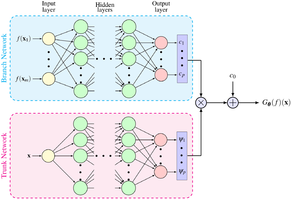
where is a constant bias parameter; are obtained from a neural network, known as the branch network, that has the input function (e.g., external source term) measured at locations as input; are obtained from a neural network, known as the trunk network, that has the location as the input; and is the parameter vector containing weights and biases and from the branch and trunk networks, respectively, and . This approximation is based on the universal approximation theorem in Chen and Chen [36] for operators. A schematic of the DeepONet architecture used in this study is shown in Figure 1. The main advantage of using a DeepONet architecture over other standard ones, such as feedforward, recurrent, etc., is that DeepONet provides a mesh-independent approximation of the solution operator since DeepONet uses a set of parameters trained only once with different mesh discretizations [32, 29].
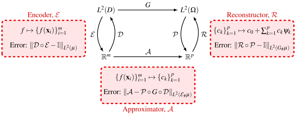
Lanthaler et al. [47] showed that the DeepONet can be thought of as a composition of three components. The first component is an encoder that maps the input function space to sensor inputs for . The second component, the approximator , models the relation between sensor inputs and the coefficients . The encoder and the approximator together comprise the branch network. The third or the final component of DeepONet is the reconstructor, which maps the output of the branch network to the response , thereby showing dependence on the trunk network outputs . With approximate inverses of the encoder and reconstructor defined as decoder and projector , respectively, three errors associated with DeepONet approximation can be defined as encoding error , approximation error , and reconstruction error , where is an identity matrix; is the measure associated with ; and are push-forward measures associated with the encoder and operator , respectively. Figure 2 shows the three components of a DeepONet and associated errors as defined here. The total approximation error associated with a DeepONet depends on these three errors as outlined in Theorem 3.2 in Lanthaler et al. [47].
The parameter vector is estimated by solving the optimization problem
| (3) |
where in the training dataset for each of realizations of the external source term , measurements of the response at locations , which might not be the same as the locations where the external source term is measured, are used. These sensor locations can be random or equispaced inside the domain and kept fixed during training. The optimization problem in (3) can be solved using stochastic gradient descent [53, 54, 55] to obtain optimal parameter values of the DeepONets. In this paper, we use a popular variant of stochastic gradient descent, known as the Adam algorithm [56], to train DeepONets. Note that in Lu et al. [29], the input function is sampled from function spaces with the locations as domain and the external source as range, such as Gaussian random field and Chebyshev polynomials. However, for practical reasons, in this paper, we use probability distribution of the uncertain variables associated with the problems to sample the input function. However, the number of training data for DeepONets can be limited if the computational cost of the simulation of the physical system or the cost of repeating the experiments is significant. In this study, to address the challenge of training DeepONets in the presence of limited data, we propose a bi-fidelity training approach utilizing a computationally inexpensive low-fidelity model of the physical system. In the next section, we detail this proposed approach and discuss two applications to address parametric and structural uncertainties present in the system.
3 Methodology
In the present work, we assume a low-fidelity model of the physical system in (1) is given by
| (4) |
where is the low-fidelity response; is the differential operator related to the low-fidelity model; and is the external source in the low-fidelity model. Next, we denote the discrepancy between the solution of the low-fidelity model and that of the physical system as
| (5) |
As it is often the case that the low-fidelity model will capture many important aspects of the physical system’s response, we assume that the training of a DeepONet for modeling is easier than modeling the true response and that generating the low-fidelity response is computationally inexpensive. We present two applications of the proposed approach next. Note that is estimated from the DeepONet and from the low-fidelity model for any new to predict the response . Further, this new location need not be the same locations used during training or the places where the external source is measured due to the use of DeepONet to model . We also do not use another DeepONet or neural network to model the low-fidelity response as the simulation of the low-fidelity model is computationally inexpensive, and this avoids any approximation error introduced through a low-fidelity trained network.
3.1 Application I: Systems with Parametric Uncertainty
The proposed approach can be used for modeling systems with parametric uncertainty, where a computationally inexpensive low-fidelity model of a similar system is available. For example, consider a system described by
| (6) |
where is the vector of uncertain variables; and are deterministic and uncertain (or stochastic) parts of the differential operator in (1), respectively; the response depends on the uncertain variables ; and the external source may depend on as well. In this case, a low-fidelity model for (6) can be defined as follows
| (7) |
Hence, the response of the physical system is approximated as
| (8) |
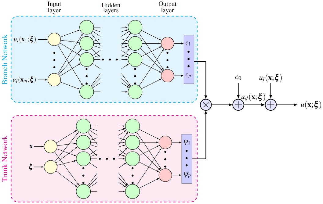
where are used as the input of the branch network and as the input of the trunk network to model the discrepancy . A schematic of the approximation in (8) is shown in Figure 3.
As a special case, when the operators and are linear, using (5) in (6) we arrive at
| (9) |
which is modeled using a DeepONet, where is the solution to (7) and . Note that we do not necessarily require the linearity of the differential operators for the proposed approach to apply. However, we make that assumption to illustrate the simplified construction of the low-fidelity model and the correction.
3.2 Application II: Systems with Structural Uncertainty
In this application, we propose to use (5) to model the response of a partially unknown system. For example, let us assume we can rewrite (1) as follows
| (10) |
where and are the known and unknown parts of the differential operator, respectively; and and are the known and unknown parts of the external source, respectively. A low-fidelity model for this application can be defined as
| (11) |
The response of the physical system is approximated next as
| (12) |
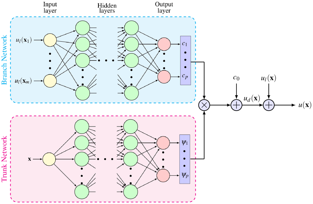
where we use as the branch network input and as the trunk network input. Figure 4 shows a schematic of the approximation in (12).
As a special case, assuming the differential operators and are linear leads to the following relation for in (5)
| (13) |
As before, we do not necessarily require linear differential operators to apply the proposed method. Note that it is straightforward to apply the proposed approach for an uncertain and partially unknown system using as trunk network input, as in the previous subsection and addresses both parametric and structural uncertainties. Also, the low-fidelity model can be uncertain in these two applications, but for brevity we do not explicitly write the dependence of the low-fidelity solution on in this section.
3.3 Choice of Low-fidelity Model
The choice of the low-fidelity model can have a significant effect on the total DeepONet approximation error. As discussed in Section 2, with a three-component decomposition of the DeepONet, Lanthaler et al. [47] showed that the total error in a DeepONet approximation depends on errors in each of these components [47, Eq. (3.4)]. Among them, the error in the approximator depends on the neural network approximation error, such as in Yarotsky [57, Thm. 1]. On the other hand, the errors in encoder and reconstructor depend on the eigenvalues of covariance operator of the branch network inputs and [47], respectively. In particular, these errors can be bounded from below using , where are eigenvalues of the covariance operator of the branch network input for encoding error and eigenvalues of the covariance operator of for reconstruction error , respectively.
In the bi-fidelity DeepONet, we are replacing the external source term with the low-fidelity response in the branch network input, and the discrepancy is modeled using the DeepONet. Hence, an ideal choice for the low-fidelity model that will reduce the encoding error will be a low-pass filter system that will remove most of the eigenvalues for of the covariance operator of the branch network input. Also, in many cases, encoding the low-fidelity model’s response will be easier than encoding the external source reducing the encoding error. Similarly, to reduce the reconstruction error , we can select a low-fidelity model such that the eigenvalues of covariance of has smaller magnitudes for . However, in practice, we may be limited in terms of choosing the low-fidelity model. A simplified physics or a coarser discretization is often used as the low-fidelity model in most of the multi-fidelity methods. In our numerical examples described in Section 4, we will show that these practical low-fidelity models can still provide significant improvements in the total DeepONet approximation error.
As an elementary example to illustrate the above discussion, we consider a duffing oscillator with governing differential equation
| (14) |
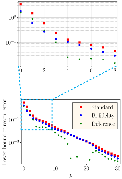
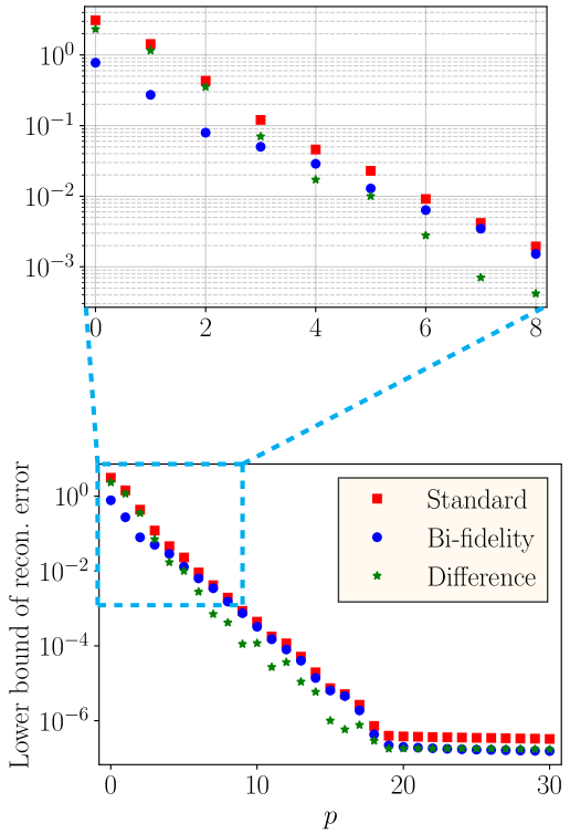
where is the damping coefficient; is the linear stiffness coefficient; is the nonlinear stiffness coefficient; is the amplitude of the external force; is the frequency of the external force; and is the initial response of the system. We consider the two applications of bi-fidelity DeepONet discussed in Section 3. In the first application, the parameters and are assumed as uncertain, and a low-fidelity model that does not include the term is considered. For this case, Figure 5(a) shows the lower bound of the reconstruction error computed using , where are eigenvalues of the sample covariance matrix of estimated using 2000 realizations of the random parameters [47, Th. 3.4]. In the second application, we use a low-fidelity model that does not consider the term and is replaced with a different . The lower bound of the reconstruction error computed similarly for this case is shown in Figure 5(b). These two plots show that for smaller in (2), the bi-fidelity DeepONet provides significantly lower bound for the reconstruction error. For large , this lower bound for both bi-fidelity DeepONet and the DeepONet described in Section 2, denoted as standard in the rest of the paper, reaches zero.
Experimental results for these two applications of bi-fidelity DeepONet are provided in the next section. Note that, we can also choose different low-fidelity models that do not necessarily provide a smaller lower bound for the reconstruction error, but the approximation and encoding errors are smaller with bi-fidelity DeepONet compared to a standard DeepONet as is done in Example 4.2.
4 Numerical Examples
In this section, we illustrate the proposed approach in approximating the discrepancy between the low-fidelity response and the physical system’s response with DeepONets using three numerical examples. The first example uses nonlinear ordinary differential equation for an initial value problem. In the second example, we model a nonlinear heat transfer in a thin plate, where a partial differential equation for the boundary problem is used. We consider both parametric and structural uncertainties to illustrate the applications I and II of the proposed approach from Section 3 in these two examples. The third example considers flow through a wind farm with a combination of parametric and structural uncertainties, where two-dimensional and three-dimensional simulations are used as the low- and high-fidelity model of the system, respectively. In these examples, we use two separate datasets, namely a training dataset and a validation dataset . We use the training dataset to train the DeepONets, and the accuracy of the trained DeepONets is measured using the validation dataset , with the relative validation root mean squared error (RMSE), , defined as follows
| (15) |
where is the -norm of its argument, is the vector of predicted response using DeepONets, and is from the validation dataset . Note that we select the number of hidden layers in the trunk and branch networks and the number of neurons per hidden layer using an iterative procedure, where we increase the number of neurons per hidden layer gradually up to an upper limit (100 in this study) and then add hidden layers to the network until we observe no reduction of . For the number of terms in (8) and (12), we increase in multiples of 10 to a maximum, which is the number of neurons in the hidden layers, to observe any reduction of .
4.1 Example 1: Duffing Oscillator
In this example, we use a duffing oscillator described by the governing differential equation (14). We use a neural network that has three hidden layers with 40 neurons each as the branch network and a neural network that has two hidden layers with 40 neurons each as the trunk network. We use ELU as the activation function in these networks [58]. The number of terms in the summation in (2) is fixed at following the procedure discussed in the previous section.
4.1.1 Application I: Parametric Uncertainty
For the oscillator defined in (14), we use , , and . The uncertain variables are assumed as with and , where denotes a uniform distribution between limits and . We use a training dataset with and a validation dataset with realizations of the uncertain variables uniformly sampled from their corresponding distributions, respectively, where the response is measured at 100 equidistant points along . A low-fidelity model of the system can be specified without the nonlinear stiffness, as follows
| (16) |
where is the low-fidelity response. Note that uncertainty in the low-fidelity model only comes through the uncertain variable . Figure 6(a) depicts a representative realization of , the low-fidelity response , and the discrepancy . Note that in this example the cost of generating the low- and high-fidelity datasets is insignificant.
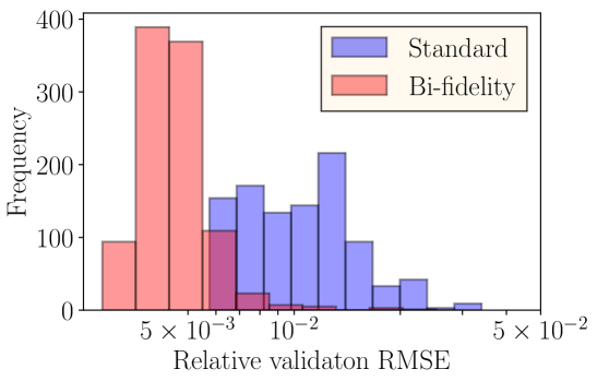
The proposed use of DeepONet to model the discrepancy between the low-fidelity and the true responses produces as the validation error with the validation dataset . In contrast, the standard DeepONet results in a validation error of . Figure 6(b) compares the histograms of the relative validation RMSE of these two approaches. Hence, in this case, the proposed approach improves the validation error by more than a factor of two, as modeling of the discrepancy proved to be easier using the same DeepONet architecture than modeling the response .
4.1.2 Application II: Partially Unknown System (Structural Uncertainty)
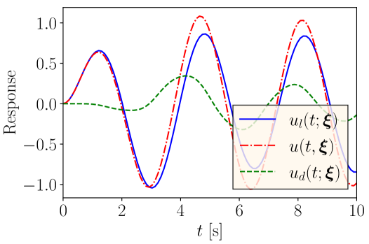
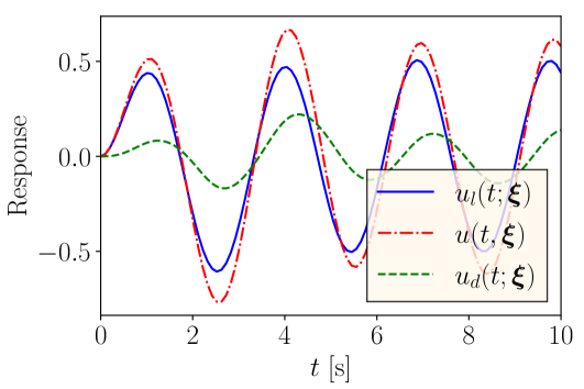
In this case, we assume , , and as before, but . The frequency of the external load is assumed to be uniformly distributed as before. We use a training dataset with , where we also add 5% additive Gaussian white noise to the dataset, and a validation dataset with . The low-fidelity model is assumed as
| (17) |
where the nominal value of the damping coefficient is . Hence, the unknown dynamics not modeled in the low-fidelity model can be given by
| (18) |
Figure 7(a) shows a comparison of the response from the low-fidelity model , true response , and their difference . When DeepONet is used to model the discrepancy between the true response and the low-fidelity model response, it produces a validation error of . Note that the standard use of DeepONet produces an of with the same training and validation datasets. Figure 7(b) shows a comparison of histograms from the proposed use of DeepONet to model and the standard use of DeepONet as described in Section 2. The figure shows that, in this case as well, modeling as a function of the low-fidelity response using DeepONet can achieve better accuracy compared to the standard use. Hence, this example shows the effectiveness of the proposed approach to model the discrepancy using DeepONet for uncertain and partially unknown dynamical systems, which reduces the validation error by a factor of more than two.
4.2 Example 2: Nonlinear Steady-state Heat Transfer in a Thin Plate
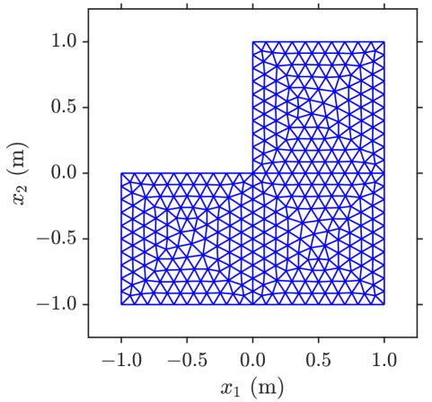
In our second example, we use a two-dimensional steady-state heat transfer problem in a thin L-shaped plate with dimensions shown in Figure 8(a). The left boundary is assumed to have a constant temperature of K. The steady-state temperature at any location inside the plate, , is given by
| (19) |
where ; is the thickness of the plate; is the thermal conductivity of the plate; is the amount of heat transferred through one face of the plate per unit area using convection; is the amount of heat transferred through one face of the plate per unit area using radiation; and is the amount of heat added to the plate per unit area from an internal heat source. Heat transferred by convection can be given by Newton’s law of cooling as
| (20) |
where is the specified convection coefficient and is the ambient temperature. For heat transferred due to radiation, the Stefan-Boltzmann law can be used,
| (21) |
where is the emissivity of the plate surface and is the Stefan-Boltzmann constant of the plate. Given (20) and (21), we rewrite (19) as
| (22) |
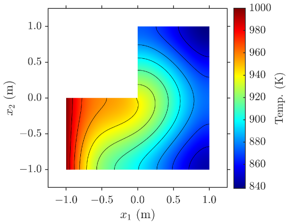
In this example, we set m; ; ; and (similar to copper) to generate the datasets. We also assume the internal heat source to be an uncertain squared exponential source centered at the corner given by
| (23) |
where and is a standard Gaussian random variable. We use the finite element method with the mesh shown in Figure 8(a) to solve (22). Figure 8(b) shows a realization of the steady-state temperature in the plate. In this example, we use a neural network that has three hidden layers with 40 neurons each and ELU activation as the branch network, and a neural network that has two hidden layers with 40 neurons each and ELU activation as the trunk network. The number of terms in the summation in (2) is fixed at to produced the smallest validation error.
4.2.1 Application I: Uncertain Thermal Conductivity
In our first application, we model the thermal conductivity as
| (24) |
where and is a zero mean Gaussian random field with a square exponential covariance function
| (25) |
where are length scale parameters, which we choose as for both dimensions. A Karhunen-Loève (KL) expansion truncated at the 25th term that captures 97% of the energy (defined as the sum of all eigenvalues) is used to generate realizations of the random field . For the low-fidelity model, we consider
| (26) |
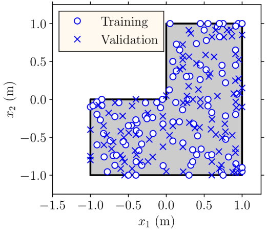
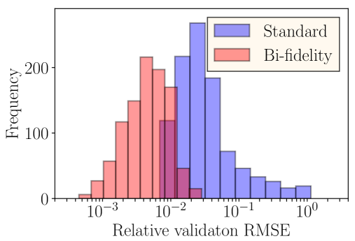
where is the temperature given by the low-fidelity model; and . Hence, the low-fidelity model is deterministic and we only need to solve it once. Here, the input to the trunk network of the bi-fidelity DeepONet that models the discrepancy (see Figure 3) contains 25 standard normal random variables used in the KL expansion of , in (23), and the location for predicting the temperature. We use realizations of the uncertain variables in the training dataset and realizations for the validation dataset . For each of these realizations, we measure the temperature of the plate at 200 locations marked using circles and crosses in Figure 9(a). During training, we use the temperature at 100 of these locations marked with circles and validate the DeepONets by predicting the temperature at the remaining 100 locations marked with crosses. We compare the result to the standard use of DeepONet as discussed in Section 2, where a sample of and the right hand side of (22), measured at the training locations, marked with circles in Figure 9(a), are used as input to the branch network.
Using the bi-fidelity DeepONet, the validation error , as defined in (15), is . However, the validation error in the standard use of DeepONet is . Figure 9(b) shows the histograms comparing the errors from these two approaches, denoted as ‘standard’ and ‘bi-fidelity’, respectively. The validation error and the histograms show that the proposed approach improves the accuracy of the predictions by almost an order of magnitude. This is primarily due to the fact that modeling of the temperature discrepancy can be performed relatively accurately using DeepONets in the presence of a small training dataset.
4.2.2 Application II: Partially Unknown System (Structural Uncertainty)
Next, we assume that the low-fidelity model is unaware of the radiation component in (22), i.e.,
| (27) |
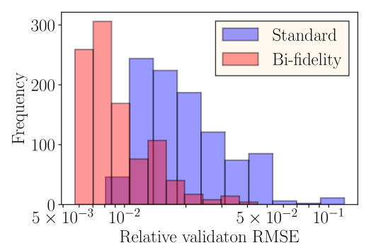
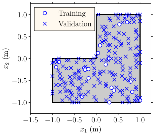
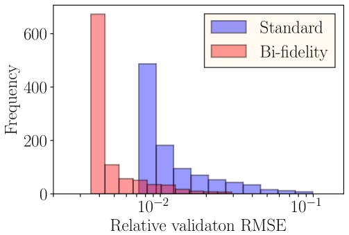
where is used. Hence, the low-fidelity model is deterministic and we only need to solve it once. Here, we use and as the input to the trunk network. The training dataset and the validation dataset consist of and data points, respectively, similar to the previous subsection. For each of these realizations, we measure the temperature of the plate at 200 locations marked using circles and crosses in Figure 10(a). During training, we use the temperature at 20 of these locations marked with circles and validate the DeepONets by predicting the temperature at the remaining 180 locations marked with crosses. When using DeepONet for modeling the discrepancy between the low-fidelity model and the true system, the validation error is . The standard use of DeepONet, however, gives as , one order of magnitude larger than the proposed bi-fidelity DeepONet. Figure 10(b) compares the histograms of the errors from these two approaches, illustrating the advantage of the bi-fidelity approach.
4.3 Example 3: Wind Farm
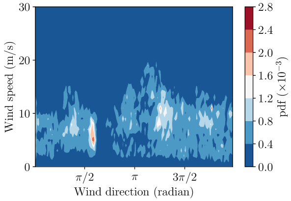
In our third example, we model the power generated in a wind farm and consider uncertain wind speed, inflow direction, and yaw angle. Estimating the expected power with respect to the joint distribution of wind speed and direction is a common calculation in determining the annual energy production of a wind plant; however, the number of function evaluations required often precludes the use of high-fidelity models in industry [59]. Deliberately, yawing wind turbine rotors out of perpendicular to incoming wind is an emerging flow control technique called wake steering, which can improve the overall plant output by directing wind turbine wakes away from downwind turbines [60]. The wake steering optimization problem is fraught with uncertainty due to misalignment in the nacelle-mounted wind vanes located just downwind of the rotor [61]. We consider two layouts of a wind farm with the number of turbines six and 64, respectively. For the probability distribution of uncertain wind speed and direction, we use 10 minute-average measurement data from the Princess Amalia wind farm in the Netherlands. The joint probability density function of the wind speed and direction estimated using these measurements is shown in Figure 11.
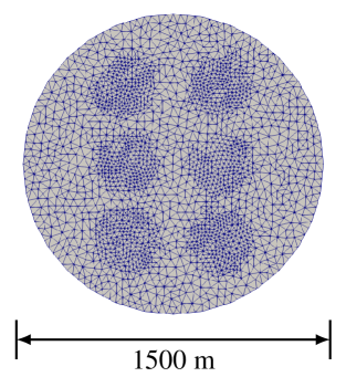
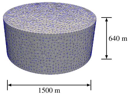
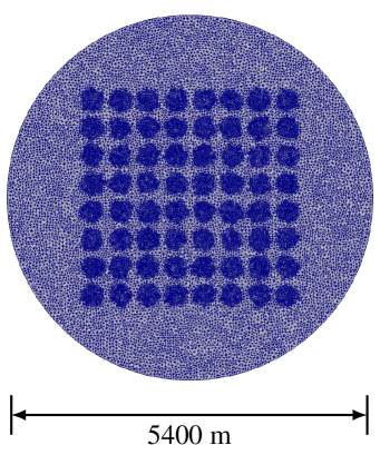
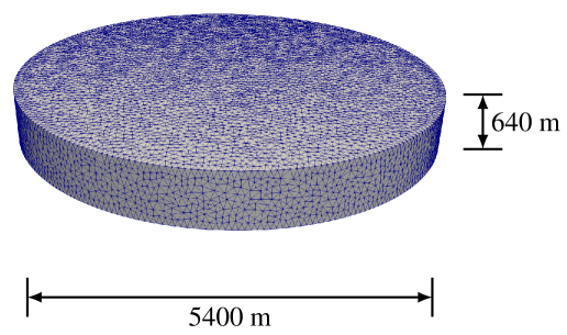
For each realization of the wind speed, direction, and yaw angle, we use the WindSE toolkit [62], a Python package with FEniCS [63] as the backend solver, to generate the training and validation datasets. Two-dimensional (2D) Reynolds Averaged Navier-Stokes (RANS) simulations using the finite element mesh shown in Figure 13(a) are used to generate the low-fidelity data. Three-dimensional (3D) simulations using the mesh shown in Figure 13(b) are used to estimate the power generated from the true system. For the two- and three-dimensional simulations, a mixing length model [64][65, 7.1.7] is used for closing the turbulent stress term, with a uniform mixing length m. In the three-dimensional simulations, a velocity log-profile is used for the atmospheric boundary layer with Von-Karman constant . The log profile is such that the hub-height velocity is the value of the sample drawn from the pdf shown in Fig. 11. In the two-dimensional simulations, the governing equations follow the 2D approximation of Boersma et al. [66] to approximate the flow field at hub-height, which is sufficient for estimating the power output.
We use a training and validation datasets consisting of and realizations of the uncertain variables and power generated. The realizations of wind speed and wind direction are generated using the histograms from the dataset for the Princess Amalia wind farm in the Netherlands. We use a neural network with three hidden layers and 100 neurons each with ELU activation as the branch network and another neural network with two hidden layers and 100 neurons each with ELU activation as the trunk network in this example. In (2), we truncate the summation at that produces the smallest validation error. Results for two layouts with six and 64 turbines are discussed next.
4.3.1 Layout 1: Six Turbines
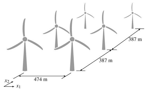
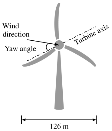
First, we model the power generated in a wind farm with six turbines arranged in a grid as shown in Figure 12(a). The wind turbines are placed 474 m apart in the direction and 387 m apart in the direction. We use the NREL 5 MW reference turbine [67], which has a 126 m rotor diameter and 90 m hub height. Figure 12(b) shows a single turbine with yaw angle between the wind direction and the turbine axis, which is used as an input parameter in this example.
We consider three cases here. In Case I, we only consider wind speed and direction as uncertain variables and assume yaw angle to be zero for all the turbines. In Case II, we assume the yaw angle to be uncertain and uniformly distributed between , but the same for all the turbines. In the final Case III, we assume each of the six turbines has uncertain yaw angles that are independent and identically distributed uniformly between .
We compare the the results with a standard DeepONet that uses wind speed, direction, and yaw angle (for the last two cases) as branch network input and the turbine location as the trunk network input. Note that one 2D simulation of this layout takes 4.69 s (average of 1000 runs) compared to 3.54 min (average of 1000 runs) for one 3D simulation on the National Renewable Energy Laboratory’s Eagle high-performance computing system (https://www.nrel.gov/hpc/eagle-system.html). Therefore, for a fair comparison, we train this DeepONet with a training dataset consisting of 103 realizations of the uncertain variables and corresponding power generated (i.e., with similar computational cost of generating the training dataset compared to the bi-fidelity training dataset used in the proposed approach).
We list the results in Table 1, which shows that the proposed use of DeepONet to model the discrepancy between the power outputs from 2D and 3D simulations provides significant improvement in the validation error. Also, the standard use of DeepONet shows improvement when we add yaw angle as another random input. This is primarily due to the fact that yaw angle has a significant effect on the power generated, and the standard DeepONet is able to model that relation with increasing connection due to the addition of a new input node in the network. A similar but slight improvement in the proposed approach can also be noticed in Cases II and III in Table 1.
| Case | Method | Network input | Histograms of validation error | ||
| Branch | Trunk | ||||
| I | Standard | ![[Uncaptioned image]](https://cdn.awesomepapers.org/papers/62495185-4474-4e6a-8cdc-f4970a0a5a24/x22.png) |
|||
| Wind speed, | Turbine | ||||
| wind direction | location | ||||
| Bi-fidelity | |||||
| Power | Wind speed, | ||||
| generated | wind direction, | ||||
| from | turbine location | ||||
| 2D simulations | |||||
| II | Standard | ![[Uncaptioned image]](https://cdn.awesomepapers.org/papers/62495185-4474-4e6a-8cdc-f4970a0a5a24/x23.png) |
|||
| Wind speed, | |||||
| wind direction, | Turbine | ||||
| yaw angle | location | ||||
| Bi-fidelity | |||||
| Power | Wind speed, | ||||
| generated | wind direction, | ||||
| from | yaw angle, | ||||
| 2D simulations | turbine location | ||||
| III | Standard | ![[Uncaptioned image]](https://cdn.awesomepapers.org/papers/62495185-4474-4e6a-8cdc-f4970a0a5a24/x24.png) |
|||
| Wind speed, | |||||
| wind direction, | Turbine | ||||
| individual | location | ||||
| yaw angle | |||||
| Bi-fidelity | |||||
| Power | Wind speed, | ||||
| generated | wind direction, | ||||
| from | individual yaw angle, | ||||
| 2D simulations | turbine location | ||||
4.3.2 Layout 2: 64 Turbines
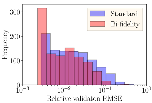
In this layout, we consider 64 turbines in total arranged in a grid that is more characteristic of the size of a utility-scale wind plant. Other specifications of the turbine layout and the input parameters are the same as before. Figure 14 shows the two- and three-dimensional meshes used to generate the training and validation datasets. The results from the proposed bi-fidelity training of DeepONets are compared with a DeepONet (denoted as ‘standard’) trained only using a high-fidelity dataset with wind speed, direction, and yaw angle as branch network inputs and the turbine location as the trunk network input. Note that one 2D simulation of this layout takes 3.68 min. (average of 300 runs) compared to 1.15 hrs. (average of 300 runs) for one 3D simulation on the National Renewable Energy Laboratory’s Eagle high-performance computing system. As before, for a fair comparison, we train the standard DeepONet with a training dataset consisting of 106 realizations of the uncertain variables and generated power to keep the cost of generating the training dataset similar to that of the bi-fidelity DeepONet. In this layout, the validation error using the proposed approach is , which is about half of , obtained using the standard DeepONet. Figure 15 shows the histograms of the validation errors.
5 Conclusions
In this paper, we propose a bi-fidelity approach for modeling uncertain and partially unknown system responses using DeepONets. In this approach, we utilize a similar and computationally less expensive model of the physical system as a low-fidelity model. The difference between the response from the low-fidelity model and the true system is subsequently modeled using DeepONets. As is often the case, with low-fidelity model we can capture the important characteristics of the system’s behavior. Therefore, we make a reasonable assumption in this study that the modeling of the discrepancy between the low-fidelity model and the system’s response can be done with a smaller high-fidelity dataset than a standard DeepONet to model the system’s response in full to achieve similar validation error. In particular, we use DeepONets with low-fidelity model response, the locations, and the realizations of the uncertain variables as inputs. We apply the proposed approach to problems with parametric as well as with structural uncertainty, where some of the physics is unknown or not modeled. First, a nonlinear oscillator’s response is modeled using this proposed approach, followed by the modeling of nonlinear heat transfer in a thin plate. Both examples show that the proposed approach provides an improvement in the validation error by almost an order of magnitude. Next, we model a wind farm with six wind turbines, where power generated from two-dimensional simulations is used as the low-fidelity response and the true system’s response is obtained using three-dimensional simulations. Again, the proposed approach provides significant improvement in validation error, showcasing the efficacy of the proposed approach. These three case studies demonstrate that the bi-fidelity DeepONet approach is a powerful tool in situations with limited high-fidelity data. In the future, we plan to develop a multi-fidelity extension of this approach to determine the effect of regularization in the loss function and modeling of complex multiphysics phenomena.
Acknowledgments
This work was authored in part by the National Renewable Energy Laboratory, operated by Alliance for Sustainable Energy, LLC, for the U.S. Department of Energy (DOE) under Contract No. DE-AC36-08GO28308. This work was supported by funding from DOE’s Advanced Scientific Computing Research (ASCR) program under agreement DE-AC36-08GO28308. The research was performed using computational resources sponsored by the Department of Energy’s Office of Energy Efficiency and Renewable Energy and located at the National Renewable Energy Laboratory. The views expressed in the article do not necessarily represent the views of the DOE or the U.S. Government. The U.S. Government retains and the publisher, by accepting the article for publication, acknowledges that the U.S. Government retains a nonexclusive, paid-up, irrevocable, worldwide license to publish or reproduce the published form of this work, or allow others to do so, for U.S. Government purposes. The work of AD was partially supported by the AFOSR grant FA9550-20-1-0138.
References
- [1] Marc C Kennedy and Anthony O’Hagan. Bayesian calibration of computer models. Journal of the Royal Statistical Society: Series B (Statistical Methodology), 63(3):425–464, 2001.
- [2] Roger G Ghanem and Pol D Spanos. Stochastic finite elements: a spectral approach. Courier Corporation, 2003.
- [3] Dongbin Xiu and George Em Karniadakis. The Wiener–Askey polynomial chaos for stochastic differential equations. SIAM journal on scientific computing, 24(2):619–644, 2002.
- [4] Christopher K Williams and Carl Edward Rasmussen. Gaussian processes for machine learning. MIT press Cambridge, MA, 2006.
- [5] Alexander IJ Forrester, András Sóbester, and Andy J Keane. Multi-fidelity optimization via surrogate modelling. Proceedings of the royal society A: mathematical, physical and engineering sciences, 463(2088):3251–3269, 2007.
- [6] SS Isukapalli, A Roy, and PG Georgopoulos. Stochastic response surface methods (srsms) for uncertainty propagation: application to environmental and biological systems. Risk analysis, 18(3):351–363, 1998.
- [7] AA Giunta, JM McFarland, LP Swiler, and MS Eldred. The promise and peril of uncertainty quantification using response surface approximations. Structures and Infrastructure Engineering, 2(3-4):175–189, 2006.
- [8] Guoyi Chi, Shuangquan Hu, Yanhui Yang, and Tao Chen. Response surface methodology with prediction uncertainty: A multi-objective optimisation approach. Chemical engineering research and design, 90(9):1235–1244, 2012.
- [9] Alireza Doostan and Houman Owhadi. A non-adapted sparse approximation of PDEs with stochastic inputs. Journal of Computational Physics, 230(8):3015–3034, 2011.
- [10] Athanasios Voulodimos, Nikolaos Doulamis, Anastasios Doulamis, and Eftychios Protopapadakis. Deep learning for computer vision: A brief review. Computational intelligence and neuroscience, 2018, 2018.
- [11] Jayanta Kumar Basu, Debnath Bhattacharyya, and Tai-hoon Kim. Use of artificial neural network in pattern recognition. International journal of software engineering and its applications, 4(2), 2010.
- [12] Rohit K Tripathy and Ilias Bilionis. Deep UQ: Learning deep neural network surrogate models for high dimensional uncertainty quantification. Journal of computational physics, 375:565–588, 2018.
- [13] Subhayan De. Uncertainty quantification of locally nonlinear dynamical systems using neural networks. Journal of Computing in Civil Engineering, 35(4):04021009, 2021.
- [14] Maziar Raissi, Paris Perdikaris, and George E Karniadakis. Physics-informed neural networks: A deep learning framework for solving forward and inverse problems involving nonlinear partial differential equations. Journal of Computational Physics, 378:686–707, 2019.
- [15] George Em Karniadakis, Ioannis G Kevrekidis, Lu Lu, Paris Perdikaris, Sifan Wang, and Liu Yang. Physics-informed machine learning. Nature Reviews Physics, 3(6):422–440, 2021.
- [16] Shengze Cai, Zhiping Mao, Zhicheng Wang, Minglang Yin, and George Em Karniadakis. Physics-informed neural networks (PINNs) for fluid mechanics: A review. arXiv preprint arXiv:2105.09506, 2021.
- [17] Felipe AC Viana and Arun K Subramaniyan. A survey of Bayesian calibration and physics-informed neural networks in scientific modeling. Archives of Computational Methods in Engineering, pages 1–30, 2021.
- [18] Liu Yang, Dongkun Zhang, and George Em Karniadakis. Physics-informed generative adversarial networks for stochastic differential equations. SIAM Journal on Scientific Computing, 42(1):A292–A317, 2020.
- [19] Liu Yang, Xuhui Meng, and George Em Karniadakis. B-PINNs: Bayesian physics-informed neural networks for forward and inverse PDE problems with noisy data. Journal of Computational Physics, 425:109913, 2021.
- [20] Yinhao Zhu, Nicholas Zabaras, Phaedon-Stelios Koutsourelakis, and Paris Perdikaris. Physics-constrained deep learning for high-dimensional surrogate modeling and uncertainty quantification without labeled data. Journal of Computational Physics, 394:56–81, 2019.
- [21] Yibo Yang and Paris Perdikaris. Adversarial uncertainty quantification in physics-informed neural networks. Journal of Computational Physics, 394:136–152, 2019.
- [22] Nicholas Geneva and Nicholas Zabaras. Modeling the dynamics of PDE systems with physics-constrained deep auto-regressive networks. Journal of Computational Physics, 403:109056, 2020.
- [23] Nick Winovich, Karthik Ramani, and Guang Lin. ConvPDE-UQ: Convolutional neural networks with quantified uncertainty for heterogeneous elliptic partial differential equations on varied domains. Journal of Computational Physics, 394:263–279, 2019.
- [24] Sindre Stenen Blakseth, Adil Rasheed, Trond Kvamsdal, and Omer San. Deep neural network enabled corrective source term approach to hybrid analysis and modeling. arXiv preprint arXiv:2105.11521, 2021.
- [25] Dongkun Zhang, Lu Lu, Ling Guo, and George Em Karniadakis. Quantifying total uncertainty in physics-informed neural networks for solving forward and inverse stochastic problems. Journal of Computational Physics, 397:108850, 2019.
- [26] Eric J Parish and Karthik Duraisamy. A paradigm for data-driven predictive modeling using field inversion and machine learning. Journal of Computational Physics, 305:758–774, 2016.
- [27] Anand Pratap Singh, Shivaji Medida, and Karthik Duraisamy. Machine-learning-augmented predictive modeling of turbulent separated flows over airfoils. AIAA journal, 55(7):2215–2227, 2017.
- [28] Karthik Duraisamy, Gianluca Iaccarino, and Heng Xiao. Turbulence modeling in the age of data. Annual Review of Fluid Mechanics, 51:357–377, 2019.
- [29] Lu Lu, Pengzhan Jin, and George Em Karniadakis. Deeponet: Learning nonlinear operators for identifying differential equations based on the universal approximation theorem of operators. arXiv preprint arXiv:1910.03193, 2019.
- [30] Zongyi Li, Nikola Kovachki, Kamyar Azizzadenesheli, Burigede Liu, Kaushik Bhattacharya, Andrew Stuart, and Anima Anandkumar. Neural operator: Graph kernel network for partial differential equations. arXiv preprint arXiv:2003.03485, 2020.
- [31] Zongyi Li, Nikola Kovachki, Kamyar Azizzadenesheli, Burigede Liu, Kaushik Bhattacharya, Andrew Stuart, and Anima Anandkumar. Multipole graph neural operator for parametric partial differential equations. arXiv preprint arXiv:2006.09535, 2020.
- [32] Zongyi Li, Nikola Kovachki, Kamyar Azizzadenesheli, Burigede Liu, Kaushik Bhattacharya, Andrew Stuart, and Anima Anandkumar. Fourier neural operator for parametric partial differential equations. arXiv preprint arXiv:2010.08895, 2020.
- [33] Zongyi Li, Nikola Kovachki, Kamyar Azizzadenesheli, Burigede Liu, Kaushik Bhattacharya, Andrew Stuart, and Anima Anandkumar. Markov neural operators for learning chaotic systems. arXiv preprint arXiv:2106.06898, 2021.
- [34] Lu Lu, Pengzhan Jin, Guofei Pang, Zhongqiang Zhang, and George Em Karniadakis. Learning nonlinear operators via DeepONet based on the universal approximation theorem of operators. Nature Machine Intelligence, 3(3):218–229, 2021.
- [35] Zongyi Li, Hongkai Zheng, Nikola Kovachki, David Jin, Haoxuan Chen, Burigede Liu, Kamyar Azizzadenesheli, and Anima Anandkumar. Physics-informed neural operator for learning partial differential equations. arXiv preprint arXiv:2111.03794, 2021.
- [36] Tianping Chen and Hong Chen. Universal approximation to nonlinear operators by neural networks with arbitrary activation functions and its application to dynamical systems. IEEE Transactions on Neural Networks, 6(4):911–917, 1995.
- [37] Lu Lu, Haiyang He, Priya Kasimbeg, Rishikesh Ranade, and Jay Pathak. One-shot learning for solution operators of partial differential equations. arXiv preprint arXiv:2104.05512, 2021.
- [38] Shengze Cai, Zhicheng Wang, Lu Lu, Tamer A Zaki, and George Em Karniadakis. DeepM&Mnet: Inferring the electroconvection multiphysics fields based on operator approximation by neural networks. Journal of Computational Physics, 436:110296, 2021.
- [39] Rishikesh Ranade, Kevin Gitushi, and Tarek Echekki. Generalized joint probability density function formulation inturbulent combustion using DeepONet. arXiv preprint arXiv:2104.01996, 2021.
- [40] Maitreyee Sharma Priyadarshini, Simone Venturi, and Marcp Panesi. Application of DeepOnet to model inelastic scattering probabilities in air mixtures. In AIAA AVIATION 2021 FORUM, page 3144, 2021.
- [41] Sifan Wang, Hanwen Wang, and Paris Perdikaris. Learning the solution operator of parametric partial differential equations with physics-informed DeepOnets. arXiv preprint arXiv:2103.10974, 2021.
- [42] Sifan Wang and Paris Perdikaris. Long-time integration of parametric evolution equations with physics-informed DeepONets. arXiv preprint arXiv:2106.05384, 2021.
- [43] Somdatta Goswami, Minglang Yin, Yue Yu, and George Karniadakis. A physics-informed variational DeepONet for predicting the crack path in brittle materials. arXiv preprint arXiv:2108.06905, 2021.
- [44] Nikola Kovachki, Zongyi Li, Burigede Liu, Kamyar Azizzadenesheli, Kaushik Bhattacharya, Andrew Stuart, and Anima Anandkumar. Neural operator: Learning maps between function spaces. arXiv preprint arXiv:2108.08481, 2021.
- [45] Lu Lu, Xuhui Meng, Shengze Cai, Zhiping Mao, Somdatta Goswami, Zhongqiang Zhang, and George Em Karniadakis. A comprehensive and fair comparison of two neural operators (with practical extensions) based on FAIR data. arXiv preprint arXiv:2111.05512, 2021.
- [46] Nikola Kovachki, Samuel Lanthaler, and Siddhartha Mishra. On universal approximation and error bounds for fourier neural operators. arXiv preprint arXiv:2107.07562, 2021.
- [47] Samuel Lanthaler, Siddhartha Mishra, and George Em Karniadakis. Error estimates for DeepONets: A deep learning framework in infinite dimensions. arXiv preprint arXiv:2102.09618, 2021.
- [48] Beichuan Deng, Yeonjong Shin, Lu Lu, Zhongqiang Zhang, and George Em Karniadakis. Convergence rate of DeepONets for learning operators arising from advection-diffusion equations. arXiv preprint arXiv:2102.10621, 2021.
- [49] Carlo Marcati and Christoph Schwab. Exponential convergence of deep operator networks for elliptic partial differential equations. arXiv preprint arXiv:2112.08125, 2021.
- [50] Subhayan De, Kurt Maute, and Alireza Doostan. Bi-fidelity stochastic gradient descent for structural optimization under uncertainty. Computational Mechanics, 66(4):745–771, 2020.
- [51] Subhayan De, Jolene Britton, Matthew Reynolds, Ryan Skinner, Kenneth Jansen, and Alireza Doostan. On transfer learning of neural networks using bi-fidelity data for uncertainty propagation. International Journal for Uncertainty Quantification, 10(6), 2020.
- [52] Subhayan De and Alireza Doostan. Neural network training using -regularization and bi-fidelity data. Journal of Computational Physics, 458:111010, 2022.
- [53] Léon Bottou. Large-scale machine learning with stochastic gradient descent. In Proceedings of COMPSTAT’2010, pages 177–186. Springer, 2010.
- [54] Léon Bottou. Stochastic gradient descent tricks. In Neural networks: Tricks of the trade, pages 421–436. Springer, 2012.
- [55] Subhayan De, Jerrad Hampton, Kurt Maute, and Alireza Doostan. Topology optimization under uncertainty using a stochastic gradient-based approach. Structural and Multidisciplinary Optimization, 62(5):2255–2278, 2020.
- [56] Diederik P Kingma and Jimmy Ba. Adam: A method for stochastic optimization. arXiv preprint arXiv:1412.6980, 2014.
- [57] Dmitry Yarotsky. Error bounds for approximations with deep ReLU networks. Neural Networks, 94:103–114, 2017.
- [58] Djork-Arné Clevert, Thomas Unterthiner, and Sepp Hochreiter. Fast and accurate deep network learning by exponential linear units (ELUs). arXiv preprint arXiv:1511.07289, 2015.
- [59] Ryan King, Andrew Glaws, Gianluca Geraci, and Michael S Eldred. A probabilistic approach to estimating wind farm annual energy production with Bayesian quadrature. In AIAA Scitech 2020 Forum, page 1951, 2020.
- [60] Paul Fleming, Jennifer Annoni, Jigar J Shah, Linpeng Wang, Shreyas Ananthan, Zhijun Zhang, Kyle Hutchings, Peng Wang, Weiguo Chen, and Lin Chen. Field test of wake steering at an offshore wind farm. Wind Energy Science, 2(1):229–239, 2017.
- [61] Julian Quick, Jennifer King, Ryan N King, Peter E Hamlington, and Katherine Dykes. Wake steering optimization under uncertainty. Wind Energy Science, 5(1):413–426, 2020.
- [62] Ryan King and USDOE. WindSE: Wind systems engineering, 2017.
- [63] Anders Logg, Kent-Andre Mardal, and Garth Wells. Automated solution of differential equations by the finite element method: The FEniCS book, volume 84. Springer Science & Business Media, 2012.
- [64] Ludwig Prandtl. Bericht über die entstehung der turbulenz. Z. Angew. Math. Mech, 5:136–139, 1925.
- [65] Stephen B Pope. Turbulent flows. Cambridge university press, 2000.
- [66] Sjoerd Boersma, Bart Doekemeijer, Mehdi Vali, Johan Meyers, and Jan-Willem van Wingerden. A control-oriented dynamic wind farm model: WFSim. Wind Energy Science, 3(1):75–95, 2018.
- [67] Jason Jonkman, Sandy Butterfield, Walter Musial, and George Scott. Definition of a 5-MW reference wind turbine for offshore system development. Technical report, National Renewable Energy Lab (NREL), Golden, CO (United States), 2009.