Bias correction and uniform inference
for the quantile density function
Abstract
For the kernel estimator of the quantile density function (the derivative of the quantile function), I show how to perform the boundary bias correction, establish the rate of strong uniform consistency of the bias-corrected estimator, and construct the confidence bands that are asymptotically exact uniformly over the entire domain . The proposed procedures rely on the pivotality of the studentized bias-corrected estimator and known anti-concentration properties of the Gaussian approximation for its supremum.
1 Introduction
The derivative of the quantile function, the quantile density (QD), has been long recognized as an important object in statistical inference.222This function is sometimes also called the sparsity function (Tukey, 1965). In particular, it arises as a factor in the asymptotically linear expansion for the quantile function (Bahadur, 1966; Kiefer, 1967), and hence may be used for asymptotically valid inference on quantiles (Csörgő and Révész, 1981a, b; Koenker, 2005).
Given its importance, several estimators of the QD have been proposed in the literature. The most widely used estimator is the kernel quantile density (KQD), originally developed by Siddiqui (1960) and Bloch and Gastwirth (1968) for the case of rectangular kernel, and generalized to arbitrary kernels by Falk (1986), Welsh (1988), Csörgő et al. (1991), and Jones (1992). This estimator is simply a smoothed derivative of the empirical quantile function, where smoothing is performed via convolution with a kernel function.
Similarly to the classical case of kernel density estimation, the KQD suffers from bias close to the boundary points of its domain , rendering the estimator inconsistent. To the best of my knowledge, no bias correction procedures have been developed for the QD.
In this paper, I show how to perform correction for the boundary bias, recovering strong uniform consistency for the resulting bias-corrected KQD (BC-KQD) estimator. The bias correction is computationally cheap and is based on the fact that the bias of the KQD is approximately equal to the integral of the localized kernel function, a quantity that only depends on the chosen kernel and bandwidth. I also develop an algorithm for construction of the uniform confidence bands around the QD on its entire domain . This procedure relies on the fact that the studentized BC-KQD exhibits an influence function that is pivotal. This makes it possible to calculate the critical values by simulating from either the known influence function or the studentized BC-KQD under an alternative (pseudo) distribution of the data.
The rest of the paper is organized as follows. Section 2 outlines the framework and defines the KQD estimator. Section 3 introduces the BC-KQD estimator and establishes its Bahadur-Kiefer expansion. Section 4 develops the uniform confidence bands based on the BC-KQD. Section 5 illustrates the performance of the confidence bands in a set of Monte Carlo simulations. Section 6 concludes. Proofs of theoretical results are given in the Appendix.
2 Setup and kernel quantile density estimator
The data consist of independent identically distributed draws from a distribution on with a cumulative distribution function (CDF) satisfying the following assumption.
Assumption 1 (Data generating process).
The distribution has compact support and admits a density that is continuously differentiable and bounded away from zero and infinity on .
Assumption 1 implies that the quantile density
| (1) |
is continuously differentiable and bounded away from zero and infinity on the support .
Let be the order statistics of the sample , and let denote the empirical quantile function,
| (2) |
The KQD estimator is defined as
| (3) |
where is a kernel function, , and is bandwidth (see, e.g., Csörgő et al., 1991). We impose the following assumptions on the kernel and bandwidth.
Assumption 2 (Kernel function).
The kernel is a nonnegative function of bounded variation that is supported on , symmetric around , and satisfies
| (4) |
Assumption 3 (Bandwidth, estimation).
The bandwidth is such that and
-
1.
,
-
2.
.
Assumption 4 (Bandwidth, inference).
The bandwidth is such that and
-
1.
,
-
2.
.
Assumption 2 is standard; boundedness of the total variation of ensures that the class
| (5) |
is a bounded VC class of measurable functions, see, e.g., Nolan and Pollard (1987).
Assumptions 3 and 4 are essentially the same, up to the log terms in the bandwidth rates, with Assumption 3 being slightly weaker. Assumption 4.1 states that the bandwidth rate is large enough (slightly larger than ) to guarantee that the smoothed remainder of the classical Bahadur-Kiefer expansion vanishes asymptotically, see the proof of 1 below. Assumption 4.2 imposes the undersmoothing bandwidth rate (slightly smaller than ), which ensures that the smoothing bias disappears fast enough for the confidence bands to be valid, see the proof of Theorem 2 below.
3 Bias correction and Bahadur-Kiefer expansion
In this section, I introduce the bias-corrected estimator and develop its asymptotically linear expansion with an explicit a.s. uniform rate of the remainder (the Bahadur-Kiefer expansion).
To see the necessity of bias correction, note that, for close to the boundary, the kernel weights , , do not approximately sum up to one, rendering the KQD inconsistent. Therefore, dividing the KQD by the sum of the kernel weights (or the corresponding integral of the kernel function) may eliminate the boundary bias. To this end, define
| (6) |
For computational purposes, note that is symmetric around (i.e. for all ), and for . The bias-corrected KQD (BC-KQD) is then defined as
| (7) |
The following theorem establishes that the studentized BC-KQD is approximately equal to the centered kernel density estimator with an approximation error that converges to zero a.s. at an explicit uniform rate. Since this result resembles (and relies on) the classical asymptotically linear expansion for the quantile function (Bahadur, 1966; Kiefer, 1967), we call it the Bahadur-Kiefer expansion for the BC-KQD. Denote ,
Theorem 1 (Bahadur-Kiefer expansion for the BC-KQD).
This representation allows us to establish the exact rate of strong uniform consistency of the BC-KQD under a bandwidth that achieves undersmoothing (Assumption 3.2).
One of the convenient features of the KQD (and BC-KQD) estimator is that its bandwidth has a natural scale which is independent of the data generating process. Hence, I put aside the choice of constant in the bandwidth and suggest setting .
Regarding the choice of the rate , ignoring the log terms, it is easy to establish the rate-optimal bandwidth, which is achieved whenever the rate of the smoothing bias matches that of the remainder in the original Bahadur-Kiefer expansion . It follows that the nearly-optimal bandwidth is
| (13) |
Under this bandwidth, the exact rate of strong uniform convergence is
| (14) |
which is just slightly worse than the familiar “cube-root” rate (Kim and Pollard, 1990).
4 Uniform confidence bands
Suppose we had access to valid approximations , to the -quantiles of the random variables
| (15) | ||||
| (16) |
respectively, in the sense that
| (17) | ||||
| (18) |
Then the following confidence bands for would be asymptotically valid at the confidence level :
-
1.
the one-sided CB
(19) -
2.
the one-sided CB
(20) -
3.
the two-sided CB
(21)
I propose two ways of obtaining such approximate critical values, both making use of the pivotality of the studentized bias-corrected KQD , see Theorem 1. I focus on the one-sided critical value for simplicity; the proofs for the two-sided critical value are analogous.
The first approach is to let be the -quantile of the random variable
| (22) |
Since is a known process, can be obtained easily by simulation. In principle, can be tabulated for different choices of the kernel and values of the sample size and the bandwidth .
The other approach is to let be the -quantile of the random variable
| (23) |
where is equal to evaluated at a pseudo-sample in place of the original sample. For the uniform distribution, , and hence
| (24) |
where is the (non-bias-corrected) KQD calculated using the pseudo-sample, i.e.
| (25) |
The following theorem establishes that the two aforementioned approximations to the critical values are valid, implying the asymptotic validity of the confidence bands. These confidence bands are centered at an AMSE-suboptimal estimator and are expected to shrink at a rate slightly slower than the minimax optimal rate, as noted by Chernozhukov et al. (2014a, p.1795). This is compensated for by the confidence bands exhibiting the coverage that is asymptotically exact.
5 Monte Carlo study
In this section I study the finite-sample behavior of the proposed confidence bands in a set of Monte Carlo simulations.
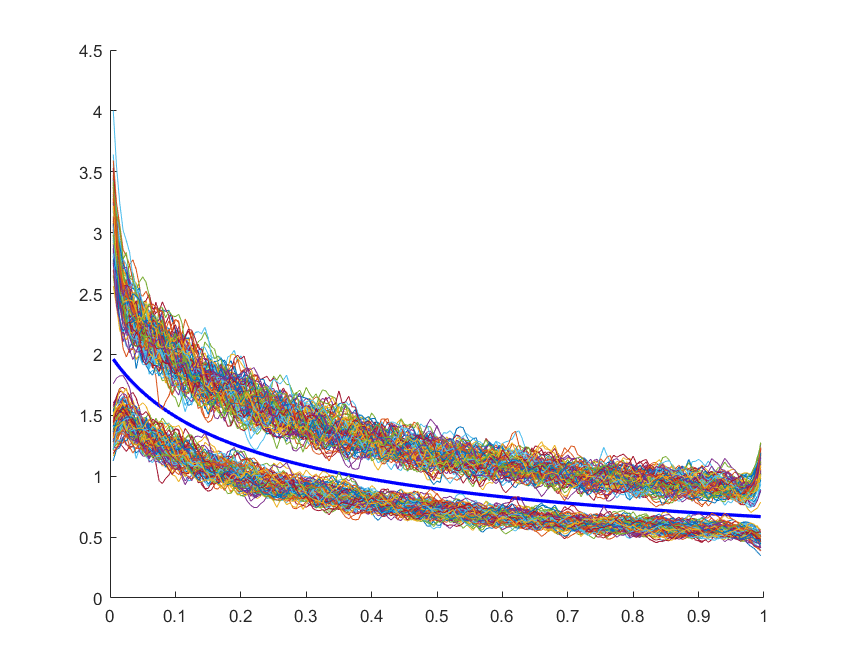
I consider the following distributions of the data, all supported on the interval : (i) uniform[0,1] distribution (ii) the distribution truncated to (iii) the linear distribution with the PDF , . I set the nominal confidence level to be and the sample size . The critical values are obtained by simulating and calculating the quantiles of its supremum on the grid , with the number of simulations set to (simulation results for the critical values based on are very similar, so I do not report them here). I use the kernel corresponding to the standard normal distribution truncated to and the nearly-optimal bandwidth , where I set since the scale of the bandwidth is , see Section 3.
In Figure 1, included for illustration, I plot 100 independent realizations of the confidence bands for the linear distribution, along with the true quantile density (in blue). Table 1 contains simulated coverage values for the two-sided confidence bands. The coverage is almost invariant to the distribution of the data, but the size distortion tends to be smaller for higher nominal confidence levels.
| Confidence level | ||||
| Uniform distribution | ||||
| 0.891 | 0.936 | 0.962 | 0.986 | |
| 0.881 | 0.943 | 0.966 | 0.990 | |
| 0.898 | 0.947 | 0.970 | 0.993 | |
| 0.907 | 0.949 | 0.976 | 0.996 | |
| Linear distribution | ||||
| 0.891 | 0.929 | 0.956 | 0.987 | |
| 0.878 | 0.936 | 0.961 | 0.989 | |
| 0.890 | 0.944 | 0.970 | 0.991 | |
| 0.914 | 0.949 | 0.976 | 0.996 | |
| Truncated normal distribution | ||||
| 0.898 | 0.942 | 0.964 | 0.988 | |
| 0.887 | 0.944 | 0.967 | 0.992 | |
| 0.905 | 0.950 | 0.972 | 0.993 | |
| 0.911 | 0.952 | 0.978 | 0.997 | |
6 Conclusion
To the best of my knowledge, no boundary bias correction or uniform inference procedures have been developed for the quantile density (sparsity) function. In this paper, I develop such procedures, establish their validity and show in a set of Monte Carlo simulations that they perform reasonably well in finite samples. I hope that, even when the quantile density itself is not the main inference target, these results may be employed for improving the quality of inference for other statistical objects, including the quantile function.
References
- Andreyanov and Franguridi (2022) Andreyanov, P. and G. Franguridi (2022): “Nonparametric inference on counterfactuals in first-price auctions,” Available at https://arxiv.org/pdf/2106.13856.pdf.
- Bahadur (1966) Bahadur, R. R. (1966): “A note on quantiles in large samples,” The Annals of Mathematical Statistics, 37, 577–580.
- Bloch and Gastwirth (1968) Bloch, D. A. and J. L. Gastwirth (1968): “On a simple estimate of the reciprocal of the density function,” The Annals of Mathematical Statistics, 39, 1083–1085.
- Chernozhukov et al. (2014a) Chernozhukov, V., D. Chetverikov, and K. Kato (2014a): “Anti-concentration and honest, adaptive confidence bands,” The Annals of Statistics, 42, 1787–1818.
- Chernozhukov et al. (2014b) ——— (2014b): “Gaussian approximation of suprema of empirical processes,” The Annals of Statistics, 42, 1564–1597.
- Csörgő et al. (1991) Csörgő, M., L. Horváth, and P. Deheuvels (1991): “Estimating the quantile-density function,” in Nonparametric Functional Estimation and Related Topics, Springer, 213–223.
- Csörgő and Révész (1981a) Csörgő, M. and P. Révész (1981a): Strong approximations in probability and statistics, Academic Press.
- Csörgő and Révész (1981b) ——— (1981b): Two approaches to constructing simultaneous confidence bounds for quantiles, 176, Carleton University. Department of Mathematics and Statistics.
- Falk (1986) Falk, M. (1986): “On the estimation of the quantile density function,” Statistics & Probability Letters, 4, 69–73.
- Giné and Guillou (2002) Giné, E. and A. Guillou (2002): “Rates of strong uniform consistency for multivariate kernel density estimators,” in Annales de l’Institut Henri Poincare (B) Probability and Statistics, Elsevier, vol. 38, 907–921.
- Jones (1992) Jones, M. C. (1992): “Estimating densities, quantiles, quantile densities and density quantiles,” Annals of the Institute of Statistical Mathematics, 44, 721–727.
- Kiefer (1967) Kiefer, J. (1967): “On Bahadur’s representation of sample quantiles,” The Annals of Mathematical Statistics, 38, 1323–1342.
- Kim and Pollard (1990) Kim, J. and D. Pollard (1990): “Cube root asymptotics,” The Annals of Statistics, 191–219.
- Koenker (2005) Koenker, R. (2005): Quantile Regression, Econometric Society Monographs, Cambridge University Press.
- Nolan and Pollard (1987) Nolan, D. and D. Pollard (1987): “U-processes: rates of convergence,” The Annals of Statistics, 780–799.
- Siddiqui (1960) Siddiqui, M. M. (1960): “Distribution of quantiles in samples from a bivariate population,” Journal of Research of the National Bureau of Standards, 64, 145–150.
- Stroock (1998) Stroock, D. W. (1998): A concise introduction to the theory of integration, Springer Science & Business Media.
- Tukey (1965) Tukey, J. W. (1965): “Which part of the sample contains the information?” Proceedings of the National Academy of Sciences, 53, 127–134.
- Welsh (1988) Welsh, A. (1988): “Asymptotically efficient estimation of the sparsity function at a point,” Statistics & Probability Letters, 6, 427–432.
Appendix
Appendix A Proof of Theorem 1 and 1
First, note that
| (28) | ||||
| (29) |
where uniformly in since is continuously differentiable on .
Therefore,
| (30) |
where
| (31) | ||||
| (32) |
The result now follows from the asymptotically linear expansion of the process ,
| (33) |
This expansion is implied by the proof of Andreyanov and Franguridi (2022, Theorem 1). I reproduce this proof here for completeness.
A.1 Proof of the representation (33)
First, we need the following two lemmas concerning expressions that appear further in the proof.
Proof.
Denote and note that is a function of bounded variation a.s. Using integration by parts for the Riemann-Stieltjes integral (see e.g. Stroock, 1998, Theorem 1.2.7), we have
| (35) |
To complete the proof, note that , , and . ∎
Proof.
Using integration by parts for the Riemann-Stieltjes integral (see e.g. Stroock, 1998, Theorem 1.2.7), we have
| (37) | ||||
| (38) |
where we used the fact that a.s. and a.s. We further write
| (39) | ||||
| (40) | ||||
| (41) | ||||
| (42) |
where in the second equality we used the change of variables . ∎
We now proceed with the proof of representation (33).
Recall the classical Bahadur-Kiefer expansion (Bahadur, 1966; Kiefer, 1967),
| (43) | ||||
| (44) |
and . Combine this expansion with Lemma 1 to obtain
| (45) | ||||
| (46) | ||||
| (47) |
First term in (47).
Since is bounded away from zero, for some constant , and hence . The first term in (47) can then be rewritten as
| (48) |
where
| (49) | ||||
| (50) |
the last equality using Lemma 2. The process has the strong uniform convergence rate (see, e.g., Giné and Guillou, 2002), and hence
| (51) |
Applying Lemma 2 to the first term in (48) allows us to rewrite
| (52) |
Second term in (47).
This term can be upper bounded as follows,
| (53) | |||
| (54) |
where we used the properties of total variation in the first inequality and in the second equality.
Note that we disregarded the term , since it has the uniform order , which is smaller than . Dividing by , which is bounded away from zero for due to Assumption 1, finishes the proof. ∎
A.2 Proof of 1
Let us check that the conditions of Giné and Guillou (2002, Proposition 3.1) hold. Indeed, Assumption 2 implies their condition , while Assumption 3 implies their conditions (2.11) and . By Giné and Guillou (2002, Remark 3.5), their condition can be replaced by the conditions satisfied by the uniform distribution. To complete the proof, divide the expansion in Theorem 1 by and note that the first term converges to by Giné and Guillou (2002, Proposition 3.1), while the remainder converges to zero a.s. due to Assumption 3. ∎
Appendix B Proof of Theorem 2
A key ingredient of the proof is to note that Lemmas 2.3 and 2.4 of Chernozhukov et al. (2014b) continue to hold even if their random variable does not have the form for the standard empirical process , but instead is a generic random variable admitting a strong sup-Gaussian approximation with a sufficiently small remainder.
For completeness, we provide the aforementioned trivial extensions of the two lemmas here, taken directly from Andreyanov and Franguridi (2022).
Let be a random variable with distribution taking values in a measurable space . Let be a class of real-valued functions on . We say that a function is an envelope of if is measurable and for all and .
We impose the following assumptions (A1)-(A3) of Chernozhukov et al. (2014b).
-
(A1)
The class is pointwise measurable, i.e. it contains a coutable subset such that for every there exists a sequence with for every .
-
(A2)
For some , an envelope of satisfies .
-
(A3)
The class is -pre-Gaussian, i.e. there exists a tight Gaussian random variable in with mean zero and covariance function
(56)
Lemma 3 (A trivial extension of Lemma 2.3 of Chernozhukov et al. (2014b)).
Suppose that Assumptions (A1)-(A3) are satisfied and that there exist constants , such that for all . Moreover, suppose there exist constants and a random variable such that . Then
| (57) |
where is a constant depending only on and .
Proof.
For every , we have
| (58) | ||||
| (59) | ||||
| (60) |
where Lemma A.1 of Chernozhukov et al. (2014b) (an anti-concentration inequality for ) is used to deduce the last inequality. A similar argument leads to the reverse inequality, which completes the proof. ∎
Lemma 4 (A trivial extension of Lemma 2.4 of Chernozhukov et al. (2014b)).
Suppose that there exists a sequence of -centered classes of measurable functions satisfying assumptions (A1)-(A3) with for each , where in the assumption (A3) the constants and do not depend on . Denote by the Brownian bridge on , i.e. a tight Gaussian random variable in with mean zero and covariance function
| (61) |
Moreover, suppose that there exists a sequence of random variables and a sequence of constants such that and . Then
| (62) |
Proof.
Take sufficiently slowly such that . Then since , by Lemma 3, we have
| (63) |
This completes the proof. ∎
I now go back to the proof of Theorem 2. Chernozhukov et al. (2014b, Proposition 3.1) establish a sup-Gaussian approximation of ; namely, there exists a tight centered Gaussian random variable in with the covariance function
| (64) |
where , such that, for , we have the approximation
| (65) |
Lemma 4 and Chernozhukov et al. (2014b, Remark 3.2) then imply
| (66) |
On the other hand, from Theorem 1 it follows that
| (67) |
where we define . Substituting (65) into (67) yields
| (68) |
Assumption 4 implies that and . Therefore,
| (69) |
It now follows from Chernozhukov et al. (2014b, Remark 3.2) that
| (70) |
Applying the triangle inequality to equations (66) and (70) yields
| (71) |
On the other hand, considering the sample , we have
| (72) |
A similar argument yields
| (73) |
which completes the proof. ∎