Bifurcation analysis of two-dimensional Rayleigh–Bénard convection using deflation
Abstract
We perform a bifurcation analysis of the steady states of Rayleigh–Bénard convection with no-slip boundary conditions in two dimensions using a numerical method called deflated continuation. By combining this method with an initialisation strategy based on the eigenmodes of the conducting state, we are able to discover multiple solutions to this non-linear problem, including disconnected branches of the bifurcation diagram, without the need for any prior knowledge of the solutions. One of the disconnected branches we find contains an S-shaped curve with hysteresis, which is the origin of a flow pattern that may be related to the dynamics of flow reversals in the turbulent regime. Linear stability analysis is also performed to analyse the steady and unsteady regimes of the solutions in the parameter space and to characterise the type of instabilities.
I Introduction
This paper considers the bifurcations of the two-dimensional Rayleigh–Bénard convection, which supports a profusion of states. There have been numerous investigations trying to visualise solutions and characterise the steady states of Rayleigh–Bénard convection, as well as computing its bifurcation diagrams with respect to , the Rayleigh number, in various settings and for different geometries [1, 2]. Ouertatani et al. [3] performed numerical simulations of Rayleigh–Bénard convection in a square cavity using the finite volume method and computed fluid flow profiles and temperature patterns at . Numerical studies have been conducted to understand the existence of bifurcating solutions to this problem in a two-dimensional domain with periodic boundary conditions in the horizontal direction [4, 5]. Mishra et al. [6] analysed the effect of low Prandtl number on the bifurcation structures, while Peterson [7] used arclength continuation [8] to study the evolution of cell solutions with respect to the aspect ratio of the domain. Bifurcation structures of Rayleigh–Bénard convection have been extensively studied in cylindrical geometry by Ma et al. [9] as well as by Borońska and Tuckerman [10, 11]. In particular, references [10, 11] adapted a time-dependent code to perform branch continuation and then analysed the linear stability of the computed solutions using Arnoldi iterations [12]. Finally, Puigjaner et al. [13, 14] computed bifurcation diagrams for Rayleigh–Bénard convection in a cubical cavity over different intervals of .
A common way to reconstruct bifurcation diagrams is to use arclength continuation and branch switching techniques [15, 8, 16] to continue known solutions in a given parameter. These solutions can be computed by applying Newton’s method to suitably chosen initial guesses or by using time-evolution algorithms. A standard numerical technique in fluid dynamics for finding initial states for the continuation algorithm is to perform time-dependent simulation of initial solutions until a steady state is reached [17, 18, 19]. These numerical techniques have been widely used and are extremely successful at computing bifurcation diagrams of nonlinear PDEs.
In this paper, we employ a recently developed algorithm called deflation for computing multiple solutions to nonlinear partial differential equations [20, 21]. This method has been successfully applied to compute bifurcations to a wide range of physical problems such as the deformation of a hyperelastic beam [21], Carrier’s problem [22], cholesteric liquid crystals [23], and the nonlinear Schrödinger equation in two and three dimensions [24, 25, 26]. We emphasise that deflation offers some advantages that could be combined with the standard bifurcation analysis tools. The main strength of deflation is that it detects of disconnected branches, in addition to those connected to known branches. An additional advantage is that it does not require the solution of augmented problems to find new solutions. Using perturbed solutions to the linearised equations as initial conditions, we are able to discover numerous steady states of Rayleigh–Bénard convection. These solutions can be obtained without prior knowledge and regardless of the stability of the solutions.
While much progress in fluid dynamics has been made on the study of hydrodynamic instabilities, instabilities that occur when a control parameter is varied within the turbulent regime remain poorly understood [27]. The difficulty in studying such transitions arises from the underlying turbulent fluctuations which make analytical approaches cumbersome. These types of transitions resemble more closely phase transitions in statistical mechanics because the instability occurs on a fluctuating background [28]. In Rayleigh–Bénard convection, such transitions have been observed in the form of reversals of the large scale circulation in an enclosed rectangular geometry, both in experiments and numerical simulations [29, 30, 31]. Although we do not study the turbulent case, we investigate the bifurcations of Rayleigh–Bénard convection in an enclosed rectangular geometry to attempt to understand the genesis of the flow patterns that play the central role in flow reversals in the turbulent regime.
The paper is organised as follows. We first discuss the problem set-up and the choice of parameters in Section II. Then, in Section III, we briefly review deflation and present the methods used to improve its initialisation procedure and compute the linear stability of the solutions. Next, we analyse the different branches discovered by deflation and their stability in Section IV. Finally, in Section V, we recapitulate the main conclusions of this study and propose potential extensions for future work.
II Problem set-up
We consider Rayleigh–Bénard convection [32, 33, 34] in a confined fluid heated from below and maintained at a constant temperature difference across a two dimensional square cell of height . For simplicity, we employ the Oberbeck–Boussinesq approximation [35, 36, 37] in which the kinematic viscosity and the thermal diffusivity do not depend on temperature while the fluid density is assumed to be constant except in the buoyancy term of the momentum equation. In this case, we assume the density to depend linearly on the temperature, , where is the thermal expansion coefficient. Then, the governing equations of the problem are
| (1a) | ||||
| (1b) | ||||
| (1c) | ||||
where is the velocity field, is the temperature field, is the pressure, and is the buoyancy direction. The above equations have been nondimensionalized using , and as the relevant scales for length, time and temperature, respectively. The two dimensionless parameters of the problem are the Rayleigh and Prandtl numbers
| (2) |
where is the gravitational acceleration. The Rayleigh number represents the ratio of the acceleration related to buoyancy to the stabilizing effects of and . The bifurcation parameter in the problem we study is by fixing . The cell is assumed to have rigid walls, with thermally conducting horizontal walls and thermally insulating side walls, i.e.
| (3a) | ||||
| (3b) | ||||
| (3c) | ||||
| (3d) | ||||
The trivial steady state is motionless with a negative thermal gradient through the layer,
| (4) |
and is called the conducting state. This is because the fluid acts as a conducting material. The cooler fluid near the top of the layer is denser than the warmer fluid underneath it. The symmetries of the problem are: a) the mirror symmetry with respect to the axis
| (5) |
which leaves the velocity and temperature field invariant, and b) the Boussinesq symmetry
| (6) |
which leaves the velocity field invariant but transforms the temperature field into its opposite. These symmetries (and the combination of both) dictate the bifurcations that the system can undergo.
III Numerical methods
III.1 Computation of multiple solutions with deflation
Steady states of Rayleigh–Bénard convection are computed using a recent numerical technique called deflation [20]. This algorithm is based on Newton’s method and can compute multiple solutions to a nonlinear system of equations , where is the solution and is a bifurcation parameter. First, fix and assume a solution to has been previously discovered by Newton’s method. One can then construct a deflated problem
| (7) |
such that does not converge to zero as . The term is called a deflation operator and ensures that Newton’s method applied again to will not converge to a previously computed solution. By adding one to the expression of the deflation operator, we impose that the new problem behaves similarly to away from the root . This process can be repeated to obtain a set of solutions to a nonlinear problem at the bifurcation parameter . Deflated continuation is the combination of this idea with continuation. The previously discovered solutions are continued to a new bifurcation parameter : each is used as an initial guess for the deflation procedure in order to construct a new set of solutions at .
We apply this algorithm repeatedly to discover multiple solutions to the steady state Rayleigh–Bénard problem:
| (8) |
where and is the bifurcation parameter. This equation is discretised with Taylor–Hood finite elements for the velocity and pressure (piecewise biquadratic and piecewise bilinear respectively), together with piecewise bilinear polynomials for the temperature, using the Firedrake finite element library [38]. The unit square domain is represented by a mesh with square cells to preserve the symmetries of the problem and avoid spurious symmetry breaking solutions. A coarse discretization is needed due to the complexity of the problem and number of distinct solutions discovered. However, we did not observe significant differences in selected experiments where we refined the mesh.
Deflated continuation requires two different computational tasks. The first is the continuation of a previously discovered branch by the continuation step, which usually results in the convergence of the Newton solver in an average of three iterations. The convergence criterion is defined to be when the Euclidean -norm of the discretised PDE residual is below . The second task is the deflation step to discover new branches. Most of the time, the solver does not converge, which means that it does not discover any new branch within the maximum number of Newton iterations allowed, which is set to one hundred. Typically, when the deflation step is successful, it requires around iterations to find a new solution. Since the deflation step is employed for each of the steady states in the different branches, this yields at least hundreds of thousands of Newton iterations in total, and a few weeks of calculation on a desktop with 32 cores. The linear systems resulting from Newton’s method are solved using the sparse direct solver MUMPS [39].
A crucial question in the deflation technique is the choice of the deflation operator because it can affect the convergence of Newton’s method. We use the following operator,
| (9) |
where denotes the -norm. Note that the deflation operator does not depend on the pressure because we wish to deflate all the solutions of the form , where , to avoid discovering solutions trivially related to known ones.
We perform bifurcation analysis of Rayleigh–Bénard convection and compute solutions to the nonlinear system of Eq. 8 for using deflated continuation for . Here, denotes the continuation step size in the bifurcation parameter, which is chosen as . In a previous work on the computation of solutions to the 3D nonlinear Schrödinger equation [26], we found that having good initial guesses (e.g. solutions of the linearised problem) for the initial deflation steps facilitates the convergence of Newton’s method and leads to more complex and interesting states. However, contrary to [26] we do not have the analytic expressions of the linear solutions to the Rayleigh–Bénard convection due to the no-slip boundary conditions. Therefore, we numerically solve an eigenvalue problem (see Section III.2) to obtain the first ten unstable eigenmodes linearised around the conducting steady state Eq. 4 (see Fig. 2). Then, the sums of the conducting state with the respective normalized perturbations: are used as initial guesses for deflated continuation.
III.2 Linear stability analysis
The stability analysis of a given steady state is performed by considering the perturbation ansatz
| (10a) | ||||
| (10b) | ||||
where the velocity perturbation and the temperature perturbation have an eigenvalue , whose real part is the growth rate and imaginary part is the frequency of the corresponding eigenvector. When at least one of the eigenvalues has a positive real part , we can have two types of instabilities: to a real eigenmode, occurring when the imaginary part of the eigenvalue , and to a complex eigenmode, occurring when . If all the eigenvalues have negative real parts, then the steady state is stable. Inserting Eq. 10 into Eq. 1 and considering the linearised system of equations, we obtain the following generalised eigenvalue problem at leading order
| (11) |
where is the relevant identity operator and is the linear operator defined by
The eigenvalue problem described in Eq. 11 is solved with a Krylov–Schur method [40] using the SLEPc library [41].
To obtain the critical value of the Rayleigh number at which the conducting state Eq. 4 becomes unstable, we modify the eigenvalue problem in Eq. 11. Inserting Eq. 4 into Eq. 11 we obtain the following generalized eigenvalue problem
| (12) |
A steady state becomes unstable when and this corresponds to the critical Rayleigh number which is the smallest satisfying Eq. 12 for . So, to obtain the critical value of the Rayleigh number for different base states we have reformulated the problem to a generalised eigenvalue problem for as follows
| (13) |
In the following sections this linear analysis will be used to study the stability of the conducting state Eq. 4 and of the nonlinear steady states that we obtain from deflated continuation.
IV Results
IV.1 Primary instabilities
In this section, we analyse the stability of the conducting steady state defined by Eq. 4. We found that the first instability of this state arises at . It is well known [42] that the critical Rayleigh number is approximately equal to for a domain with periodic side boundaries and no-slip top and bottom boundaries. This difference in the value of is due to the effect of the side walls on the instability. This effect should decrease when the length of the domain, , becomes large such that the behaviour predicted for an unbounded domain is recovered. To demonstrate this, we systematically increase the aspect ratio
| (14) |
Figure 1 (left) clearly shows that for the converges to .
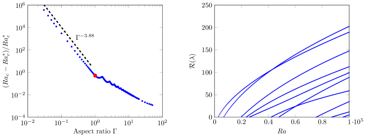
In addition, for aspect ratios we observe . The critical Rayleigh number for Rayleigh–Bénard convection with stress-free boundary conditions is [43], where is the horizontal wavenumber. For the critical Rayleigh number scales like using Eq. 14. This scaling relation is very close to the observed one, which implies that the exponent is not affected much by the no-slip boundary conditions. The exponent we find is in agreement with [44].
| 1 | 2 | 3 | 4 | 5 | 6 | 7 | 8 | 9 | 10 | |
| 2586 | 6746 | 19655 | 23346 | 25780 | 41772 | 47431 | 74878 | 86313 | 94543 | |
| (1,1) | (2,1) | (3,1) | (2,2) | (1,2) | (3,2) | (4,1) | (4,2) | (2,3) | (3,3) |
The case on which we focus for the rest of the paper is the square cell (), which is denoted with a red dot in Fig. 1 (left). We first study the linear stability of the conducting state Eq. 4. In the range we observe 10 supercritical stationary bifurcations that arise from the conducting state. Figure 1 (right) shows the growth rates of the unstable eigenmodes as a function of . These bifurcations occur when . The critical values of the Rayleigh number at the onsets are listed in Table 1. Fig. 1 (right) demonstrates that the growth rates of the eigenmodes vary with Rayleigh number such that the curves can cross. The eigenmode which bifurcated from the conducting state at ends up being the most unstable as .
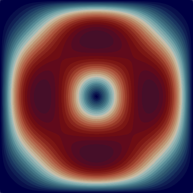
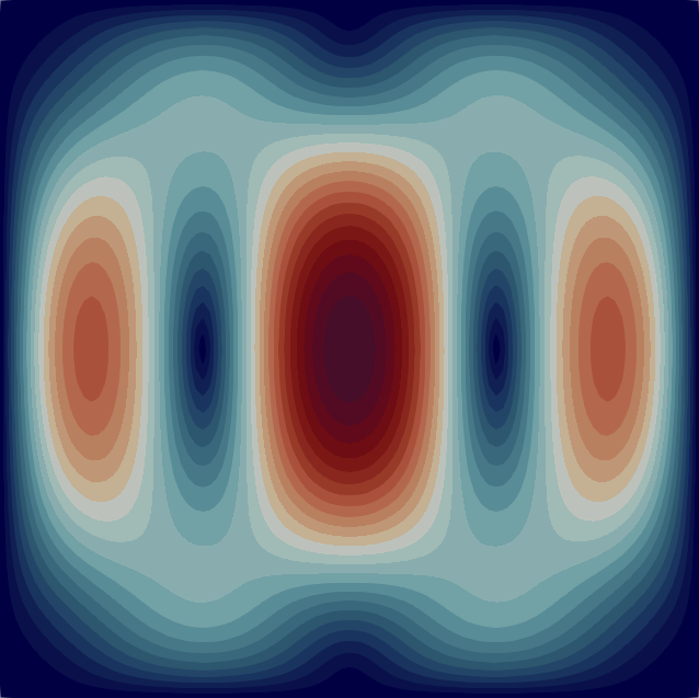
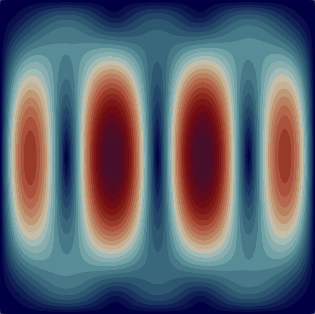
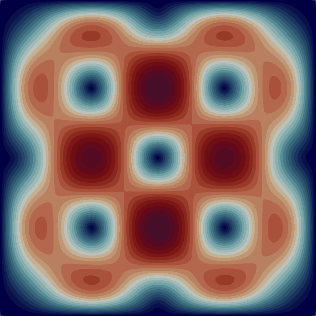
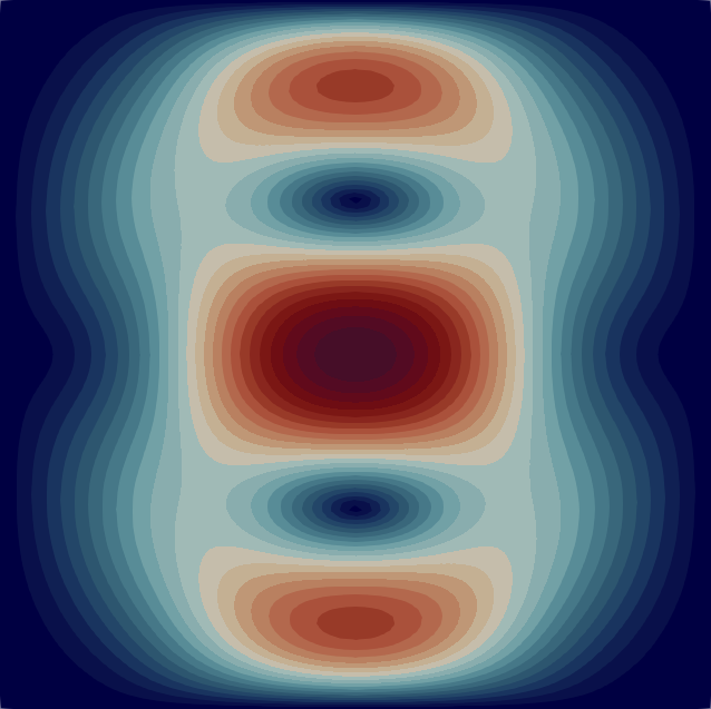
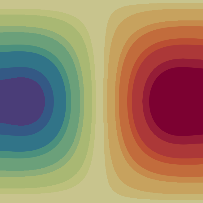
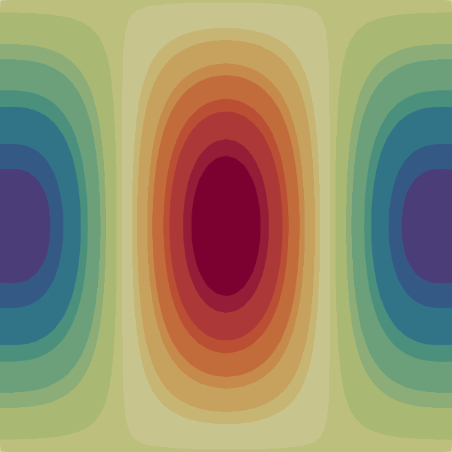
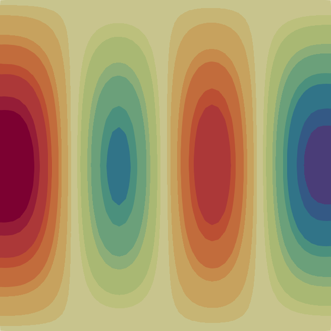
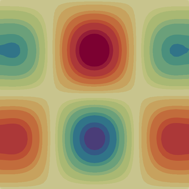
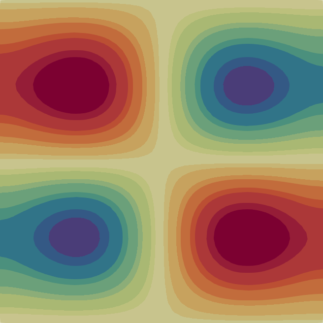
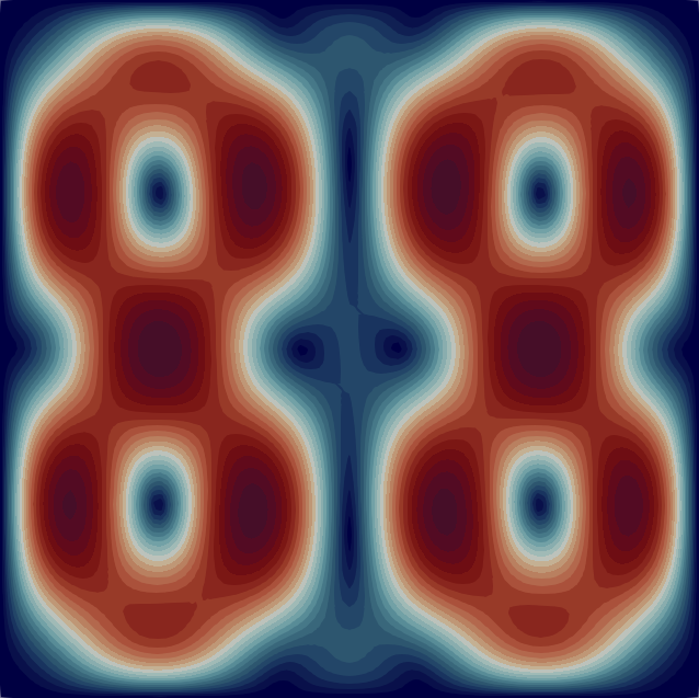
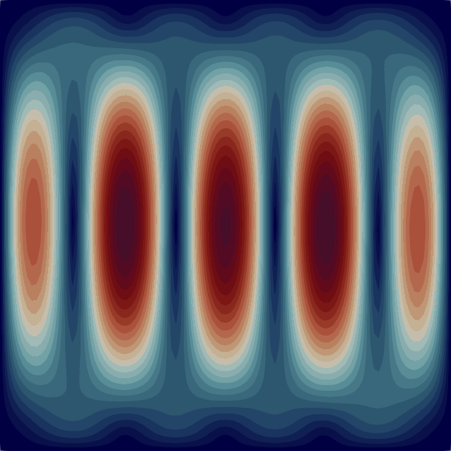
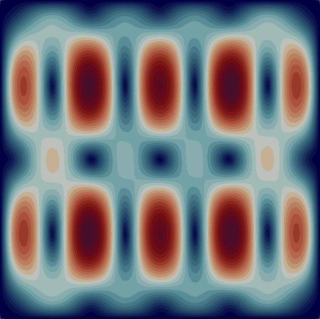
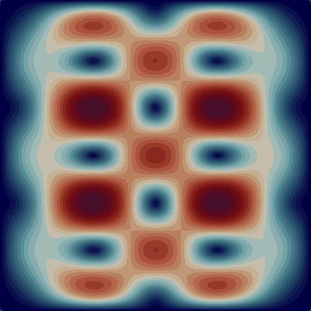
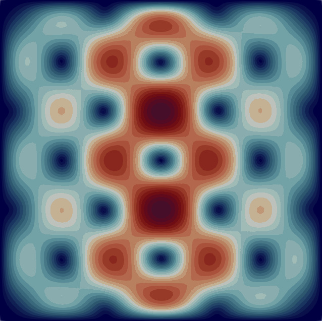
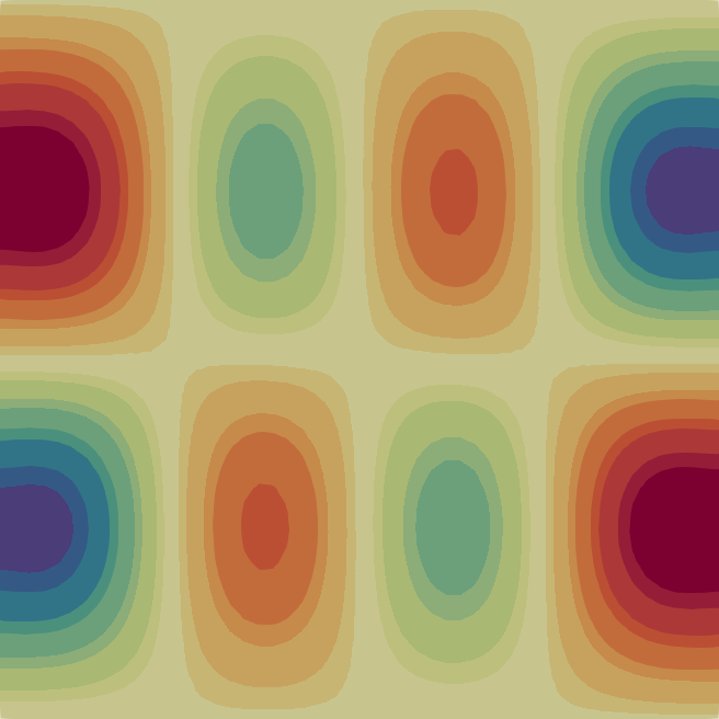
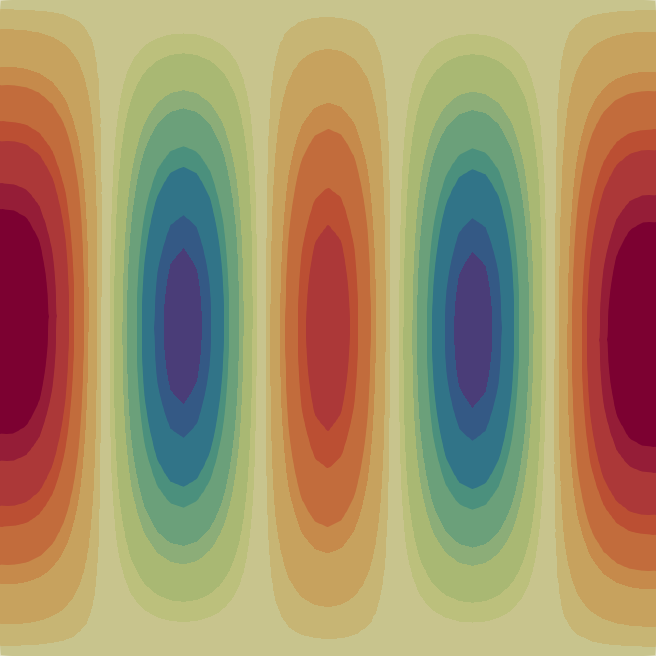
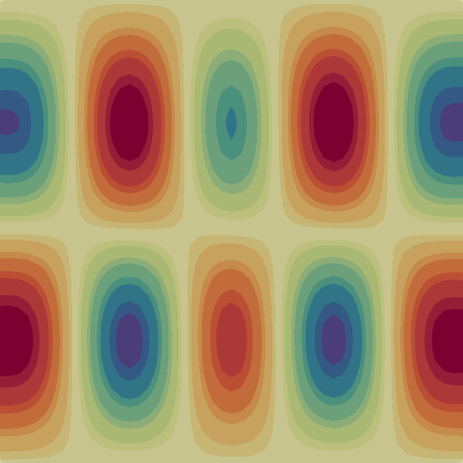
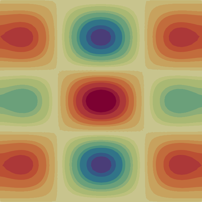
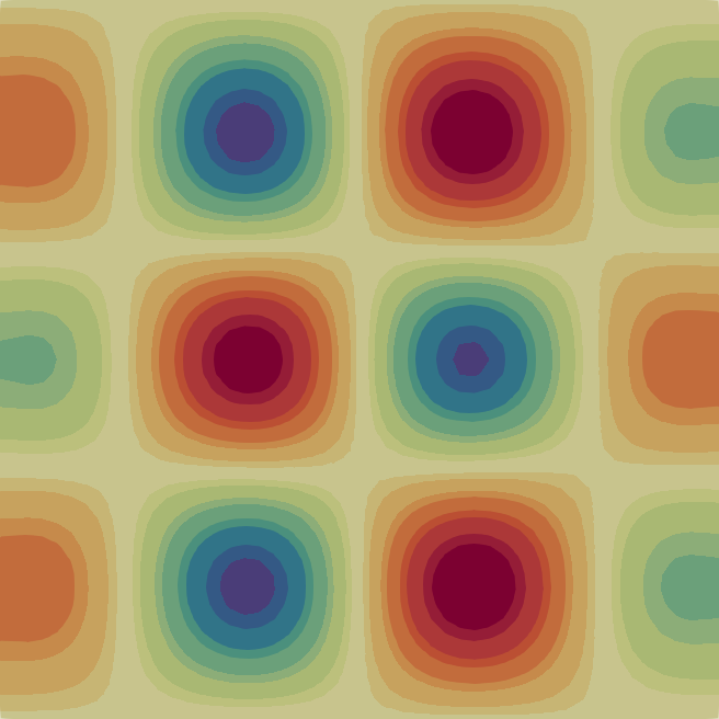
The velocity magnitude and temperature fields of the eigenmodes from these primary bifurcations of the flow are shown in Fig. 2 with the corresponding critical Rayleigh numbers indicated on the top of each flow pattern. In Table 1 we characterise the flow patterns by the number of rolls , where and are the number of rolls in the temperature field in the horizontal and vertical direction, respectively. Note that due to the aspect ratio of the domain the flow pattern of the first bifurcation at is just a single convection roll (see Fig. 2) according to the classical result [33]. In the following sections, we first analyse the branches of solutions that are created from some of these primary bifurcations before moving to disconnected branches.
IV.2 Bifurcation diagrams
The combination of deflation and the initialisation strategy presented in Section III.1 identified branches for the two-dimensional steady-state Rayleigh–Bénard convection at , leading to branches when reflections are included. Here, we analyse the evolution and the linear stability of some of the branches arising from the first four excited states (see Fig. 2) as well as two disconnected branches. Moreover, we discard the mirror symmetric solutions with respect to the and axes (see symmetries in Section II). Our diagnostics for the bifurcation diagrams, representing the evolution of the steady states as a function of , are the kinetic energy , the potential energy , and the Nusselt number , which are defined as
| (15) |
The Nusselt number characterises the efficiency of convective heat transfer and is given by the ratio of the total heat transfer (i.e. both advective and diffusive) to the conductive heat transfer , where is the heat flux and stands for the area average. A Nusselt number of one represents heat transfer by pure conduction. Here, the Nusselt number is essentially defined as the dissipation rate of the temperature variance (see second equality). This is obtained by integrating the equation for potential energy over the entire area [45].
The bifurcation diagrams are presented in Fig. 3, where the numbers denote the different branches of steady solutions, indicating the values of kinetic energy, potential energy and Nusselt number that correspond to each branch on each diagram.
The first steady solutions that we obtain from deflated continuation as is varied are four branches that arise from the first four bifurcations of the conducting steady state: branch (1) at , branch (2) at , branch (3) at and branch (4) at . Moreover a secondary branch (10) bifurcates at from branch (2), which originates from the second instability of the conducting state. A similar behaviour is observed for the fourth instability, where branch (6) bifurcates at from branch (4). We also focus on two disconnected branches (11) and (8) obtained directly by deflated continuation. In Fig. 3(a), branch (11) is close to branch (12). However, note that the bifurcation diagram using the potential energy (see Fig. 3(b)) shows that branch (11) does not bifurcate from branch (12). On the other hand, branch (8) bifurcates from branch (11) at (see Fig. 3). It is interesting to point out that in the range branch (1) has the highest kinetic energy while branch (6) has the highest potential energy (see Fig. 3(a) and 3(b)). The steady states that are most effective in convecting heat transfer for are in branch (1) from the first instability of the conducting state while for are in the branch (2), and in branch (11) for (see Fig. 3(c)).
IV.3 Bifurcations from the conducting steady state
In this section we analyse the states that emanate from the conducting steady state and their evolution as a function of the bifurcation parameter . Our analysis involves the detailed evolution of the velocity magnitude and the temperature on the branches of the bifurcation diagrams using the kinetic and potential energy, respectively. In addition, we present the largest growth rates and corresponding frequencies from the linear stability analysis we have performed on the steady states.
Figure 4 shows results of the aforementioned analysis for branch (1), which arises at from the first eigenmode (see Fig. 2). This bifurcation breaks the -reflection symmetry but the branch has the Boussinesq symmetry. As increases, the magnitude of the velocity field evolves from a circular to a bent convection roll at (see Fig. 4(a)). On the other hand, the -shaped interface of the temperature field is sheared (see Fig. 4(b)), enhancing the heat transfer in the convection cell (see also branch (1) in Fig. 3(c)). Fig. 4(c) demonstrates that the solutions on this branch remain stable () with an almost constant growth rate over the whole range of Rayleigh numbers we consider. The frequency corresponding to the largest growth rate is zero from the stationary bifurcation at to the (see Fig. 4(d)), while the next eigenvalue has a negative real part and a large imaginary part.
The second eigenmode introduced in Fig. 2 gives birth to branch (2) at , which is depicted in Fig. 5(a)-(b). The bifurcation is transcritical and preserves the symmetries of the eigenmode in the velocity and temperature profiles. Then, the largest growth rate in Fig. 5(c) indicates that the solutions on this branch are stable over the interval and unstable outside. A bifurcation occurs at when , which is analysed later and illustrated in Fig. 6. The bifurcation from branch (2) to branch (10) is accompanied by a loss of Boussinesq symmetry. Another bifurcation is observed at and has been obtained by deflated continuation.
Figure 6(a) demonstrates that the two symmetries of the second eigenmode (see Section II) are rapidly broken as increases after the bifurcation from branch (2) to the secondary branch (10). This symmetry breaking leads to a primary large scale circulation spanning the domain and a secondary vortex with smaller amplitude in one of the corners depending on which symmetric solution one is referring to. As , the difference in the flow pattern of the velocity magnitude between branch (1) and (10) is the secondary vortex in the corner of the convection cell. The symmetry breaking is also obvious in the temperature field (see Fig. 6(b)) with the potential energy of the flow increasing and then decreasing slightly in contrast to the increase of the kinetic energy and the convective heat transfer (see also Fig. 3(c)). The largest growth rate shows that the states are unstable to a real eigenmode (see Fig. 6(d)). The subsequent growth rates shown in Fig. 6(c) are negative and almost constant in this range of Rayleigh numbers.
Branch (3) originates from the eigenmode of the conducting state at , which is depicted in Fig. 7. This branch preserves the centro-symmetry of the 3rd eigenmode and has a turning point located at . Interestingly, the lower part of the branch, coloured in red in Fig. 7(a,b) bifurcates from branch (5) around . The latter branch emanates from the fourth eigenmode and is illustrated later in Fig. 10. The largest growth rates of the upper and lower parts of branch (3) are displayed in Fig. 7(c,d), together with their associated frequencies. We find that the steady states in the branch are unstable with a zero frequency throughout the range of Rayleigh numbers for which the branch exists. Moreover, we observe that the eigenmode coloured in purple in Fig. 7(c) traverses zero at , indicating the presence of a secondary bifurcation, which we will analyse in the following paragraph. We point out that this branch has not been originally discovered by deflated continuation (our method does not guarantee to find all the steady states of a problem) but obtained by continuing the third linear state with finer steps in the Rayleigh number. This illustrates that deflated continuation may be complemented by standard bifurcation analysis techniques, such as arclength continuation and branch-switching algorithms.
We now focus on branch (12), which bifurcates from branch (3) at , and display the evolution of the steady states in the branch in Fig. 8 along with its stability analysis. This branch breaks the centro-symmetry of branch (3) and the pattern of the velocity magnitude becomes more complex as increases. This complex pattern is one reason for the meandering of the potential energy in this range of Rayleigh numbers and enhances the convective heat transfer (see Fig. 3(c)) by mixing the temperature field. Fig. 8(c) shows that the steady states of branch (12) are unstable to two eigenmodes until , where they coalesce. At this Rayleigh number, we see that the two most unstable eigenmodes coalesce into an unstable complex conjugate pair of eigenvalues (see Fig. 8(d)). All the subsequent eigenmodes are found to be stable with either or .
Fig. 10 shows bifurcation diagrams and the linear stability results of branch (4) which originates from the fourth eigenmode at through a transcritical bifurcation. The flow pattern of the velocity magnitude has a symmetric form of an array of four vortices, which is conserved over the whole range of the Rayleigh numbers we consider as Fig. 10(a) suggests. Similarly, the symmetric pattern of the temperature field remains unaffected in the regime (see Fig. 10(b)). We have verified numerically that the symmetries are conserved within this range of . Fig. 10(c) shows the four largest growth rates as a function of . At Rayleigh numbers close to we see that three of the eigenmodes are real and unstable, while the fourth one is real and stable. As increases, the two most unstable eigenmodes (coloured in red and green, respectively, in Fig. 10(c)) coalesce at into a complex unstable eigenmode whose growth rate and oscillation frequency increases as . Similarly, the other two real unstable modes coalesce at into a complex conjugate pair of eigenmodes which are unstable for . At and , we observe in Fig. 10(c) that the growth rate coloured in blue vanishes with a nonzero frequency, leading to Hopf bifurcations where periodic solutions to the time-dependent problem (1) arise.
We close our discussion on the branches arising from the conducting steady state with branch (5), presented in Fig. 10. This branch originates from the fourth eigenmode of the conducting state at through the same transcritical bifurcation as branch (4). The steady states in branch (5) conserve the Boussinesq and symmetries, with a velocity field consisting of four vortices, located symmetrically at each corner of the domain. The velocity fields of branches (4) and (5), illustrated in Fig. 11, are different, indicating that branch (5) is not a symmetric version of branch (4). The stability analysis reveals that the steady states in this branch are very sensitive to perturbations and unstable to a real eigenmode throughout the range of considered in this study. Moreover, the largest growth rate at is equal to , which is approximately three times larger than the largest growth rate of the steady state in branch (4) at the same Rayleigh number (see Fig. 10(c) and Fig. 10(c)). One of the eigenmodes vanishes at giving rise to branch (3), depicted in Fig. 7. Finally, the real part of the eigenvalue depicted in blue in Fig. 10(c-d) crosses zero at , which shows the existence of a Hopf bifurcation.
We now analyze the branches bifurcating from branches (4) and (5). The fourth largest growth rate of branch (4), coloured in blue in Fig. 10(c), crosses zero at , leading to the bifurcating branch (6) depicted in Fig. 13. We observe that the Boussinesq symmetry of branch (4) is broken by the bifurcation, while the symmetry with respect to the axis is preserved. Additionally, the linear stability analysis indicates that this branch is unstable with a zero frequency except in the interval , where the largest growth rate is associated with a positive frequency, as shown by the eigenvalues coloured in blue in Fig. 13(a) and (c). Moreover, the third largest growth rate (coloured in orange) crosses zero around , indicating the presence of a bifurcation which has not been discovered by deflation.
Finally, a branch, denoted by branch (7), bifurcates from branch (5) at . The steady states in this branch are illustrated in Fig. 13. We observe on the velocity magnitude and temperature field that the symmetry of branch (5) with respect to the axis is maintained while the Boussinesq symmetry is broken. Branches (6) and (7) might seem nearly symmetric but they arise at different Rayleigh numbers and have different eigenvalues. The linear stability analysis of branch (7) shows that the steady states are unstable to a real eigenmode, with a largest growth rate around throughout the range of considered in this study. In Fig. 13(c) and (d), we observe that the third eigenvalue (plotted in green) crosses zero at , resulting in a tertiary branch that breaks the remaining symmetry. The branch has been discovered by deflation but we chose to not report it in the study.
IV.4 Disconnected branches
We now focus on the disconnected branch (11) (see Fig. 3), which comprises an upper and a lower branch, depicted in blue and red in Fig. 14, respectively. At the upper (blue) branch the flow pattern of the velocity magnitude is a three vortex state with one large titled vortex spanning the domain and two smaller vortices located at the corners. As we notice that the state looks similar to the branches (1) and (10). The difference is that branch (10) involves only one smaller vortex at the corner of the domain and branch (1) has no vortices at the corners, while branch (11) has two smaller vortices located at the corners. At the branch takes the form of an S-shaped curve with hysteresis, similar to the cusp bifurcation [46].
As the saddle-node bifurcation is approached from below, the growth rate of the most unstable eigenmode decreases toward zero at the critical point (see Fig. 14(c)). Above the bifurcation point increases and seems to saturate as . The frequency corresponding to the growth rate is zero in the whole range of numbers suggesting that the steady state is unstable to a real eigenmode in this regime. The potential energy of the upper (blue) branch decreases with in contrast to the kinetic energy. As increases the flow pattern of the temperature becomes more efficient at transferring heat due to the large scale circulation in the flow (see Fig. 3(c)). The flow pattern of the velocity of the upper (blue) branch, shown for (see Fig. 14(a)), exhibits a large scale vortex and two smaller vortices at the corners of the domain. This is reminiscent of the flow patterns from studies on the dynamics of random-in-time flow reversals [47, 29, 30, 31]. These reversals in the flow direction of the large scale circulation at irregular time intervals have been observed in domains with free-slip or no-slip boundaries and in a narrow band of Rayleigh numbers in the range depending on the Prandtl number [29, 30, 31]. In this regime the system fluctuates in time between essentially the state we show for (see Fig. 14(a)) and its mirror symmetric state. These large changes in the dynamics of the flow are caused by bifurcations over a turbulent background [27]. Such bifurcations have been observed in many other types of flows [48, 49, 50, 51, 52] and understanding their dynamics is an open question of great interest.
At the lower (red) branch illustrated in Fig. 14(a) we observe the central vortex to be oriented more vertically, giving space to the smaller vortices at the corners to extend along the axis and almost reach the height of the domain. This flow pattern is an extension of the two-vortex pattern observed in branch (5) (see Fig. 6) and it has similar features to the three-vortex pattern found near the linear limit of branch (3) (see Fig. 7). The patterns of the kinetic and potential energy of this branch are almost invariant within the range . The flow pattern of the temperature clearly manages to effectively push the hot fluid toward the cold plate at the top and vice versa. This efficiency in convective heat transfer is clearly depicted in Fig. 3(c), where this part of branch (11) has the highest Nusselt number for . Analysing the stability of the lower (red) branch, we find that the steady solutions become increasingly more stable as the Rayleigh number increases, with at , leading to a Hopf bifurcation (see Fig. 14(e)). On the other hand, the frequency corresponding to the growth rate satisfies at the threshold of the disconnected branch and as increases the instability becomes progressively oscillatory (see Fig. 14(f)). The subsequent growth rates presented in Fig. 14(e) remain negative as increases suggesting that this part of branch (11) is another preferred steady state of the system particularly for .
Branch (8) illustrated in Fig. 15 bifurcates from the lower part of the disconnected branch (11) at (see also Fig. 3). In this case, the pattern of the velocity transitions into a main bent vortex with a vertically elongated vortex on its left and a smaller vortex at the bottom right corner (see Fig. 15(a)). From Fig. 3 we can see that even though the kinetic energy of branch (8) is equal to that of the upper part of branch (11) for , the potential energy is much smaller and apparently the smallest among the branches we have considered. The pattern of the temperature is essentially a hot plume that rises effectively all the way to the cold plate (see Fig. 15(b)). This flow pattern becomes increasingly more efficient at transferring heat across the domain as increases (see Fig. 3(c)). However, it is not as efficient in convecting heat as the pattern of branch (11) (see lower branch in 14(b)) because two hot plumes are obviously more effective than one. The steady state of branch (8) is unstable to a real eigenmode over the range except for a small range around where it becomes unstable to a complex eigenmode. This can be seen from Fig. 15(c) and 15(d), where the two largest growth rates (coloured in red and blue) swap with each other in this small range of Rayleigh numbers. Finally, the real part of the eigenvalue depicted in blue in Fig. 15(c-d) crosses zero at , giving birth to a Hopf bifurcation.
The second disconnected branch that we find in this range of Rayleigh numbers is branch (9) and arises at (see Fig. 16). From Fig. 16(a), we see that all the symmetries of the flow are broken in this branch and the flow pattern consists of a number of vortices with different orientations. These flow structures are not persistent over the range of parameters that we consider, and hence the heat is not transferred effectively across the domain (see also Fig. 3(c)). Here, Fig. 16 shows that the potential energy of branch (9) increases along with the kinetic energy unlike in most of the other branches we considered and from Fig. 3(b) we see that it is significant in comparison to many other branches. Moreover, from the linear stability analysis of the steady states we find that both the upper and lower parts of this disconnected branch are unstable to a real eigenmode, i.e. and , with large growth rates. This suggests that this branch is very unlikely to be observed in a laboratory experiment, and highlights the effectiveness of deflated continuation in identifying such unstable disconnected branches and steady states.
V Conclusions
In this work, we have computed and analysed the linear stability of steady states of the two-dimensional Rayleigh–Bénard convection in a square cell with rigid walls. The combination of deflated continuation and a suitable initialization procedure based on the linear stability of the motionless state is revealed to be a powerful numerical technique for finding multiple solutions including disconnected branches, which are not easily accessible by standard bifurcation techniques such as arclength continuation and time-evolution algorithms. A highlight is the success of deflation to discover these branches in an automated manner without any prior knowledge of the dynamics.
We classify the solutions based on the kinetic and potential energy as well as the Nusselt number. Our classification provides a clear view of the steady states of Rayleigh–Bénard convection up to a Rayleigh number of . We show that the steady states of branch (1) (which originates from the conducting state) dictate the dynamics of the flow for , while for the flow patterns of the disconnected branch (11) start to play a very important role as the steady states become stable. Solutions on branch (11) are reminiscent of the flow pattern that plays the fundamental role in the turbulent dynamics of flow reversals that have been reported in the literature for Rayleigh–Bénard convection at [29, 30, 31]. This disconnected branch exhibits an S-shaped curve with hysteresis which can be a challenge to discover with other bifurcation techniques.
There are several possible extensions to this work. An interesting but computationally challenging future study is to extend certain solutions of interest to higher values of and determine whether they give the required theoretical scalings in the limit of high Rayleigh number. A first attempt toward this direction has been done in Rayleigh–Bénard convection with periodic boundary conditions in the horizontal direction and no-slip in the vertical direction [53, 54]. Moreover, the extensions of branch (11) and its stability in the regime where reversals occur is also of great interest. Another extension of interest is to study how the states presented in this study change with respect to other parameters of the system such as the Prandtl number or the aspect ratio of the domain . As observed in the left panel of Fig. 1, the critical Rayleigh number converges to for large aspect ratio. Using alternative formulations of the Rayleigh–Bénard problem, with the aspect ratio playing the role of the bifurcation parameter, it is possible to analyse the evolution of the branches for large aspect ratio and connect them with the solutions of the periodic set-up, which has been studied well in the literature, both analytically [42] and numerically [4, 5]. This connection will be of great interest to theoreticians and hopefully will spark their interest to explore analytical solutions on more realistic convection set-ups with side walls.
A different future direction would be to perform bifurcation analysis on Rayleigh–Bénard convection in a three-dimensional rectangular domain. Such an approach will be of interest to experimentalists since direct comparisons with experiments would be possible. However, while the generalisation of the bifurcation technique employed in this paper to three dimensions is straightforward, high Rayleigh numbers require an efficient solver to perform the underlying Newton iterations. One possible solution would be to construct an efficient preconditioner robust with respect to the Rayleigh number to be able to reach high regimes in the spirit of [55, 56].
Acknowledgements.
We would like to thank P. A. Gazca-Orozco and S. Fauve for helpful discussions that improved the quality of the manuscript. We thank the anonymous referee for the detailed suggestions that greatly improved the quality of our manuscript. This work is supported by the EPSRC Centre For Doctoral Training in Industrially Focused Mathematical Modelling (EP/L015803/1) in collaboration with Simula Research Laboratory, and by EPSRC grants EP/V001493/1 and EP/R029423/1.References
- Cross and Hohenberg [1993] M. C. Cross and P. C. Hohenberg, Pattern formation outside of equilibrium, Rev. Mod. Phys. 65, 851 (1993).
- Bodenschatz et al. [2000] E. Bodenschatz, W. Pesch, and G. Ahlers, Recent developments in Rayleigh-Bénard convection, Annu. Rev. Fluid Mech. 32, 709 (2000).
- Ouertatani et al. [2008] N. Ouertatani, N. B. Cheikh, B. B. Beya, and T. Lili, Numerical simulation of two-dimensional Rayleigh–Bénard convection in an enclosure, C. R. Mec. 336, 464 (2008).
- Zienicke et al. [1998] E. Zienicke, N. Seehafer, and F. Feudel, Bifurcations in two-dimensional Rayleigh-Bénard convection, Phys. Rev. E 57, 428 (1998).
- Paul et al. [2012] S. Paul, M. K. Verma, P. Wahi, S. K. Reddy, and K. Kumar, Bifurcation analysis of the flow patterns in two-dimensional Rayleigh–Bénard convection, Int. J. Bifurcat. Chaos 22, 1230018 (2012).
- Mishra et al. [2010] P. K. Mishra, P. Wahi, and M. K. Verma, Patterns and bifurcations in low–Prandtl-number Rayleigh-Bénard convection, EPL 89, 44003 (2010).
- Peterson [2008] J. W. Peterson, Parallel adaptive finite element methods for problems in natural convection, Ph.D. thesis, University of Texas, Austin (2008).
- Keller [1977] H. B. Keller, Numerical solution of bifurcation and nonlinear eigenvalue problems., in Applications of Bifurcation Theory (Academic Press, 1977) pp. 359–384.
- Ma et al. [2006] D.-J. Ma, D.-J. Sun, and X.-Y. Yin, Multiplicity of steady states in cylindrical Rayleigh-Bénard convection, Phys. Rev. E 74, 037302 (2006).
- Borońska and Tuckerman [2010a] K. Borońska and L. S. Tuckerman, Extreme multiplicity in cylindrical Rayleigh-Bénard convection. I. Time dependence and oscillations, Phys. Rev. E 81, 036320 (2010a).
- Borońska and Tuckerman [2010b] K. Borońska and L. S. Tuckerman, Extreme multiplicity in cylindrical Rayleigh-Bénard convection. II. Bifurcation diagram and symmetry classification, Phys. Rev. E 81, 036321 (2010b).
- Arnoldi [1951] W. E. Arnoldi, The principle of minimized iterations in the solution of the matrix eigenvalue problem, Q. Appl. Math. 9, 17 (1951).
- Puigjaner et al. [2004] D. Puigjaner, J. Herrero, F. Giralt, and C. Simó, Stability analysis of the flow in a cubical cavity heated from below, Phys. Fluids 16, 3639 (2004).
- Puigjaner et al. [2006] D. Puigjaner, J. Herrero, F. Giralt, and C. Simó, Bifurcation analysis of multiple steady flow patterns for Rayleigh-Bénard convection in a cubical cavity at , Phys. Rev. E 73, 046304 (2006).
- Doedel [1981] E. J. Doedel, AUTO: A program for the automatic bifurcation analysis of autonomous systems, Congr. Numer 30, 25 (1981).
- Uecker et al. [2014] H. Uecker, D. Wetzel, and J. D. M. Rademacher, pde2path-A Matlab package for continuation and bifurcation in 2D elliptic systems, Numer. Math.-Theory Me. 7, 58 (2014).
- Dijkstra et al. [2014] H. A. Dijkstra, F. W. Wubs, A. K. Cliffe, E. Doedel, I. F. Dragomirescu, B. Eckhardt, A. Y. Gelfgat, A. L. Hazel, V. Lucarini, A. G. Salinger, et al., Numerical Bifurcation Methods and their Application to Fluid Dynamics: Analysis beyond Simulation, Commun. Comput. Phys. 15, 1 (2014).
- Tuckerman and Barkley [2000] L. S. Tuckerman and D. Barkley, Bifurcation analysis for timesteppers, in Numerical methods for bifurcation problems and large-scale dynamical systems (Springer, 2000) pp. 453–466.
- Mamun and Tuckerman [1995] C. K. Mamun and L. S. Tuckerman, Asymmetry and Hopf bifurcation in spherical Couette flow, Phys. Fluids 7, 80 (1995).
- Farrell et al. [2015] P. E. Farrell, A. Birkisson, and S. W. Funke, Deflation techniques for finding distinct solutions of nonlinear partial differential equations, SIAM J. Sci. Comput. 37, A2026 (2015).
- Farrell et al. [2016] P. E. Farrell, C. H. Beentjes, and Á. Birkisson, The computation of disconnected bifurcation diagrams, arXiv preprint arXiv:1603.00809 (2016).
- Chapman and Farrell [2017] S. J. Chapman and P. E. Farrell, Analysis of Carrier’s problem, SIAM J. Appl. Math. 77, 924 (2017).
- Emerson et al. [2018] D. B. Emerson, P. E. Farrell, J. H. Adler, S. P. MacLachlan, and T. J. Atherton, Computing equilibrium states of cholesteric liquid crystals in elliptical channels with deflation algorithms, Liquid Crystals 45, 341 (2018).
- Charalampidis et al. [2018] E. G. Charalampidis, P. G. Kevrekidis, and P. E. Farrell, Computing stationary solutions of the two-dimensional Gross–Pitaevskii equation with deflated continuation, Commun. Nonlinear Sci. Numer. Simulat. 54, 482 (2018).
- Charalampidis et al. [2020] E. G. Charalampidis, N. Boullé, P. G. Kevrekidis, and P. E. Farrell, Bifurcation analysis of stationary solutions of two-dimensional coupled Gross–Pitaevskii equations using deflated continuation, Commun. Nonlinear Sci. Numer. Simulat. 87, 105255 (2020).
- Boullé et al. [2020] N. Boullé, E. G. Charalampidis, P. E. Farrell, and P. G. Kevrekidis, Deflation-based identification of nonlinear excitations of the three-dimensional Gross-Pitaevskii equation, Phys. Rev. A 102, 053307 (2020).
- Fauve et al. [2017] S. Fauve, J. Herault, G. Michel, and F. Pétrélis, Instabilities on a turbulent background, J. Stat. Mech. Theory Exp. 2017, 064001 (2017).
- Kadanoff [2000] L. P. Kadanoff, Statistical physics: statics, dynamics and renormalization (World Scientific Publishing Company, 2000).
- Sugiyama et al. [2010] K. Sugiyama, R. Ni, R. J. Stevens, T. S. Chan, S.-Q. Zhou, H.-D. Xi, C. Sun, S. Grossmann, K.-Q. Xia, and D. Lohse, Flow reversals in thermally driven turbulence, Phys. Rev. Lett. 105, 034503 (2010).
- Chandra and Verma [2013] M. Chandra and M. K. Verma, Flow reversals in turbulent convection via vortex reconnections, Phys. Rev. Lett. 110, 114503 (2013).
- Podvin and Sergent [2017] B. Podvin and A. Sergent, Precursor for wind reversal in a square Rayleigh-Bénard cell, Phys. Rev. E 95, 013112 (2017).
- Bénard [1900] H. Bénard, Etude expérimentale du mouvement des liquides propageant de la chaleur par convection. Régime permanent: tourbillons cellulaires, C. r. hebd. séances Acad. sci. Paris 130, 1004 (1900).
- Rayleigh [1916] L. Rayleigh, On convection currents in a horizontal layer of fluid, when the higher temperature is on the under side, Phil. Mag. S. 32, 529 (1916).
- Bénard [1927] H. Bénard, Sur les tourbillons cellulaires et la théorie de Rayleigh, C. r. hebd. séances Acad. sci. Paris 185, 1109 (1927).
- Oberbeck [1879] A. Oberbeck, Über die Wärmeleitung der Flüssigkeiten bei Berücksichtigung der Strömungen infolge von Temperaturdifferenzen, Ann. Phys. Chem. 243, 271 (1879).
- Boussinesq [1903] J. Boussinesq, Théorie analytique de la chaleur mise en harmonic avec la thermodynamique et avec la théorie mécanique de la lumière, Vol. II (Gauthier-Villars, 1903).
- Tritton [2012] D. J. Tritton, Physical fluid dynamics (Springer, 2012).
- Rathgeber et al. [2016] F. Rathgeber, D. A. Ham, L. Mitchell, M. Lange, F. Luporini, A. T. T. Mcrae, G.-T. Bercea, G. R. Markall, and P. H. J. Kelly, Firedrake: automating the finite element method by composing abstractions, ACM Trans. Math. Softw. 43, 1 (2016).
- Amestoy et al. [2000] P. R. Amestoy, I. S. Duff, J.-Y. L’Excellent, and J. Koster, MUMPS: a general purpose distributed memory sparse solver, in International Workshop on Applied Parallel Computing (Springer, 2000) pp. 121–130.
- Stewart [2002] G. W. Stewart, A Krylov–Schur algorithm for large eigenproblems, SIAM J. Matrix Anal. A. 23, 601 (2002).
- Hernandez et al. [2005] V. Hernandez, J. E. Roman, and V. Vidal, SLEPc: A scalable and flexible toolkit for the solution of eigenvalue problems, ACM Trans. Math. Softw. 31, 351 (2005).
- Chandrasekhar [1961] S. Chandrasekhar, Hydrodynamic and Hydromagnetic Stability (Oxford University Press, 1961).
- Fauve [2017] S. Fauve, Henri Bénard and pattern-forming instabilities, C. R. Phys. 18, 531 (2017).
- Mizushima [1995] J. Mizushima, Onset of the Thermal Convection in a Finite Two-Dimensional Box, J. Phys. Soc. Japan 64, 2420 (1995).
- Siggia [1994] E. D. Siggia, High Rayleigh number convection, Annu. Rev. Fluid Mech. 26, 137 (1994).
- Kuznetsov [2013] Y. A. Kuznetsov, Elements of applied bifurcation theory, Vol. 112 (Springer Science & Business Media, 2013).
- Kadanoff [2001] L. P. Kadanoff, Turbulent heat flow: structures and scaling, Phys. Today 54, 34 (2001).
- Ravelet et al. [2004] F. Ravelet, L. Marié, A. Chiffaudel, and F. Daviaud, Multistability and memory effect in a highly turbulent flow: Experimental evidence for a global bifurcation, Phys. Rev. Lett. 93, 164501 (2004).
- Berhanu et al. [2007] M. Berhanu, R. Monchaux, S. Fauve, N. Mordant, F. Pétrélis, A. Chiffaudel, F. Daviaud, B. Dubrulle, L. Marié, F. Ravelet, et al., Magnetic field reversals in an experimental turbulent dynamo, EPL-Europhys. Lett. 77, 59001 (2007).
- Cadot et al. [2015] O. Cadot, A. Evrard, and L. Pastur, Imperfect supercritical bifurcation in a three-dimensional turbulent wake, Phys. Rev. E 91, 063005 (2015).
- Dallas et al. [2020] V. Dallas, K. Seshasayanan, and S. Fauve, Transitions between turbulent states in a two-dimensional shear flow, Phys. Rev. Fluids 5, 084610 (2020).
- Winchester et al. [2021] P. Winchester, V. Dallas, and P. D. Howell, Zonal flow reversals in two-dimensional Rayleigh-Bénard convection, Phys. Rev. Fluids 6, 033502 (2021).
- Sondak et al. [2015] D. Sondak, L. M. Smith, and F. Waleffe, Optimal heat transport solutions for Rayleigh–Bénard convection, J. Fluid Mech. 784, 565 (2015).
- Waleffe et al. [2015] F. Waleffe, A. Boonkasame, and L. M. Smith, Heat transport by coherent Rayleigh-Bénard convection, Phys. Fluids 27, 051702 (2015).
- Farrell and Gazca-Orozco [2020] P. E. Farrell and P. A. Gazca-Orozco, An augmented Lagrangian preconditioner for implicitly-constituted non-Newtonian incompressible flow, SIAM J. Sci. Comput. 42, B1329 (2020).
- Farrell et al. [2019] P. E. Farrell, L. Mitchell, and F. Wechsung, An Augmented Lagrangian Preconditioner for the 3D Stationary Incompressible Navier–Stokes Equations at High Reynolds Number, SIAM J. Sci. Comput. 41, A3073 (2019).