Bifurcations of thresholds in essential spectra of elliptic operators under localized non-Hermitian perturbations
Abstract
We consider the operator
subject to the Dirichlet or Robin condition, where a domain is bounded or unbounded. The symbol stands for a second order self-adjoint differential operator on such that the spectrum of the operator contains several discrete eigenvalues , . These eigenvalues are thresholds in the essential spectrum of the operator . We study how these thresholds bifurcate once we add a small localized perturbation to the operator , where is a small positive parameter and is an abstract, not necessarily symmetric operator. We show that these thresholds bifurcate into eigenvalues and resonances of the operator in the vicinity of for sufficiently small . We prove effective simple conditions determining the existence of these resonances and eigenvalues and find the leading terms of their asymptotic expansions. Our analysis applies to generic non-self-adjoint perturbations and, in particular, to perturbations characterized by the parity-time () symmetry. Potential applications of our result embrace a broad class of physical systems governed by dispersive or diffractive effects. As a case example, we employ our findings to develop a scheme for a controllable generation of non-Hermitian optical states with normalizable power and real part of the complex-valued propagation constant lying in the continuum. The corresponding eigenfunctions can be interpreted as an optical generalization of bound states embedded in the continuum. For a particular example, the persistence of asymptotic expansions is confirmed with direct numerical evaluation of the perturbed spectrum.
1
Institute of Mathematics, Ufa Federal Research Center, Russian Academy of Sciences, Ufa, Russia,
&
Bashkir State University, Ufa, Russia,
&
University of Hradec Králové, Hradec Králové, Czech Republic
borisovdi@yandex.ru
2
ITMO University, Saint-Petersburg 197101, Russia
d.zezyulin@gmail.com
3
The Czech Academy of Sciences, Nuclear Physics Institute, Hlavní 130, 25068 Řež, Czech Republic
&
University of Hradec Králové, Hradec Králové, Czech Republic,
&
Institute of System Science, Durban University of Technology, P.O. Box 1334, Durban 4000, South Africa
znojil@ujf.cas.cz
1 Introduction
Physical context and motivation.
Physics of non-Hermitian Hamiltonians is attracting steadily growing attention both on the fundamental level in the development of complex formulations of quantum mechanics [2], [48], [47] and in several applied and experimental fields, such as optics and photonics, Bose-Einstein condensates of atoms or exciton-polaritons, acoustics, and in other areas where diffractive or dispersive effects are governed by Schröginder-like elliptic operators, see [70], [40], [24], [43], [22] for recent reviews. Prominent examples of essentially non-Hermitian phenomena that were introduced in mathematical literature long ago but entered various areas of physics much more recently include exceptional points [35] and spectral singularities [53], [61], [64]. In particular, unusual effects associated with exceptional points are being extensively discussed in optics and photonics (e.g. [30], [46], [57]), whereas spectral singularities [53], [61], [64] are now understood to play an important role in wave scattering [49], [50] and are used to implement coherent perfect absorption of electromagnetic [66], sound [45], and matter [52] waves. Another prototypical behavior, which is forbidden in Hermitian physics but is of the utmost importance in non-Hermitian systems, is the transition from the entirely real spectrum of eigenvalues to a partially complex one.
In a real-world system, the non-Hermiticity usually corresponds to the presence of an energy gain or absorption, which creates an effective complex potential for propagating waves [51]. An especially interesting situation, where a judicious balance between amplification and losses results in rich physics, corresponds to the so-called parity-time () symmetric systems famous for their property to robustly preserve reality of all eigenvalues in spite of the absence of Hermiticity [3, 2]. Tuning a control parameter of a -symmetric system, one can realize various qualitative changes in its spectral structure, and these changes are typically associated with rich and intriguing behaviors. The simplest of those behaviors, which was observed in a series of experiments [46, 57], corresponds to the collision of a pair of real discrete eigenvalues in an exceptional point with a subsequent splitting in a complex-conjugate pair. In systems with a continuous spectrum, the situation is further enriched. In particular, the bifurcation of an isolated eigenvalue from the bottom of the essential spectrum can be accompanied by a so-called jamming anomaly, i.e., a non-monotonous dependence of the energy flux through the gain-to-loss interface on the parameter characterizing the strength of the non-Hermiticity [1]. The bifurcations of a complex-conjugate pair of eigenvalues from an internal point in the essential spectrum are even more interesting and have recently been discussed as an unconventional mechanism of -symmetry breaking [67], [28], [41], [42] distinctively different from the better studied -symmetry breaking through an exceptional point. Complex eigenfunctions associated with bifurcated eigenvalues are -integrable, and the real parts of these eigenvalues belong to the continuous spectrum. This enables a physical interpretation of such eigenfunctions in terms of non-Hermitian generalizations [44], [34] of bound states embedded in the continuum, well-known in quantum mechanics [56], [63], [58], [60], optics, and other fields [32]. It should be noticed at the same time that most of the activity devoted to non-Hermitian optical bound states in the continuum is being carried out for one-dimensional systems. For multi-dimensional geometries, most of the available results are numerical in nature [34]. From the practical point of view, it is also important that eigenfunctions associated with emerging from the essential spectrum eigenvalues are extremely weakly localized in the vicinity of the bifurcation, which hinders their efficient numerical evaluation. Naturally, this problem is even more pronounced in multi-dimensional geometries, where many more computational resources are necessary to approximate the eigenfunctions. Therefore, any analytical information on the properties of such states is highly desirable.
Mathematical context.
The phenomenon that a small localized perturbation of a self-adjoint differential operator can generate discrete eigenvalues from the edges in the essential spectrum is known for about a hundred of years. Its rigorous mathematical study was initiated by classical works by B. Simon, M. Klaus, R. Blankenbecler, M. L. Goldberger [62], [37], [4], [38] and since that time, hundreds of papers on this subject were written. While classical works were devoted to the Schrödinger operator on an axis and plane perturbed by a small localized potentials, in further works the studies were made for plenty of other models, like waveguide-like structures, see, for instance, [23], [21], [54], [15], for periodic operators, see, for instance, [69], for operators with distant perturbations [31] and many others. All these works treated symmetric perturbations of self-adjoint operators, and the perturbed operators were self-adjoint as well.
Non-symmetric perturbations of self-adjoint operators were studied in essentially less details. In [25], [26] there was considered the Laplacian on the axis perturbed by a small abstract localized operator, which was not assumed to be symmetric. The main result was sufficient conditions ensuring the existence and absence of the emerging eigenvalues from the bottom of the essential spectrum and if they exist, the leading terms in the asymptotic expansions for the emerging eigenvalues were found. These results were essentially extended in [8], [9]. Here an unperturbed operator was an arbitrary periodic self-adjoint operator on the line [8] or on the plane [9]. A perturbation was a small abstract operator not necessarily symmetric and localized in a much weaker sense than in [25], [26]. The structure of the spectra of such operators was studied in details. Qualitative properties like stability of the essential spectrum, the countability of the point spectrum, the absence of the residual spectrum, the existence of embedded eigenvalues were addressed. Sufficient conditions ensuring the existence and absence of the eigenvalues emerging from edges of internal gaps in the essential spectrum were established and if they exist, the leading terms in their asymptotic expansions were obtained. Eigenvalues emerging from the bottom of the essential spectrum were also studied in [12], [13], [14] for waveguides with -symmetric Robin-type boundary condition. In [12], a planar waveguide was considered with a locally perturbed coefficient in the -symmetric boundary condition. In [13], [14], similar two- and three-dimensional waveguides were considered and the perturbation was a small width of these waveguides. The main obtained results were sufficient conditions ensuring the existence of the emerging eigenvalues and the leading terms of their asymptotic expansions. We also mention work [27], where the Dirichlet or Neumann Laplacian in a multi-dimensional cylinder was considered and it was perturbed by a small localized non-symmetric perturbations. The eigenvalues bifurcating from the bottom and the internal thresholds in the essential spectrum were studied. There were obtained certain sufficient conditions ensuring the existence of such eigenvalues and the leading terms of their asymptotic expansions were calculated. However, there was a gap in calculations in [27], which made the results of this work true but incomplete. Namely, while working with operators providing meromorphic continuations for the resolvent in the vicinity of internal thresholds, the author of [27] considered only one continuation, while, as we show in the present work, even in our more general setting two continuations exist and complex eigenvalues are the poles just for one of these continuations. This is why the results of [27] described, roughly speaking, only half of emerging eigenvalues.
The bifurcations of the thresholds in the essential spectrum can be also studied for perturbations of non-self-adjoint operators provided the spectral structure of the limiting operator is known in sufficiently great details. As examples, we mention works [20], [65], where an evolutionary nonlinear Schrödinger equation was considered with both linear and nonlinear perturbations. The linearization of this equation on solitary wave solutions gave rise to a spectral problem for a linear non-self-adjoint operator. The essential spectral of such operator consists of two real semi-axes; the main results of [20], [65] provided conditions, under which the end-points of the essential spectrum bifurcated into eigenvalues. If the latter existed, their two-terms asymptotic expansions were calculated.
An important feature of the eigenvalues emergence is that usually the total multiplicity of the emerging eigenvalues does not exceed the multiplicity of edge in the essential spectrum from which they emerge. The multiplicity of the edge is to be treated in the sense of some appropriate generalized eigenfunctions. However, there were found examples, when this commonly believed rule failed. The earliest work on this subject we know is paper [29], where the Schrödinger operator on perturbed by a small localized potential was considered. It was found that in certain cases, an -multiple bottom of the essential spectrum can generate eigenvalues and anti-bound states or resonances. In [16], a similar phenomenon was found for the Dirichlet Laplacian in a pair of three-dimensional layers coupled by a window, when the perturbation was a small variation of the window shape. Very recently we succeeded to find an even more impressive example of infinitely many eigenvalues and/or resonances emerging from the bottom of an essential spectrum. This was done in papers [17], [18], where we considered a one-dimensional Schrödinger operator on the axis with two complex localized potentials, the supports of which were separated by a large distance. It was found that as this distance increases, more and more resonances and eigenvalues appear in the vicinity of the bottom of the essential spectrum, while the multiplicity of this bottom is at most one. The location and asymptotic behaviour of these emerging eigenvalues and resonances were analyzed in details.
Emerging eigenvalues were also studied not only in the context of classical eigenvalue problems, but also for more complicated operator pencils. In [11], there was considered a special quadratic operator pencil on the line with a special small periodic -symmetric perturbation. The structure of the gaps in the essential spectrum and complex eigenvalues in the vicinities of the edges of these gaps were analyzed in great details. In [10], there was considered a similar quadratic operator pencil with a special small localized -symmetric potential and there were studied eigenvalues emerging from thresholds in the essential spectrum. Sufficient existence conditions were established and the leading terms of the asymptotic expansions of the emerging eigenvalues were obtained.
Model and results.
In the present paper we carry out a rigorous analysis of bifurcations of isolated eigenvalues and resonances from the essential spectrum of a multi-dimensional operator under a small localized general abstract perturbation. Namely, we consider a self-adjoint operator of the form
subject to the Dirichlet or Robin condition, where is some domain, which can be both bounded and unbounded and is a self-adjoint second order differential operator on subject to the same boundary condition as . We assume that the spectrum of the operator contains several discrete eigenvalues below the essential spectrum. Then the essential spectrum of the operator is the half-line and the mentioned eigenvalues become thresholds in this essential spectrum. We add a small localized perturbation to the operator . This perturbation reads as , where is a small positive parameter and is an abstract not necessarily symmetric operator acting from a weighted Sobolev space into a weighted Lebesgue space . Exact definitions of these spaces will be given in the next section and now we just say that these weights and the operator are designed so that this operator maps exponentially growing functions into exponentially decaying ones. The latter fact is exactly how we understand the localization of this operator in a generalized sense.
The main result of our paper describes how the thresholds in the essential spectrum of the operator bifurcate under the presence of the perturbation . We show that if the bottom of the essential spectrum is an -multiple eigenvalue of the operator , then there can be at most eigenvalues and resonances of the operator in the vicinity of for sufficiently small . The vicinity of an internal threshold in the essential spectrum being an -multiple eigenvalue of the operator can contain at most eigenvalues and resonances of the operator . The eigenvalues and resonances are identified via an analysis of the poles of an appropriate meromorphic continuation of the resolvent in the vicinity of each threshold , . Each such pole generates either an eigenvalue or a resonance, and we provide simple sufficient conditions allowing one to identify whether a considered pole is an eigenvalue or a resonance. We also construct two-terms asymptotic expansions for the emerging eigenvalues and resonances.
Applications to specific models.
While our result is rather general and applies to a broad range of physical models, where elliptic operators play the prominent role, we will exemplify applications of the work using some particular physical models. Namely, we discuss various examples of the unperturbed operator and of the perturbation . Then we consider models of two- and three-dimensional waveguides and models of two- and three-dimensional quantum oscillators. As a perturbation, we choose a small localized complex potential. Such choice is motivated by physical models of optical waveguides filled with a homogeneous medium, when the refractive index of the waveguide is locally modulated. This creates a small, generally, non-Hermitian perturbation in the form of an effective complex-valued optical potential. In particular, this potential can be -symmetric. Another physical model motivating the above examples is a two-dimensional Bose-Einstein condensate trapped in a harmonic potential in one dimension and without any trapping in the second dimension. The nonlinear interactions between particles of the condensate are assumed to be negligible such that its evolution can be described by the linear Schrödinger operator. As a perturbation, a localized non-Hermitian defect such as a localized dissipation serves. The similar approach can be applied to a three-dimensional condensate, where a localized perturbation can trigger formation of fully localized structures with internal vorticity.
For such examples we show that given an internal threshold of a multiplicity , by tuning appropriately the perturbing potential, we can make the threshold to bifurcate into pairs of complex-conjugated eigenvalues. This example demonstrates that the total multiplicity of the emerging eigenvalues can exceed the multiplicity of the internal threshold.
Organization of the paper.
The rest of this paper is organized as follows. In Section 2 we elaborate rigorous mathematical formulation of the problem, and then present and discuss the main results which are formulated in several theorems. Section 3 is dedicated to examples, including a case study of optical bound states in the continuum emerging under a small -symmetric perturbation. Sections 4 and 5 contain the proofs of theorems.
2 Problem and results
2.1 Problem
Let , be Cartesian coordinates in and , respectively, where , and be an arbitrary domain. The domain can be bounded or unbounded, the case is also possible. If the boundary of the domain is non-empty, we assume that . We let and we suppose that the domain is such that
for all with a constant independent of . This inequality implies that
for all with a constant independent of . This means that on the boundary of the domain , the traces of the functions in are well-defined and the trace operator is bounded. This fact is employed below in definitions of various operators and sesquilinear forms without explicit mentioning.
By , , , , we denote real functions defined on and with the following smoothness: , . The functions satisfy the usual uniform ellipticity condition, that is, and
where is a positive constant independent of and . The functions and are assumed to be uniformly bounded on , while for only an uniform lower bound is supposed. By we denote the imaginary unit.
In terms of the introduced functions we define an operator
| (2.1) |
subject to the Dirichlet condition or Robin condition:
| (2.2) |
In the case of Robin condition, the conormal derivative is defined as
where is the unit outward normal to and is a real function defined on . We assume that and that this function is uniformly bounded on . We define a chosen boundary operator in (2.2) by , that is, or .
Rigorously we introduce the operator as follows. In the space we define a sesquilinear form
on the domain if the Dirichlet condition is chosen in (2.2), and
on the domain . Here is a subspace of the space consisting of the functions with a zero trace on . Given a positive function on , by we denote a weighted space formed by the functions in with a finite norm defined as
Thanks to the above assumptions on the functions , , and , the form is closed, symmetric and lower-semibounded. The self-adjoint operator in associated with this form is exactly the operator .
We introduce one more weighted space as a subspace of formed by the functions with finite norms , is defined as follows:
Here is some fixed constant. By we denote a small positive parameter and the symbols , , stand for operators mapping the space into . These operators are assumed to be bounded; the operator is bounded uniformly in . We stress that the operators , , are not supposed to be necessarily symmetric.
The main object of our study is a perturbed operator
on . The operator is well-defined since
Moreover, it is clear that the operator is relatively bounded with respect to the operator and this is why, for sufficiently small , the operator is closed.
Our main aim is to study the behaviour of the eigenvalues of the operator emerging from certain internal points in its essential spectrum. We denote the latter by and define it in terms of a characteristic sequences. Namely, a point belongs to an essential spectrum of some operator if there exists a bounded noncompact sequence such that
In order to describe the essential spectrum , we introduce two auxiliary operators and . The former is a self-adjoint operator in associated with a lower-semibounded symmetric sesquilinear form
on the domain if the Dirichlet condition is chosen in (2.2) and
on the domain if the Robin condition is chosen in (2.2). This is the operator
subject to the Dirichlet condition or Robin condition:
The operator is a one-dimensional Schrödinger operator
in on the domain . Its spectrum is pure essential and coincides with . We assume that there exists a constant such that the spectrum of the operator below this constant consists of finitely many discrete eigenvalues, which we denote by and we arrange them in an ascending order counting multiplicities:
The associated orthonormalized in eigenfunctions are denoted by , .
The essential spectrum of the operator is described in the following lemma.
Lemma 2.1.
The essential spectrum of the operator coincides with that of the operator for all sufficiently small and is given by the identity:
where denotes a spectrum of an operator.
According to this lemma, the points , , belong to the essential spectrum of the operator . The point is the bottom of such spectrum, while other points are internal thresholds.
2.2 Main results
Our results describe a meromorphic continuation of the resolvent of the operator in the vicinity of the points as well as eigenvalues and resonances emerging from these points due to the presence of the perturbation . Before presenting our main results, we introduce some auxiliary constants and notations.
By we denote a ball of radius centered at the origin in the complex plane. We fix and assume that is an -multiple eigenvalue of the operator , where . Then we consider a new complex parameter ranging in a small neighbourhood of the origin and we introduce auxiliary functions:
Hereinafter the branch of the square root is fixed by the condition with the branch cut along the negative real semi-axis. Given , we let .
Now we are in position to formulate our first main result.
Theorem 2.1.
Fix , and and let be an -multiple eigenvalue of the operator , where . For all sufficiently small , the resolvent admits a meromorphic continuation with respect to a complex parameter ranging in a sufficiently small neighbourhood of the origin. Namely, there exists a bounded operator
meromorphic with respect to complex for a sufficiently small fixed independent of . If , then the operator is independent of the choice of and for , this operator coincides with the resolvent restricted on . If , then the operator does depend on the choice of and for and , this operator coincides with the resolvent restricted on .
For all , the function solves the boundary value problem
| (2.3) |
and for sufficiently large it can be represented as follows:
| (2.4) |
where is some fixed number, are some meromorphic in functions, , , possessing the asymptotic behavior
| (2.5) | ||||||
are some meromorphic in functions, is some fixed constant independent of and , and are some functions meromorphic in and obeying the identities
| (2.6) |
for almost each and for each .
If is a pole of the operator , for , problem (2.3) with has a non-trivial solution in , which satisfies a representation similar to (2.4):
| (2.7) |
where is some fixed number, are functions with the asymptotic behavior
| (2.8) | ||||||
are some constants, and are some functions obeying the identities
| (2.9) |
for almost each and for each .
We define a subspace in as a set of functions such that
for almost each and for all . The space is a Hilbert one. By we denote the restriction of the operator on . The following lemma will be proved in Section 4.1.
Lemma 2.2.
The space is invariant for the operator , that is, this operator maps into . This is an unbounded self-adjoint operator in and its spectrum is located in .
The above lemma means that the resolvent is well-defined for all as an operator from into . As above, we fix and assume that , where , and in terms of the latter resolvent, we introduce an auxiliary operator mapping into :
| (2.10) | ||||
| (2.11) |
As above, here . In the case , the first sum in the above definition is missing and the operator becomes independent of the choice of .
We define the matrix with entries
| (2.12) |
where counts the rows and does the columns in the matrix ; since the operator acts from into , the functions belong to and this obviously ensures the convergence of the integrals in the above identity.
By , , we denote different eigenvalues of the matrix of multiplicities . It is clear that and .
Theorem 2.2.
Fix , and let be an -multiple eigenvalue of the operator , where . There are exactly poles, counting their orders, of the operator converging to zero as . These poles, denoted by , have the asymptotic behavior
| (2.13) |
Asymptotic expansion (2.13) for the poles can be specified in more details and this will be done in terms of one more matrix with entries
| (2.14) |
where counts the rows and does the columns in the matrix . Due to the definition of the operators , , the second term in the integrand in (2.14) belongs to and this ensures the convergence of the integral. We denote
| (2.15) |
We stress that if , the matrix and the function become independent of .
Theorem 2.3.
Under the assumptions of Theorem 2.2, we fix . If vanishes identically, then
| (2.16) |
If is not identically zero, then there exists a fixed non-negative integer such that
| (2.17) |
If , then
| (2.18) |
If , then exactly poles , have the asymptotic behavior
| (2.19) |
while other poles , , have the asymptotic behavior
| (2.20) |
where the branch of the fractional power is fixed by the condition with the branch cut along the negative real semi-axis.
We give some definitions before we formulate our next result. A pole of an operator corresponds to an eigenvalue of an operator if an associated nontrivial solution to (2.3), (2.7) belongs to . Otherwise it corresponds to a resonance .
Our further results provide conditions allowing to determine whether resonances or eigenvalues are associated with the poles described in two previous theorems. We first present the main result on the poles emerging from the bottom of the essential spectrum.
Theorem 2.4.
Let and make the assumptions of Theorems 2.2, 2.3. If , then the poles , correspond to the eigenvalues with the asymptotic behavior
| (2.21) |
with , where
| (2.22) |
If , then the eigenvalues still have asymptotic behavior (2.21) with for , while the asymptotic behaviors for the other eigenvalues read as
| (2.23) |
If , then the poles , correspond to the resonances with asymptotic expansions (2.21), (2.22), (2.23).
Let , be not identically zero and . As , if
| (2.24) |
then the pole corresponds to an eigenvalue, while if
| (2.25) |
the pole corresponds to a resonance. The asymptotic expansion for this eigenvalue/resonance is given by (2.23) if and in the case it reads as
| (2.26) |
The next theorem concerns the poles emerging from the internal thresholds in the essential spectrum. Given such that , and , by we redenote the corresponding poles of the operator described in Theorems 2.2, 2.3.
Theorem 2.5.
Let and fix , , . Let
| (2.27) | |||
| or | |||
| (2.30) |
and
| (2.31) | |||
| or | |||
| (2.34) |
Then the pole corresponds to an eigenvalue with asymptotic expansions (2.21), (2.22), (2.23) if and asymptotic expansion (2.26) if .
2.3 Discussion of the results
In this subsection we discuss the main results formulated in Theorems 2.1, 2.2, 2.3, 2.4, 2.5. The first of them, Theorem 2.1, describes a meromorphic continuation of the resolvent of the perturbed operator. This continuation is local and is constructed in the vicinity of the points , . The point is the bottom of the essential spectrum, see Lemma 2.1 and in vicinity of this point just one meromorphic continuation is possible. It is introduced as a solution to problem (2.3) with a specified behaviour at infinity, see (2.4), in terms of an auxiliary spectral parameter . The right hand side in the equation in (2.3) is not in the class of compactly supported functions as it is usually assumed for meromorphic continuations, but an element of a wider space . Here the presence of the weight means that the elements of latter space in certain sense decays exponentially as , namely they are represented as , where . The final operator providing the meromorphic continuation is and for it is independent of .
In the vicinity of internal thresholds in the essential spectrum, there are two different meromorphic continuations given by the operators and . The former describes a meromorphic continuation from the lower complex half-plane into the upper one, while the latter does from the upper half-plane into the lower one. In the theory of self-adjoint operators, usually only the latter continuation from the upper half-plane into the lower one is studied since it is physically meaning and it arises while considering a corresponding Cauchy problem for an evolutionary Schrödinger equation. However, since our perturbing operator is not assumed to be symmetric, the operator is not necessary self-adjoint. As a result, it can possess complex eigenvalues in the vicinity of the threshold . These eigenvalues are the poles of the resolvent of the perturbed operator. And as we shall see below, once we continue meromorphically the resolvent from the upper half-plane into the lower one, the eigenvalues in the lower half-plane can become ‘‘invisible’’ for the continuation in the sense that this continuation has no poles at such eigenvalues. A similar situation can hold once we continue analytically the resolvent from the lower half-plane into the upper one. A clear explanation of this phenomenon is due to representations (2.4), (2.5), (2.6) and (2.7), (2.8), (2.9). Namely, as , the functions , , in (2.8) behave at infinity as . In view of obvious identities
| (2.43) |
the exponents decay only if . Depending on , the latter condition means that in general only the eigenvalues either in the upper or lower complex half-plane can serve as poles of the meromorphic continuation of the resolvent of the operator . This is a main reason why we deal with both meromorphic continuations, in contrast to the case of self-adjoint operators with symmetric perturbations.
Theorems 2.2, 2.3 describe the poles of the meromorphic continuations of the resolvent in the vicinity of the thresholds in the essential spectrum. The first theorem states that in the vicinity of an -multiple threshold there exist exactly poles of the operator counting their orders. We stress that here we count the orders of the poles and not their multiplicities, that is, not the number of associated linear independent solutions to problem (2.3) with , . The multiplicity of each pole does not exceed its order; this can be shown by the technique used in the proofs of Lemmata 6.2, 6.3 in [6] and Lemmata 6.2, 6.3 in [7]. However, in general, the multiplicities and the orders coincide only if the perturbation is symmetric. The reason is that in the general case of a non-symmetric perturbation, in a certain matrix controlling the structure of the poles , a non-diagonal Jordan block can arise and this gives rise to adjoint vectors instead of the eigenvectors, see Section 5 and the calculations involving matrix . Of course, the multiplicity of each pole is at least one. In particular, if all poles are different for a fixed , the total multiplicity is equal to . Theorem 2.2 provides leading terms in the asymptotic expansions for the poles , while Theorem 2.3 specifies these expansions. In some cases it just improves the estimate for the error terms, see (2.16), (2.18), (2.19), while in some cases, a next-to-leading term in the expansions can be found, see (2.20). Theorems 2.2, 2.3 treat a general case, when the eigenvalues of the matrix are of arbitrary multiplicities and no extra assumptions are made for the matrix . In an important particular case, when is a simple eigenvalue of the matrix , we have and . In this case there exists just one pole with asymptotic behavior (2.13) and expansion (2.16), (2.20) can be applied, which yields that
If , that is, is a simple eigenvalue of the operator , the above expansions can be specified as follows:
| (2.44) |
We also observe that since the operator is independent of if , in the general situation there are only poles in the vicinity of the bottom of the essential spectrum. In the vicinity of internal thresholds , the operators depend on and this is why there are poles in the vicinity of . In particular, if is an -multiple eigenvalue of the operator , there can be different simple eigenvalues of the operator converging to , see examples in Subsection 3.3.
The above discussed poles of the operators correspond either to the eigenvalues or resonances depending on the behavior of the associated non-trivial solutions. This behaviour is completely described by formulae (2.7), (2.8) and we just need to identify whether the function decays exponentially at infinity or not. In the former case we deal with an eigenvalue, otherwise with a resonance. As we see, the functions decay exponentially as no matter how the corresponding pole looks like. But for these functions behave at infinity as . These functions decay exponentially as , is periodic as and grows exponentially as . If , we also have to control the behavior of the functions with . This is easily done by identities (2.43): the functions , , decay exponentially if , are periodic if and grow exponentially if . All discussed conditions can be checked by means of asymptotic expansions provided by Theorems 2.2, 2.3 for a given pole. And exactly this is done in the proof of Theorems 2.4, 2.5. Conditions in Theorem 2.4 are aimed at checking the sign of the real part of a given pole and proving at the same time that at least one of the coefficients , , in (2.8) is non-zero. Similar conditions (2.27), (2.30), (2.31), (2.34), (2.35), (2.38) ensure that the functions , decay exponentially, that is, , while for , these functions demonstrate either an exponential decay or an exponential growth. Conditions (2.39), (2.41), (2.42) describe a more gentle situation. Namely, here the real part of the pole is negative and the functions , , decay exponentially. However, and this means that the functions , , can grow exponentially. This is true, once we guarantee that at least one of the coefficients , , is non-zero. This is indeed the case thanks to condition (2.42). The asymptotic expansions for the eigenvalues and the resonances provided in Theorems 2.4, 2.5 are implied immediately by the formula relating the eigenvalues/resonances with a pole and the asymptotic expansions for the poles stated in Theorems 2.2, 2.3.
Let us briefly discuss the main ideas underlying our main results. First, we rather straightforwardly construct the meromorphic continuation for the resolvent of the unperturbed operator. Namely, we find explicitly the projection of the solution to problem (2.3) on the eigenfunctions , , and study then the properties of the coefficients in this projection and of the remaining orthogonal part in the solution. Once such continuation is constructed, for proving our main results, we apply an approach being a modification of the technique suggested in [5], [8], [25], [26]. The idea is to regard the perturbation as a right-hand side and to apply then the meromorphic continuation of the unperturbed operator. After some simple calculations this leads us to an operator equation with a certain finite rank perturbation. Resolving this equation, we rather easily succeed to construct the meromorphic continuation for the perturbed operator and identify its poles as solutions to a nonlinear eigenvalue problem for some explicitly calculated matrix depending also on the small parameter. Analysing then this problem by means of methods from the theory of complex functions, we study the existence of the poles and their asymptotic behavior.
Although we restrict ourselves by considering second order differential operators, our approach can be also adapted for certain operators of higher order. However, general higher order operators can have a richer spectral structure of the edges in the essential spectrum and there can be more complicated scenarios of their bifurcations under perturbations, see, for instance, [55]. This is why the case of second order operators deserves a separate study, what is done in the present work. Our results are of general nature and are applicable to wide classes of unperturbed operators and perturbations. In the next section we discuss some possible examples of both unperturbed operators and perturbations as well as some specific examples motivated by physical models.
3 Examples
In this section we provide examples demonstrating our main results.
3.1 Unperturbed operator
Here we discuss some examples of the unperturbed operator, namely, of the operator . This is a general self-adjoint second order differential operator and it includes such classical operators as a Schrödinger operator:
a magnetic Schrödinger operator:
a Schrödinger operator with metric:
All these operators are considered in a tubular domain . If , then the domain becomes an entire space . If is a bounded domain, not necessary connected, then is an infinite cylinder, which is to be regarded as a quantum waveguide if the Dirichlet condition is imposed on its boundary and as an acoustic waveguide if the boundary is subject to the Neumann condition. Further examples of unbounded domains are also possible. For instance, if is the half-space in for some , the domain becomes the half-space in . We can also consider a more complicated domain for some smooth function , then .
3.2 Perturbation
In this subsection we discuss possible examples of the perturbing operator . The first example is a second order differential operator:
| (3.1) |
Here are some functions, not necessarily real-valued, satisfying the representations
| (3.2) |
where are some functions obeying the estimates:
and and are some fixed positive constant independent of . In this case the operators read as
Particular cases of this example are small potential, small magnetic field, small metric.
The second example is an integral operator of the form
where is some kernel, not necessarily real-valued and symmetric and satisfying the representation:
where are some functions obeying the estimates:
and and are some fixed positive constant independent of .
The third example is a localized -interaction with a complex-valued density. Namely, let be a manifold of codimension and of smoothness . We assume that it is compact and has no edge. The perturbed operator in question is
which acts as on the domain formed by the functions obeying the boundary condition on and the boundary conditions
Here denotes the jump of the function on , namely,
and is the unit normal to directed outside the domain enveloped by . By we denote some complex-valued function defined on , uniformly bounded and belonging to . Such operator does not satisfy our assumptions for since now the perturbation changes the domain. However, it is possible to reduce the perturbed operator to another one obeying needed assumptions and having the same eigenvalues and resonances. Namely, thanks to the made assumptions on the manifold , in a small vicinity of the we can introduce a new variable being the distance from a point to measured along the normal . This variable is well-defined at least in the neighbourhood of , where is some fixed number. Let be an infinitely differentiable function such that as and as . By we denote the multiplication operator . It is straightforward to check that this operator maps the domain of the operator onto the space . This space serves as the domain for an operator . It is straightforward to confirm that the differential operator for the latter operator reads as
and we see that a first order differential operator is a particular case of operator (3.1). It is also clear that the operators and have the same eigenvalues and resonances since the operator does not change the behavior of the functions at infinity. Hence, we can study the eigenvalues and resonances of the operator and transfer then the results to the operator .
Our fourth example is a geometric perturbation. Namely, let have a non-empty boundary, then the same is true for . By we denote a bounded subset of the boundary . Let be a distance to a point measured along the outward normal to and be some real function defined on and compactly supported in . Then we consider a domain obtained by a small variation of the part of the boundary . Namely, is a domain with the following boundary
In such domain we consider an operator with differential expression (2.1) subject to the Dirichlet boundary condition or Neumann condition. We assume that all the coefficients in the differential expression depend on only and are infinitely differentiable. Such perturbed operator does not fit our scheme since here the domain depends on . However, as in the previous example, it is possible to transform such operator to another one fitting our assumptions. Namely, let be an infinitely differentiable cut-off function equalling to one in some fixed sufficiently small -dimensional neighbourhood of and vanishing outside some bigger neighbourhood. In this bigger neighbourhood we introduce local coordinates , where . A point is recovered from by measuring the distance along the outward normal to at the point . Then we define a mapping by the following rule: for each point , we find corresponding and the action of the mapping is a point corresponding to . We introduce new coordinates by the formula . It is easy to see that these coordinates are well-defined provided is small enough and after passing to these new coordinates, the domain transforms into , while the operator becomes , where is some second order differential operator of form (3.1) with compactly supported coefficients obeying (3.2).
3.3 Emerging poles for particular models
In this section we apply Theorems 2.4, 2.5 to some simple two- and three-dimensional operators motivated by an interesting physical background.
3.3.1 Planar waveguide
The first model is an infinite planar waveguide modeled by the Dirichlet Laplacian. Namely, we let , , and subject to the Dirichlet boundary condition. Then is an infinite strip and is the Dirichlet Laplacian in . As a perturbation, we choose a complex-valued potential of the form , where are some continuous compactly supported complex-valued functions. The operator has a purely discrete spectrum formed by simple eigenvalues , , and the associated eigenfunctions normalized in are .
This situation models a slab optical waveguide of a finite width, where the cladding in direction imposes zero boundary conditions at and . Assuming that the waveguide is infinite in the second direction, a paraxial diffraction of an incident beam can be described using the normalized equation in the form (see e.g. [36])
| (3.3) |
where corresponds to complex amplitude of the electrical field, the optical potential describes a weak localized modulation of the complex-valued refractive index, and is the direction of propagation of the pulse. For stationary modes , where has the meaning of propagation constant, equation (3.3) reduces to the eigenvalue problem in the above described planar waveguide for the equation
This is exactly the mathematical model we formulated above once we let . Let us consider the bifurcation of the thresholds under the presence of a small localized potential .
For , there is just one pole and according formula (2.44), its asymptotic behavior reads as
| (3.4) |
where . This function is given by formula (2.10). The term with and defined by (2.11) solves the boundary value problem
This problem can be solved explicitly by the separation of variables and this gives the final formula for :
Hence,
Now we apply Theorem 2.4 and we see that if
or
then the pole corresponds to an eigenvalue . And if
or
then the pole corresponds to a resonance . The asymptotic expansion for this eigenvalue/resonance is given by (2.23), (2.26) but it is more straightforward to find it by (3.4) and the above formula for .
We proceed to the case . Here we again apply formula (2.44) to obtain
| (3.5) |
where is given by formula (2.10). The term with and defined by (2.11) solves the boundary value problem
The solution is again given by the separation of variables and a final formula for reads as
| (3.6) | ||||
Then we get:
| (3.7) | ||||
Now we can apply Theorem 2.5 for and and to determine whether the poles correspond to eigenvalues or resonances. As we see, in a general situation we can have two eigenvalues or two resonances or one eigenvalue and one resonance. Let us show that each of these situations is possible.
First of all we observe that in notations of Theorem 2.5 we have , , ,
Assume now that is a complex-valued potential such that
Then condition (2.35) is satisfied and both poles , , correspond to resonances.
If
then conditions (2.27), (2.31) are satisfied with
and for such , the pole corresponds to an eigenvalue. If in addition,
for some , then conditions (2.39), (2.42) are satisfied and the pole with
corresponds to a resonance.
In order to realize a situation with two eigenvalues, we assume that and consider a special class of -symmetric potentials . Namely, we suppose that
| (3.8) |
where , are real-valued compactly supported potentials with certain parity:
| (3.9) |
These assumptions yield that the operator is -symmetric (or partially -symmetric using the terminology from [68]). They also imply immediately that
and we assume that
| (3.10) |
It follows from assumptions (3.9) and the definition of the functions in (3.6) that these functions are given by the formulae
and the functions are even, while are odd. As , by making the change of the variables , in the integrals in the second sum in (3.7), we get:
and hence,
In the same way we confirm that
Hence, by two above identities and (3.7),
By straightforward calculations, for an arbitrary compactly supported function we obtain:
Hence, by two latter identities and (3.9),
The latter formula implies that the sign of its left hand side is the same for both and we can make this sign being by choosing appropriately once we fix satisfying (3.10), namely, we can satisfy the condition
| (3.11) | ||||
For instance, this can be done by letting with a sufficient large , where is a real odd compactly supported function such that
Once conditions (3.10), (3.11) hold, Theorem 2.5 states that both poles , correspond to the eigenvalues located in the vicinity of the internal threshold .
The above analytic results, namely, the discussed asymptotic expansions, approximate well the true eigenvalues and resonances for sufficiently small . In order to demonstrate how small is to be chosen, we make some numerical computations.
For numerics we use
where and are real coefficients, and we additionally let as , . The corresponding eigenvalue problem is approximated using a second-difference numerical scheme with Dirichlet boundary conditions at and and a decay condition at . In order to achieve a numerically efficient approximation of decay condition at , a quasi-equidistant grid [33] is used with a step size gradually increasing towards . For small , where the localization of the eigenfunctions in -direction is extremely weak, and an adequate approximation of the decay condition as is practically impossible, we use the Neumann condition in order to approximate slowly decaying oscillating tails of the eigenfunctions:
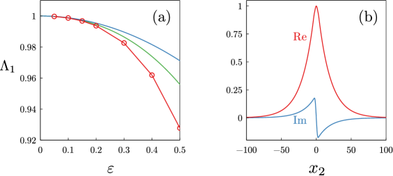
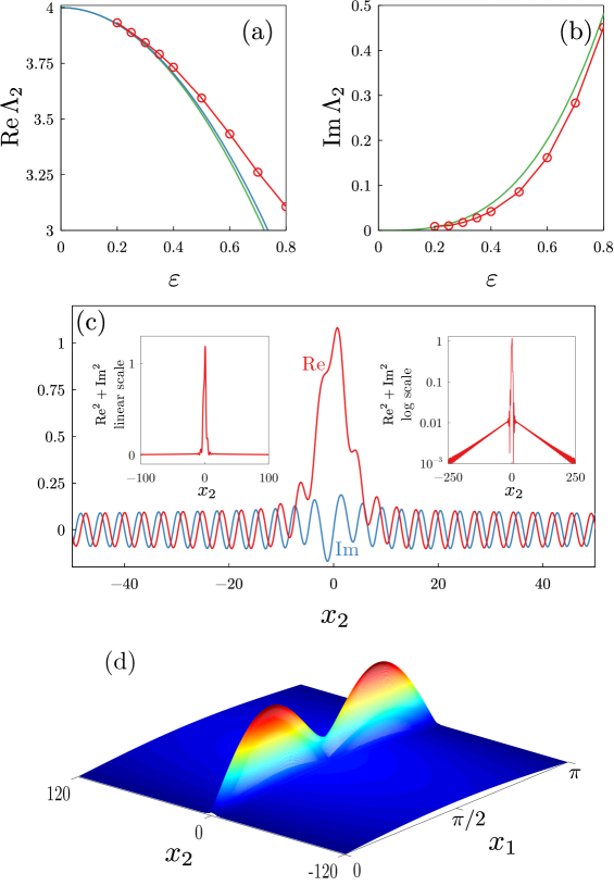
In Fig. 1 we plot the dependencies obtained from the asymptotic expansions, when only the leading term is taken into account and both terms are used, for the particular set of parameters , , . For , the agreement between the analytical predictions and numerical results is rather good, while for large values of it is only qualitative. In Fig. 2 we plot the same data for two eigenvalues bifurcating from the internal threshold with ; here only the eigenvalue with positive imaginary part is shown. The following set of parameters is used: , , , and . Again, the numerical results are in a good agreement with asymptotic expansions for weak perturbations, and in a qualitative agreement for stronger ones. Real part of the eigenvalue is found to decrease with the increase of . Nevertheless, for all values of shown in Fig. 2 the real part of eigenvalue is larger than the lower edge of the essential spectrum. Therefore, in the optical context, the corresponding eigenfunction, whose three-dimensional modulus plot is shown in Fig. 2(d), indeed represents a non-Hermitian generalization of a bound state in the continuum.
3.3.2 Two-dimensional Bose-Einstein condensate with parabolic trapping
In the previous example a choice of was not really important and the discussed results are of a more general nature. For instance, we can choose the operator being a quantum harmonic oscillator. Namely, let and
Then and the operator becomes
As a perturbation, we choose , where is a complex-valued compactly supported potential on . Here
i.e., are Hermite polynomials, and . Then all calculations and results from previous example can be easily reproduced, just in all formulae the functions are to be replaced by the functions introduced above.
The described situation corresponds to a two-dimensional cloud of Bose-Einstein condensate with a parabolic confinement in direction. Assuming that the interparticle interactions are negligible, that is, the condensate is effectively linear, we can model its dynamics by the Schröginer-like equation, which in the theory of Bose-Einstein condensates is known as Gross-Pitaevskii equation [59]:
| (3.12) |
where stands for the macroscopic wavefunction of the condensate. Again, for stationary states in the form , where has the meaning of the chemical potential, the problem is reduced to the described eigenvalue problem. Positive and negative imaginary parts of the perturbation correspond to the injecting the particles from an external source and absorption of the particles, respectively.
3.3.3 Three-dimensional circular waveguide and three-dimensional Bose-Einstein condensate
Here we consider two examples of a three-dimensional waveguide and a three-dimensional quantum oscillator, which extend the above examples of the planar waveguide and the harmonic oscillator adduced above.
In first example we deal with a circular waveguide assuming that and the operator is introduced as the Schrödinger operator with a radially symmetric potential subject to the Dirichlet condition:
Then the domain is a straight cylinder along the axis with the cross-section and
subject to the homogeneous Dirichlet condition. The operator has a purely discrete spectrum and thanks to the assumed radial symmetricity for the potential , it possesses double eigenvalues such that the associated eigenfunctions, orthonormalized in , read as , , where is some fixed integer number, is some real function, and is a polar angle associated with . Such eigenvalues are degenerate internal thresholds in the essential spectrum. We define then a -symmetric potential by formula (3.8) and in addition, we assume that is even in . Then it is easy to see that the corresponding matrix is diagonal:
Then we assume that and , ; these conditions can be easily satisfied by choosing appropriately . Since for both we have , for each corresponding pole we can apply asymptotic expansion (2.44):
where are solutions to the boundary value problem
and can be found by a separation of variables similar to (3.6). Then we can reproduce calculations from the first example and obtain that choosing appropriately the function , we can satisfy conditions (2.27), (2.34) for all poles , , and this means that these poles correspond to eigenvalues. In other words, this means that for appropriately chosen and , we can generate four different simple eigenvalues of the operator in the vicinity of the double eigenvalue of the operator serving as an internal threshold in the essential spectrum.
A similar situation can be realized also in other three-dimensional models. For instance, we can let and , where is some function growing unboundedly at infinity. Such operator again can have double eigenvalues with the eigenfunctions of form and . Linear combinations correspond to vortex states with integer being the vorticity or topological charge. Therefore, in the context of Bose-Einstein condensates, this mechanism can be potentially applied for generation of localized in all three spatial dimensions vortex rings (see e.g. [19]).
We also observe that in both discussed three-dimensional examples the operator can have not only double eigenvalues, but also ones of higher multiplicities . And in such cases, it is possible to find a -symmetric potential generating eigenvalues of the operator in the vicinity of the considered multiple eigenvalue.
4 Meromorphic continuation
In this section we prove Theorem 2.1 on the meromorphic continuation of the resolvent of the operator . First we prove some auxiliary statements in a separate subsection and then we prove the theorem.
4.1 Auxiliary lemmata
In this subsection we prove three auxiliary lemmata, which will be employed in the proof of Theorem 2.1. The first statement is Lemma 2.1.
Proof of Lemma 2.1.
Reproducing literally the proof of Lemma 2.3 in [9], one can check easily the identity . The operator can be represented as a sum of tensor products . And since
we immediately get:
This completes the proof. ∎
The next statement is Lemma 2.2.
Proof of Lemma 2.2.
For each , each and almost each we have:
Hence, the operator maps into . This is an unbounded self-adjoint operator in associated with the restriction of the form on . Moreover, for each we have:
Hence, the spectrum of the operator is located in . The proof is complete. ∎
The third lemma provides a meromorphic continuation for the resolvent of the unperturbed operator.
Lemma 4.1.
Fix and and let be an -multiple eigenvalue of the operator , where . There exists a sufficiently small fixed such that for all complex and all the boundary value problem
| (4.1) |
is solvable in and possesses a solution, which can be represented as
| (4.2) |
where is a linear operator mapping into . This operator is bounded and meromorphic in . It has the only pole in , which is at zero and simple:
| (4.3) | ||||
| (4.4) |
where is an operator bounded uniformly in and holomorphic in , and, we recall, is the operator defined in (2.10).
For sufficiently large , the solution given by (4.2) can be represented as
| (4.5) |
where is some fixed number, are some meromorphic in functions possessing the asymptotic behavior
| (4.6) | ||||||
are some meromorphic in functions, is some fixed constant independent of and , and are some functions meromorphic in and obeying the identities
| (4.7) |
for almost each and for each .
Proof.
The functions
obviously belong to since . It is straightforward to check that the functions
| (4.8) | ||||||
solve the equations
Employing these facts, we seek a solution to problem (4.1) as
| (4.9) |
and for we immediately get problem (4.1) with replaced by the function defined in (2.11). We see easily that .
Thanks to Lemma 2.2, the resolvent is well-defined for all sufficiently small complex provided is small enough. This resolvent is holomorphic in as an operator in and is uniformly bounded in . It can be expanded via the standard Neumann series:
| (4.10) |
This expansion implies that the resolvent is also holomorphic as an operator from into . We define then
and this obviously gives a solution to problem (4.1). We denote the operator mapping into the described solution by and let us show that it possesses all stated properties.
First of all we observe that the introduced operator is independent of the choice of as since in this case the functions with are missing and the above constructions become independent of .
Just by the embeddings and , the resolvent is a bounded operator from into holomorphic in for sufficiently small and bounded uniformly in . An operator mapping into is given explicitly and by straightforward calculations we can check that this is also a bounded operator from into holomorphic in . The calculations are based on estimates of the following kind:
where is some constant independent of . Since the functions belong to , the functions can be expanded into the Laurent series with respect to the small parameter ; in particular, this means that the functionals are well-defined and bounded. Substituting these expansions and (4.10) into (4.9), we immediately get representation (4.3), (4.4), (2.10).
In view of formula (4.9), in order to prove representation (4.5), (4.6), (4.7), it is sufficient to analyze the behavior of the functions at infinity. This can be done easily by an obvious identity
| (4.11) | |||
and an estimate
| (4.12) | ||||
where and are some constants independent of and . The proof is complete. ∎
4.2 Meromorphic continuation for the resolvent of the perturbed operator
This section is devoted to the proof of Theorem 2.1. We begin with rewriting the operator equation
as a boundary value problem (2.3). Then we denote
and rewrite (2.3) as problem (4.1) with the function replaced by . According Lemma 4.1, such problem is solvable and there exists a solution given by formula (4.2):
| (4.13) |
We substitute this formula into corresponding boundary value problem (2.3) and this leads to an operator equation in the space :
Then we substitute representation (4.3), (4.4), (2.10) into this equation:
| (4.14) |
Thanks to the properties of the operators and described in Lemma 4.1, the operator is bounded uniformly in and as an operator in and is holomorphic in . Hence, for sufficiently small , the operator is boundedly invertible and the inverse is holomorphic in as an operator in ; hereinafter the symbol stands for the identity mapping. We denote
| (4.15) |
and apply this operator to equation (4.14). This gives:
| (4.16) |
Our next step is to find . Once we do this, we shall be able to find from equation (4.14) as
| (4.17) |
and recover the function by formula (4.13).
We apply the functionals to equation (4.16) with all such that . As a result, we arrive to a system of linear equations for the vector ; this is a vector-column. The system reads as
| (4.18) |
Here is the unit matrix and is a square matrix with entries , where counts the rows and does the columns in the matrix , while the symbol denotes a vector column with coordinates , . As it was shown in the proof of Lemma 4.1, the functionals are bounded and since the operator is a bounded one in , the introduced matrix and vector are well-defined.
In view of the holomorphy of the operator , the entries of the matrix are holomorphic in and this implies that the matrix is holomorphic in . Hence, the determinant of the matrix is a holomorphic in function and therefore, the matrix is well-defined as a meromorphic in matrix. This allows us to solve system (4.18):
| (4.19) |
where are functionals on meromorphic in . Substituting these formulae into (4.17), we can find and determine by formula (4.13):
| (4.20) | ||||
The function solves problem (2.3) and satisfies representation (2.4), (2.5), (2.6). The latter are implied by similar representations (4.5), (4.6), (4.7) and formula (4.13). Since for sufficiently small the functions , , satisfy asymptotic identities (2.43), the functions , and decay exponentially at infinity as and . Hence, under the same conditions, we have and this means that the operator provides a meromorphic continuation of the resolvent .
We observe that the introduced operator is meromorphic in as an operator from into due to formulae (4.13), (4.17), (4.19) and representation (4.3), (4.4), (2.10).
According to formula (4.20), the poles of the operator defined in this formula coincide with the poles of the functionals . Let at least one of these functionals have a pole at a point . In view of the definition of the functionals in (4.19), this means that the matrix is degenerate and by the Cramer’s rule, system (4.18) with , has a non-trivial solution, which we denote by . We observe that by the definition,
| (4.21) |
Employing these identities and (4.3), (4.4), it is straightforward to check that the formula
| (4.22) | ||||
defines a non-trivial solution to problem (2.3) with , . Thanks to formulae (4.9), (4.8), (4.12), this function can be also represented as
| (4.23) | ||||||
with
and defined by (2.11). We also observe that as , it follows from (4.21) that
for almost each and for each . Representations (4.22), (4.23) and relations (4.11), (4.12) imply representation (2.7), (2.8), (2.9). This completes the proof of Theorem 2.1.
5 Poles of meromorphic continuations
In this section we study the asymptotic behaviour of poles of the operators and we prove Theorems 2.2, 2.3. As it was shown in the proof of Theorem 2.1 in the previous section, the poles of the operator coincides with poles of the matrix . The orders of the mentioned poles of the operator and the orders of the zeroes of obviously coincide.
5.1 Proof of Theorem 2.2
Let us study the solvability of the equation
| (5.1) |
in . It is straightforward to check that
where are some functions holomorphic in and uniformly bounded in and sufficiently small . We fix arbitrary and for sufficiently small we have an uniform estimate:
| (5.2) |
Since on and the function has the only zero in of order at the origin, estimate (5.2) allows us to apply the Rouché theorem and to conclude that equation (5.1) has exactly zeroes counting their orders and these zeroes converge to the origin as .
Our next step is to show that all zeroes of equation (5.1) are located in a ball for some fixed . For arbitrary and sufficiently small such that , by the definition of the function we have:
Then we choose large enough and small enough so that
and applying the Rouché theorem once again, we see that the zeroes of equation (5.1) are located inside the ball . This fact allows us to seek the zeroes of equation (5.1) as , where for all sufficiently small .
The operator defined in (4.15) can be expanded into the standard Neumann series and this yields:
| (5.3) |
In view of the above identity, the change , , and the definition of the matrix , we can represent the latter as
| (5.4) |
where is some uniformly bounded matrix holomorphic in and we recall that the matrix is defined in (2.12). Both these matrices are well-defined since they arise as the terms in the expansion for .
Then we can rewrite equation (5.1) as
| (5.5) |
We recall that , , are different eigenvalues of the matrix of the multiplicities and hence,
This allows us to represent equation (5.5) as
| (5.6) |
where is some function holomorphic in and bounded uniformly in and :
| (5.7) |
By we denote a ball of radius in the complex plane centered at the point . We introduce the balls , where is some fixed number. Then for sufficiently small , each ball contains the only zero of the function , this zero is and the order of this zero is . On the boundary of each ball , for sufficiently small , an obvious estimate holds true:
| (5.8) |
where is some fixed constant independent of and . Hence, in view of estimate (5.7), we can choose large enough and small enough and apply the Rouché theorem to the left hand side of equation (5.6). This yields that each ball contains exactly zeroes of equation (5.6), which we denote by . These zeroes satisfy the asymptotic identities
| (5.9) |
Returning back to equation (5.1), we see that it has exactly zeroes counting their orders and these zeroes obey asymptotic expansion (2.13). The proof is complete.
5.2 Proof of Theorem 2.3
Identity (5.3) allows us to specify the form of the matrix in more details than in (5.4). Namely, this identity implies that
where is some uniformly bounded matrix holomorphic in and we recall that the matrix is defined in (2.14). All these matrices are well-defined as the terms in the expansion for . Equation (5.5) is replaced by a more detailed one:
| (5.10) |
We fix and we are going to study the asymptotic behavior of the zeroes , . Let be a matrix reducing the matrix to its Jordan canonical form, which we denote by . Then equation (5.10) can be rewritten as
Taking into consideration the structure of the matrix , we rewrite this equation as follows:
| (5.11) |
where , are some functions holomorphic in and bounded uniformly in and and is some non-negative integer number. These functions arise as some polynomials in , and the entries of the matrices and . It is clear that , where is defined in (2.15). And if is not identically zero, then
| (5.12) |
where is defined in (2.17). By we denote a ball of radius in the complex plane centered at the point .
We first consider the case, when vanishes identically. Then the term disappears in equation (5.11). Here we consider the ball and for sufficiently small , on the boundary of this ball we have the estimates
where and are some fixed constants independent of and . Then we apply the Rouché theorem proceeding as in (5.6), (5.7), (5.8), (5.9) and we arrive immediately to (2.16).
Now we proceed to the case, when is not identically zero. Here we divide equation (5.11) by and in view of (5.12) we get:
| (5.13) |
where , are some functions holomorphic in in the vicinity of the point and bounded uniformly in and .
Suppose that and consider the ball . For sufficiently small , on the boundary of this ball we have
| (5.14) | ||||
and
| (5.15) |
where is some constant independent of and . Since , it is also straightforward to check that for sufficiently small and sufficiently large , all zeroes of the function belong to the ball . Taking this fact and estimates (5.14), (5.15) into consideration, we apply the Rouché theorem and arrive at asymptotic expansion (2.18).
Suppose that . The zeroes of the function can be found explicitly. The first of them is a -multiple zero and simple zeroes
| (5.16) |
First we consider a ball and we observe that under our assumption, . Hence, for sufficiently small , the ball does not contain the zeroes . Moreover, on the boundary of this ball, the estimate holds true:
We also observe that estimate (5.15) remains true in the considered case. Then we apply Rouché theorem to the ball and conclude that this ball contains exactly zeroes of equation (5.13) counting their orders. This implies asymptotic expansion (2.19).
Now we consider another ball for defined in (5.16) with some fixed . For sufficiently small , this ball does not contain the origin and other points with . On the boundary of this ball, we have the following estimate:
| (5.17) | ||||
where is some constant independent of and . We observe that under our assumptions
In view of the latter inequality, on the boundary of the ball , the estimates
hold true, where is some constant independent of and . This estimate and (5.17) allow us to apply the Rouché theorem and we conclude that the ball contains exactly one zero of equation (5.11). This gives asymptotic expansion (2.20). The proof is complete.
6 Emerging resonances and eigenvalues
In this section we determine whether the poles of the operators described in the previous section correspond to the eigenvalues or resonances of the operator . In this way, we shall prove Theorems 2.4, 2.5.
We fix and assume that , where is a multiplicity of the eigenvalue of the operator . In what follows, we analyze the nature of poles from Theorem 2.2 with asymptotic behavior (2.13). In order to do this, we analyze the behavior of the associated nontrivial solutions to problem (2.3) with .
6.1 Bottom of the spectrum
In this subsection we assume that and we prove Theorem 2.4. In the considered case, the meromorphic continuation of the resolvent given the operator is independent of and the same is true for the corresponding poles from Theorem 2.2 with asymptotic behavior (2.13). The behavior of the associated nontrivial solutions to problem (2.3) with is provided by representation (2.7). In this representation, the first sum over is obviously missing and the leading term at infinity is the sum over .
We fix one of the poles with some , . It follows from (4.21), (4.22), (4.23), (4.3), (4.4) that the coefficients , , in representation (2.7) coincide with determined by (4.21). Since we deal with a non-trivial solution of system (4.21), this implies that at least one of the coefficients is non-zero. Then representation (2.7) for a non-trivial solution to problem (2.3) defined in (4.22) and formulae (2.43) imply that if
| (6.1) |
then a non-trivial solution decays exponentially at infinity and thus, is an eigenfunction, while the opposite inequality
| (6.2) |
ensures that is not in .
Asymptotic expansions for established in Theorems 2.2, 2.3 allow us to check effectively the above conditions. Namely, if , this ensures inequality (6.1) for sufficiently small . Then the poles , correspond to the eigenvalues with asymptotic expansions (2.21), (2.22), (2.23) as described in the formulation of Theorem 2.4. If , this guarantees inequality (6.2) for sufficiently small and the poles correspond to the resonances with same asymptotic expansions (2.21), (2.22), (2.23).
If , in order to understand which of conditions (6.1), (6.2) is realized, we need to check the next term in the asymptotic expansion for . According Theorem 2.3, this can be done under an additional assumption and only for poles with . Then asymptotic expansion (2.20) imply that under condition (2.24), the pole , corresponds to an eigenvalue, while under condition (2.25) the pole corresponds to a resonance. The asymptotic behavior for this eigenvalue/resonance is given by (2.23) if and it is given by (2.26) if .
6.2 Internal thresholds in the spectrum
In this subsection we study the nature of the poles emerging from internal points in the essential spectrum and we prove Theorem 2.5. As in the previous subsection, here we again analyze the behavior at infinity of non-trivial solutions associated with poles and this analysis will be based on representation (2.7). However, there are important differences. The matter is that now the representation involves also a sum over . Its terms can decay or grow at infinity. As it has been mentioned in the proof of Theorem 2.1, according identity (2.43), the functions , , decay exponentially at infinity if and grow exponentially or vary periodically as . This means that apart of the sign of , we should also control the sign of . One more point is that now we have two meromorphic continuations of the resolvent, the operators , , respectively, two sets of their poles converging to zero as . We observe that according Theorems 2.2, 2.3, the first terms in asymptotic expansions for poles are the eigenvalues of the matrix and they are independent of . In fact, we can see the influence of on the asymptotic behavior of only in formulae (2.20), for under an additional assumption .
We choose , , and consider the pole . As in the above proof of Theorem 2.4, it is easy to see that at least one of the coefficients , , in representation (2.7) for the associated non-trivial functions is non-zero. Then it follows from asymptotic expansions (2.16), (2.18), (2.19), (2.20) that conditions (2.27), (2.30), (2.31), (2.34) ensure that and and hence, the pole corresponds to an eigenvalue . The stated asymptotic behavior for this eigenvalue is implied by (2.16), (2.18), (2.19), (2.20). In the same way, conditions (2.35), (2.38) ensure that and hence, the pole corresponds to a resonance and it possesses the stated behavior.
If is a simple eigenvalue of the matrix , then . In this case, a non-trivial solution to system (4.21) associated with converges to the vector . Indeed, it follows from representation (5.4) that the corresponding zero of equation (5.5) is an eigenvalue of the matrix and is an associated eigenvector. And since converges to and both these eigenvalues are simple, the eigenvector associated with converges to as well. Now by representation (4.22), (4.23), definition (2.10) of the operator and formula (4.11) we conclude that the coefficients in representation (2.7) satisfy the identities:
Hence, by condition (2.42), at least one of the coefficients is non-zero. As above, it is easy to see that one of conditions (2.27) or (2.30) and one of conditions (2.39) or (2.41) ensures that the functions grows exponentially at infinity and hence, the same is true for the function . Therefore, the pole corresponds to a resonance. The asymptotic expansion for this resonance can be established as above. The proof of Theorem 2.5 is complete.
Acknowledgments
The authors thank the referees for useful remarks. The research by D.I.B. and D.A.Z. is supported by the Russian Science Foundation (Grant No. 20-11-19995).
Data Availability Statement
The data that support the findings of this study are available from the corresponding author upon reasonable request.
References
- [1] I.V. Barashenkov, D.A. Zezyulin and V.V. Konotop, Jamming anomaly in -symmetric systems, New J. Phys. 18 (2016) 075015.
- [2] C.M. Bender, Making sense of non-Hermitian Hamiltonians, Rep. Prog. Phys. 70 (2007) 947–1018.
- [3] C.M. Bender and S. Boettcher, Real spectra in non-Hermitian Hamiltonians having -symmetry, Phys. Rev. Lett. 80 (1998) 5243–5246.
- [4] R. Blankenbecler, M. L. Goldberger, B. Simon, The bound states of weakly coupled long-range one-dimensional quantum Hamiltonians, Ann. Physics, 108(1977) 69–78.
- [5] D. Borisov, Discrete spectrum of a pair of non-symmetric waveguides coupled by a window, Sb. Math., 197 (2006) 475–504.
- [6] D. Borisov, Asymptotic behaviour of the spectrum of a waveguide with distant perturbation, Math. Phys. Anal. Geom. 10 (2007) 155–196.
- [7] D.I. Borisov, Distant perturbations of the Laplacian in a multi-dimensional space, Ann. H. Poincaré, 8 (2007) 1371–1399.
- [8] D.I. Borisov, R.R. Gadyl’shin, On spectrum of periodic operator with a small localized perturbation, Izv. Math. 72 (2008) 659–688.
- [9] D. Borisov, On spectrum of two-dimensional periodic operator with small localized perturbation, Izv. Math. 75 (2011) 471–505.
- [10] D. Borisov, S. Dmitriev, On the spectral stability of kinks in 2D Klein-Gordon model with parity-time-symmetric perturbation, Stud. Appl. Math. 138 (2017) 317–342.
- [11] D. Borisov, G. Cardone, On a one-dimensional quadratic operator pencil with a small periodic perturbation, ESAIM: COCV 26 (2020) id 21.
- [12] D. Borisov, D. Krejčiřík, -symmetric waveguide, Integ. Equat. Oper. Theo. 62 (2008) 489–515.
- [13] D. Borisov, Emergence of eigenvalue for -symmetric operator in thin strip, Math. Notes. 98 (2015) 827–883.
- [14] D.I. Borisov, M. Znojil, On eigenvalues of a -symmetric operator in a thin layer, Sb. Math. 208 (2017) 173–199.
- [15] D. Borisov, The spectrum of two quantum layers coupled by a window, J. Phys. A: Math. Theor. 40 (2007) 5045–5066.
- [16] D. Borisov, Perturbation of threshold of essential spectrum for waveguide with window. I. Decaying resonance solutions, J. Math. Sci. 205 (2015) 19–54.
- [17] D.I. Borisov, D.A. Zezyulin, Spacing gain and absorption in a simple PT-symmetric model: spectral singularities and ladders of eigenvalues and resonances, J. Phys. A: Math. Theor. 52 (2019) id 445202.
- [18] D.I. Borisov, D.A. Zezyulin, Sequences of closely spaced resonances and eigenvalues for bipartite complex potentials, Appl. Math. Lett. 100 (2020) id 106049.
- [19] L. D. Carr and J. Brand, Multidimensional solitons: theory, in Emergent nonlinear phenomena in Bose-Einstein condensates: theory and experiment, ed. by P. G. Kevrekidis, D. J. Frantzeskakis, and R. Carretero-González (Springer, Berlin, 2008).
- [20] S. Cuccagna, D. Pelinovsky, Bifurcations from the endpoints of the essential spectrum in the linearized nonlinear Schrödinger problem, J. Math. Phys. 46 (2005) 053520.
- [21] P. Duclos and P. Exner, Curvature-induced bound state in quantum waveguides in two and three dimensions, Rev. Math. Phys. 7 (1995) 73–102.
- [22] R. El-Ganainy, K.G. Makris, M. Khajavikhan, Z.H. Musslimani, S. Rotter and D.N. Christodoulides, Non-Hermitian physics and PT symmetry, Nat. Phys. 14 (2018) 11–19.
- [23] P. Exner, P. Šeba, M. Tater, D. Vaněk, Bound states and scattering in quantum waveguides coupled laterally through a boundary window, J. Math. Phys. 37 (1996) 4867–4887.
- [24] L. Feng, R. El-Ganainy, and L. Ge, Non-hermitian photonics based on parity-time symmetry, Nat. Photonics 11 (2017) 752–762.
- [25] R.R. Gadyl’shin, Local perturbations of the Schrödinger operator on the axis, Theor. Math. Phys. 132 (2002) 976–-982.
- [26] R. R. Gadyl’shin, Local perturbations of the Schrödinger operator on the plane, Theor. Math. Phys. 138 (2004), 33–44.
- [27] R.R. Gadyl’shin. On regular and singular perturbations of acoustic and quantum waveguides, C.R. Méch. 332 (2004) 647–652.
- [28] S. Garmon, M. Gianfreda, and N. Hatano, Bound states, scattering states, and resonant states in -symmetric open quantum systems, Phys. Rev. A 92, (2015) id 022125.
- [29] F. Gesztesy, H. Holden, A unified approach to eigenvalues and resonances of Schrödinger operators using Fredholm determinants, J. Math. Anal. Appl. 123 (1987) 181–198.
- [30] W.D. Heiss, The physics of exceptional points, J. Phys. A: Math. Theor. 45 (2011) id 444016.
- [31] R. Høegh-Krohn, M. Mebkhout, The expansion for the critical multiple well problem, Comm. Math. Phys. 91 (1983) 65–73.
- [32] C. W. Hsu, B. Zhen, A. Douglas Stone, J. D. Joannopoulos M. Soljačić, Bound states in the continuum, Nat. Rev. Mater. 1(2016), 16048.
- [33] N.N. Kalitkin, A.B. Alshin, Ye.A. Alshina, B.V. Rogov, Calculations On Quasi-Equidistant Grids, (Fizmatlit 2005). (in Russian)
- [34] Y. V. Kartashov, C. Milián, V. V. Konotop, and L. Torner, Bound states in the continuum in a two-dimensional PT-symmetric system, Opt. Lett. 43, (2018) 575–578.
- [35] T. Kato, Perturbation Theory for Linear Operators, (Springer-Verlag, 1976).
- [36] Yu. S. Kivshar, G. P. Agrawal, Optical Solitons: From Fibers to Photonic Crystals, (Academic Press, 2003).
- [37] M. Klaus, On the bound state of Schrödinger operators in one dimension, Ann. Phys. 108 (1977), 288–-300.
- [38] M. Klaus, B. Simon, Coupling constant thresholds in nonrelativistic quantum mechanics. I. Short-range two-body case, Ann. Phys. 130 (1980) 251–281.
- [39] K. Knopp, Theory of functions. Part II. (Dover Publ. 1947).
- [40] V. V. Konotop, J. Yang, D. A. Zezyulin, Nonlinear waves in -symmetric systems, Rev. Mod. Phys. 88 (2016) id 035002.
- [41] V. V. Konotop and D. A. Zezyulin, Phase transition through the splitting of self-dual spectral singularity in optical potentials, Opt. Lett. 42 (2017) 5206–5209.
- [42] V. V. Konotop and D. A. Zezyulin, Spectral singularities of odd--symmetric potentials, Phys. Rev. A 99 (2019) 013823.
- [43] S. Longhi, Parity-time symmetry meets photonics: A new twist in non-hermitian optics. Europhys. Lett. 120 (2017) id 64001.
- [44] S. Longhi, Bound states in the continuum in -symmetric optical lattices, Opt. Lett. 39 (2014) 1697–1700.
- [45] C. Meng, X. Zhang, S. T. Tang, M. Yang, Z. Yang, Acoustic coherent perfect absorbers as sensitive null detectors, Sci. Rep. 7 (2017) id 43574
- [46] M.-A. Miri and A. Alú, Exceptional points in optics and photonics, Science 363 (2019) eaar7709.
- [47] N. Moiseyev, Non-Hermitian Quantum Mechanics (Cambridge Univ. Press, 2011).
- [48] A. Mostafazadeh, Pseudo-hermitian Representation of Quantum Mechanics. Int. J. Geom. Methods Mod. Phys. 7 (2010) 1191–1306.
- [49] A. Mostafazadeh, Spectral singularities of complex scattering potentials and infinite reflection and transmission coefficients at real energies Phys. Rev. Lett. 102 (2009) id 220402.
- [50] A. Mostafazadeh, Physics of spectral singularities, Trends in Mathematics 145 (Springer International Publishing, 2015).
- [51] J. G. Muga, J. P. Palao, B. Navarro, and I. L. Egusquiza, Complex absorbing potentials, Phys. Rep. 395 (2004) 357–426.
- [52] A. Müllers, B. Santra, C. Baals, J. Jiang, J. Benary, R. Labouvie, D. A. Zezyulin, V. V. Konotop, H. Ott, Coherent perfect absorption of nonlinear matter waves. Sci. Adv. 4 (2018) eaat6539.
- [53] M. A. Naimark, Investigation of the spectrum and the expansion in eigenfunctions of a nonselfadjoint operator of the second order on a semi-axis, Tr. Mosk. Mat. Obs. 3 (1954) 181–270.
- [54] S.A. Nazarov, Almost standing waves in a periodic waveguide with a resonator and near-threshold eigenvalues, St. Petersburg Math. J. 28 (2017) 377–410.
- [55] S.A. Nazarov, Threshold resonances and virtual levels in cylindrical and periodic waveguides, Izv. Math. 84 (2020), to appear. DOI: 10.1070/IM8928
- [56] J. von Neumann and E. Wigner, Über merkwürdige diskrete eigenwerte, Phys. Z. 30 (1929) 467–470.
- [57] Ş. K. Özdemir, S. Rotter, F. Nori, and L. Yang, Parity-time symmetry and exceptional points in photonics, Nature Materials 18 (2019) 783–798.
- [58] J. Pappademos, U. Sukhatme, and A. Pagnamenta, Bound states in the continuum from supersymmetric quantum mechanics, Phys. Rev. A 48 (1993) 3525–3532.
- [59] L.P. Pitaevskii and S. Stringari, Bose-Einstein Condensation, (Clarendon Press, 2003).
- [60] M. Robnik, A simple separable Hamiltonian having bound states in the continuum, J. Phys. A: Math. Gen. 19 (1986) 3845–3848.
- [61] J. Schwartz, Some non-selfadjoint operators, Comm. Pure Appl. Math. 13 (1960) 609–639.
- [62] B. Simon, The bound state of weakly coupled Schrödinger operators in one and two dimensions, Ann. Phys. 97 279–288 (1976).
- [63] F. H. Stillinger and D. R. Herrick, Bound states in the continuum, Phys. Rev. A 11 (1975) 446–454.
- [64] B. Vainberg, On the analytical properties of the resolvent for a certain class of operator-pencils, Math. USSR Sbornik 6 (1968) 241–273.
- [65] V. Vougalter, On threshold eigenvalues and resonances for the linearized NLS equation, Math. Model. Nat. Phenom. 5 (2010), no. 4, 448-469.
- [66] W. Wan, Y. Chong, L. Ge, H. Noh, A. D. Stone, H. Cao, Time-reversed lasing and interferometric control of absorption, Science 331 (2011) 889–892.
- [67] J. Yang, Classes of non-parity-time-symmetric optical potentials with exceptional-point-free phase transitions, Opt. Lett. 42 (2017) 4067–4070.
- [68] J. Yang, Partially -symmetric optical potentials with all-real spectra and soliton families in multidimensions, Opt. Lett. 39 (2014) 1133–1136.
- [69] V. A. Zheludev, Perturbations of the spectrum of the Schrödinger operator with a complex periodic potential, Spectral Theory, Topics Math. Phys. 3 (1969) 25–41.
- [70] A. A. Zyablovsky, A.P. Vinogradov, A.A. Pukhov, A.V. Dorofeenko and A.A. Lisyansky, -symmetry in optics, Physics – Uspekhi (2014) 57 1063–1082.