66email: jan.huisken@uni-goettingen.de, tingying.peng@helmholtz-muenchen.de
BigFUSE: Global Context-Aware Image Fusion in Dual-View Light-Sheet Fluorescence Microscopy with Image Formation Prior
Abstract
Light-sheet fluorescence microscopy (LSFM), a planar illumination technique that enables high-resolution imaging of samples, experiences “defocused” image quality caused by light scattering when photons propagate through thick tissues. To circumvent this issue, dual-view imaging is helpful. It allows various sections of the specimen to be scanned ideally by viewing the sample from opposing orientations. Recent image fusion approaches can then be applied to determine in-focus pixels by comparing image qualities of two views locally and thus yield spatially inconsistent focus measures due to their limited field-of-view. Here, we propose BigFUSE, a global context-aware image fuser that stabilizes image fusion in LSFM by considering the global impact of photon propagation in the specimen while determining focus-defocus based on local image qualities. Inspired by the image formation prior in dual-view LSFM, image fusion is considered as estimating a focus-defocus boundary using Bayes’ Theorem, where (i) the effect of light scattering onto focus measures is included within Likelihood; and (ii) the spatial consistency regarding focus-defocus is imposed in Prior. The expectation-maximum algorithm is then adopted to estimate the focus-defocus boundary. Competitive experimental results show that BigFUSE is the first dual-view LSFM fuser that is able to exclude structured artifacts when fusing information, highlighting its abilities of automatic image fusion.
Keywords:
Light-sheet Fluorescence Microscopy (LSFM) Multi-View Image Fusion Bayesian.1 Introduction
Light-sheet fluorescence microscopy (LSFM), characterized by orthogonal illumination with respect to detection, provides higher imaging speeds than other light microscopies, e.g., confocal microscopy, via gentle optical sectioning [14, 15, 5], which makes it well-suited for whole-organism studies [11]. At macroscopic scales, however, light scattering degrade image quality. It leads to images from deeper layers of the sample being of worse quality than from tissues close to the illumination source [17, 6]. To overcome the negative effect of photon propagation, dual-view LSFM is introduced, in which the sample is sequentially illuminated from opposing directions, and thus portions of the specimen with inferior quality in one view will be better in the other [16] (Fig. 1a). Thus, image fusion methods that combine information from opposite views into one volume are needed.
To realize dual-view LSFM fusion, recent pipelines adapt image fusers for natural image fusion to weigh between views by comparing the local clarity of images [16, 17]. For example, one line of research estimates focus measures in a transformed domain, e.g., wavelet [7] or contourlet [18], such that details with various scales can be considered independently [10]. However, the composite result often exhibits global artifacts [8]. Another line of studies conducts fusion in the image space, with pixel-level focus measures decided via local block-based representational engineerings such as multi-scale weighted multi-scale weighted gradient [20] and SIFT [9]. Unfortunately, spatially inconsistent focus measures are commonly derived for LSFM, considering the sparse structures of the biological sample involved by the limited field-of-view (FOV).
Apart from limited FOV, another obstacle that hinders the adoption of natural image fusion methods into dual-view LSFM is the inability to distinguish sample structures from structural artifacts [1]. For example, ghost artifacts, surrounding the sample as a result of scattered illumination light [3], can be observed, as it only appears in regions far from the light source after light travels through scattering tissues. Yet, when ghosts appear in one view, the same region in the opposite view would be background, i.e., no signal. Thus, ghosts will be erroneously transferred to the result by conventional fusion studies, as they are considered as owning richer information than its counterpart in the other view.
Here, we propose BigFUSE to realize spatially consistent image fusion and exclude ghost artifacts. Main contributions are summarized as follows:
-
BigFUSE is the first effort to think of dual-view LSFM fusion using Bayes, which maximizes the conditional probability of fused volume regarding image clarity, given the image formation prior of opposing illumination directions.
-
The overall focus measure along illumination is modeled as a joint consideration of both global light scattering and local neighboring image qualities in the contourlet domain, which, together with the smoothness of focus-defocus, can be maximized as Likelihood and Prior in Bayesian.
-
Aided by a reliable initialization, BigFUSE can be efficiently optimized by utilizing expectation-maximum (EM) algorithm.
2 Methods
An illustration of BigFUSE for dual-view LSFM fusion is given in Fig. 1. First, pixel-level focus measures are derived for two opposing views separately, using nonsubsampled contourlet transform (NSCT) (Fig. 1b). Pixel-wise photon propagation maps in tissue are then determined along light sheet via segmentation (Fig. 1c). The overall focus measures are thus modeled as the inverse of integrated photon scattering along illumination conditioned on the focus-defocus change, i.e., Likelihood, whereas the smoothness of focus-defocus is ensured via Prior. Finally, the focus-defocus boundary is optimized via EM (Fig. 1d).
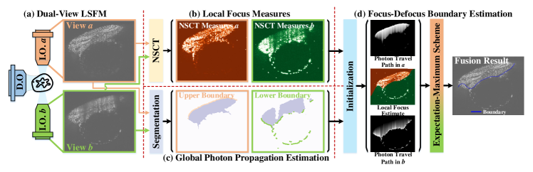
2.1 Revisiting Dual-View LSFM Fusion using Bayes
BigFUSE first rethinks dual-view LSFM fusion from a Bayesian perspective, that is, the conditional probability of fused volume in terms of ”in-focusness”, is given on not only a pair of image inputs, but also prior knowledge that these two images are illiminated from opposing orientations respectively:
| (1) |
where is our predicted fusion with minimal light scattering effect. and are two image views illuminated by light source and , respectively. We choose depending on their competitive image clarity at each pixel. Priors denote our empirical favor of against at each pixel if photons travel through fewer scattering tissues from source a than b, and vice versa. Due to the non-positive light scattering effect along illumination path, there is only one focus-defocus change per column for dual-view LSFM in Fig. 1a. Thus, fusion is equivalent to estimating a focus-defocus boundary defined as a function associating focus-defocus changes to column indexes:
| (2) |
which can be further reformulated by logarithm:
| (3) | |||||
where denotes the focus-defocus changeover at i-th column, is the i-th column of . Next, estimating is decomposed into: (i) define the column-wise image clarity, i.e., log-likelihood ; (ii) consider the belief on a spatially smooth focus-defocus boundary, namely log-prior .
2.2 Image Clarity Characterization with Image Formation Prior
In LSFM, log-likelihood can be interpreted as the probability of observing given the hypothesis that the focus-defocus change is determined as in the i-th column:
| (4) |
where is a concatenation, is the columne-wise image clarity to be defined.
2.2.1 Estimating Pixel-Level Image Clarity in NSCT.
To define , BigFUSE first uses NSCT, a shift-invariant image representation technique, to estimate pixel-level focus measures by characterizing salient image structures [18]. Specifically, NSCT coefficients and are derived for two opposing LSFM views, where , is the lowpass coefficient at the coarsest scale, is the bandpass directional coefficient at i-th scale and l-th direction. Local image clarity is then projected from and [18]:
| (5) |
where is local directional band-limited image contrast and is the smoothed image baseline, whereas highlights image features that are distributed only on a few directions, which is helpful to exclude noise [18]. As a result, pixel-level image clarity is quantified for respective LSFM view.
2.2.2 Reweighting Image Clarity Measures by Photon Traveling Path.
Pixel-independent focus measures may be adversely sensitive to noise, due to the limited receptive field when characterizing local image clarities. Thus, BigFUSE proposes to integrate pixel-independent image clarity measures along columns by taking into consideration the photon propagation in depth. Specifically, given a pair of pixels , is empirically more in-focus than , if photons travel through fewer light-scattering tissues from illumination objective a than from b to get to position (m, n), and vice versa. Therefore, BigFUSE defines column-level image clarity measures as:
| (6) |
where is to model the image deterioration due to light scattering. To visualize photon traveling path, BigFUSE uses OTSU thresholding for foreground segmentation (followed by AlphaShape to generalize bounding polygons), and thus obtains sample boundary, i.e., incident points of light sheet, which we refer to as and for opposing views a and b respectively. Since the derivative of implicitly refers to the spatially varying index of refraction within the sample, which is nearly impossible to accurately measure from the physics perspective, we model it using a piecewise linear model, without loss of generality:
| (10) |
As a result, is obtained as summed pixel-level image clarity measures with integral factors conditioned on photon propagation in depth.
2.3 Least Squares Smoothness of Focus-Defocus Boundary
With log-likelihood considering the focus-defocus consistency along illuminations using image formation prior in LSFM, BigFUSE then ensures consistency across columns in . Specifically, the smoothness of is characterized as a window-based polynomial fitness using linear least squares:
| (11) |
where , , is the parameters to be estimated, the sliding window is with a size of .
2.4 Focus-Defocus Boundary Inference via EM
Finally, in order to estimate the together with the fitting parameter , BigFUSE reformulates the the posterior distribution in Eq. (2) as follows:
| (12) |
where is the trade-off parameter. Here, BigFUSE alternates the estimations of , and , and iterates until the method converges. Specifically, given for the n-th iteration, is estimated by maximizing (E-step):
| (13) |
which can be solved by iterating over . BigFUSE then updates based on least squares estimation:
| (14) |
Additionally, is updated based on Eq. (10) subject to (M-step). BigFUSE proposes to initialize based on and :
| (15) |
where denotes the total number of elements in .
2.5 Competitive Methods
We compare BigFUSE to four baseline methods: (i) DWT [16]: a multi-resolution image fusion method using discrete wavelet transform (DWT); (ii) NSCT [18]: another multi-scale image fuser but in the NSCT domain; (iii) dSIFT [9]: a dense SIFT-based focus estimator in the image space; (iv) BF [19]: a focus-defocus boundary detection method that considers region consistency in focus; and two BigFUSE variations: (v) : built by disabling smooth constraint; (vi) : formulated by replacing the weighted summation of pixel-level clarity measures for overall characterization, by a simple average.
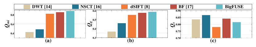
To access the blind image fusion performance, we adopt three fusion quality metrics, [4], [12] and [13]. Specifically, , and use mutual information, gradient or image quality index to quantify how well the information or features of the inputs are transferred to the result, respectively. In the simulation studies where ground truth is available, mean square error (EMSE) and structural similarity index (SSIM) are used for quantification.
[b] DWT [16] NSCT [18] dSIFT [9] BF [19] BigFUSE EMSE () 6.81 0.72 4.66 0.56 5.17 0.72 1.55 0.25 1.43 0.34 0.96 0.08 0.94 0.09 SSIM 0.974 0.02 0.996 0.03 0.93 0.01 0.994 0.03 0.993 0.02 0.993 0.02 . 0.998 0.01
3 Results and Discussion
3.1 Evaluation on LSFM Images with Synthetic Blur
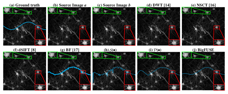
We first evaluate BigFUSE in fusing dual-view LSFM blurred by simulation. Here, we blur a mouse brain sample collected in [2] with spatially varying Gaussian filter for thirty times, which is chemically well-cleared and thus provides an almost optimal ground truth for simulation, perform image fusion, and compare the results to the ground truth. BigFUSE achieves the best EMSE and SSIM, statistically surpassing other approaches (Table. 1, using Wilcoxon signed-rank test). Only BigFUSE and BF realize information fusing without damaging original images with top two EMSE. In comparison, DWT, NSCT and dSIFT could distort the original signal when fusing (green box in Fig. 2).
3.2 Evaluation on LSFM Images with Real Blur
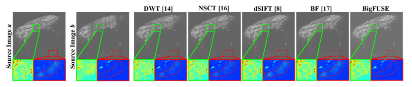
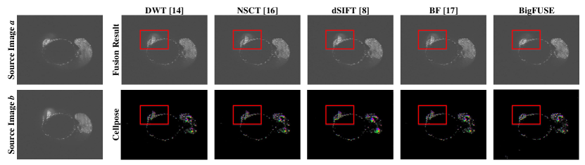
BigFUSE is then evaluated against baseline methods on real dual-view LSFM. A large sample volume, zebrafish embryo ( for each view), is imaged using a Flamingo Light Sheet Microscope. BigFUSE takes roughly nine minutes to process this zebrafish embryo, using a T4 GPU with 25 GB system RAM and 15 GB GPU RAM. In Fig. 4, inconsistent boundary is detected by BF, while methods like DWT and NSCT generate structures that do not exist in either input. Moreover, only BigFUSE can exclude ghost artifact from the result (red box), as BigFUSE is the only pipeline that considers image formation prior. Additionally, we demonstrate the impact of bigFUSE on a specific downstream task in Fig. 5, i.e., segmentation by Cellpose. Only the fusion result provided by bigFUSE allows reasonable predicted cell pose, given that ghosting artifacts are excluded dramatically. This explains why the in Fig. 3 is suboptimal, since BigFUSE do not allow for the transmission of structural ghosts to the output.
4 Conclusion
In this paper, we propose BigFUSE, a image fusion pipline with image formation prior. Specifically, image fusion in dual-view LSFM is revisited as inferring a focus-defocus boundary using Bayes, which is essential to exclude ghost artifacts. Furthermore, focus measures are determined based on not only pure image representational engineering in NSCT domain, but also the empirical effects of photon propagation in depth embeded in the opposite illumination directions in dual-view LSFM. BigFUSE can be efficiently optimized using EM. Both qualitative and quantitative evaluations show that BigFUSE surpasses other state-of-the-art LSFM fusers by a large margin. BigFUSE will be made accessible.
4.0.1 Acknowledgements
Y.L. is supported by the China Scholarship Council (No. 202106020050). J.H. is funded by the Alexander von Humboldt Foundation in the framework of the Alexander von Humboldt Professorship endowed by the German Federal Ministry of Education and Research and funded by the Deutsche Forschungsgemeinschaft (DFG, German Research Foundation) under Germany’s Excellence Strategy - EXC 2067/1- 390729940.
References
- [1] Azam, M.A., Khan, K.B., Salahuddin, S., Rehman, E., Khan, S.A., Khan, M.A., Kadry, S., Gandomi, A.H.: A review on multimodal medical image fusion: Compendious analysis of medical modalities, multimodal databases, fusion techniques and quality metrics. Computers in Biology and Medicine 144, 105253 (2022). https://doi.org/https://doi.org/10.1016/j.compbiomed.2022.105253
- [2] Dean, K.M., Chakraborty, T., Daetwyler, S., Lin, J., Garrelts, G., M’Saad, O., Mekbib, H.T., Voigt, F.F., Schaettin, M., Stoeckli, E.T., et al.: Isotropic imaging across spatial scales with axially swept light-sheet microscopy. Nature protocols 17(9), 2025–2053 (2022). https://doi.org/10.1038/s41596-022-00706-6
- [3] Fahrbach, F.O., Simon, P., Rohrbach, A.: Microscopy with self-reconstructing beams. Nature photonics 4(11), 780–785 (2010). https://doi.org/10.1038/nphoton.2010.204
- [4] Hossny, M., Nahavandi, S., Creighton, D.: Comments on’information measure for performance of image fusion’ (2008)
- [5] Keller, P.J., Stelzer, E.H.: Quantitative in vivo imaging of entire embryos with digital scanned laser light sheet fluorescence microscopy. Current opinion in neurobiology 18(6), 624–632 (2008). https://doi.org/10.1016/j.conb.2009.03.008
- [6] Krzic, U., Gunther, S., Saunders, T.E., Streichan, S.J., Hufnagel, L.: Multiview light-sheet microscope for rapid in toto imaging. Nature methods 9(7), 730–733 (2012). https://doi.org/10.1038/nmeth.2064
- [7] Lewis, J.J., O’Callaghan, R.J., Nikolov, S.G., Bull, D.R., Canagarajah, N.: Pixel-and region-based image fusion with complex wavelets. Information fusion 8(2), 119–130 (2007). https://doi.org/10.1016/j.inffus.2005.09.006
- [8] Li, S., Kang, X., Hu, J.: Image fusion with guided filtering. IEEE Transactions on Image processing 22(7), 2864–2875 (2013). https://doi.org/10.1109/TIP.2013.2244222
- [9] Liu, Y., Liu, S., Wang, Z.: Multi-focus image fusion with dense sift. Information Fusion 23, 139–155 (2015). https://doi.org/10.1016/j.inffus.2014.05.004
- [10] Liu, Y., Wang, L., Cheng, J., Li, C., Chen, X.: Multi-focus image fusion: A survey of the state of the art. Information Fusion 64, 71–91 (2020). https://doi.org/https://doi.org/10.1016/j.inffus.2020.06.013
- [11] Medeiros, G.d., Norlin, N., Gunther, S., Albert, M., Panavaite, L., Fiuza, U.M., Peri, F., Hiiragi, T., Krzic, U., Hufnagel, L.: Confocal multiview light-sheet microscopy. Nature communications 6(1), 8881 (2015). https://doi.org/10.1038/ncomms9881
- [12] Petrovic, V., Xydeas, C.: Objective image fusion performance characterisation. In: Tenth IEEE International Conference on Computer Vision (ICCV’05) Volume 1. vol. 2, pp. 1866–1871. IEEE (2005). https://doi.org/10.1109/ICCV.2005.175
- [13] Piella, G., Heijmans, H.: A new quality metric for image fusion. In: Proceedings 2003 international conference on image processing (Cat. No. 03CH37429). vol. 3, pp. III–173. IEEE (2003). https://doi.org/10.1109/ICIP.2003.1247209
- [14] Power, R.M., Huisken, J.: A guide to light-sheet fluorescence microscopy for multiscale imaging. Nature methods 14(4), 360–373 (2017). https://doi.org/10.1038/nmeth.4224
- [15] Reynaud, E.G., Peychl, J., Huisken, J., Tomancak, P.: Guide to light-sheet microscopy for adventurous biologists. Nature methods 12(1), 30–34 (2015). https://doi.org/10.1038/nmeth.3222
- [16] Rubio-Guivernau, J.L., Gurchenkov, V., Luengo-Oroz, M.A., Duloquin, L., Bourgine, P., Santos, A., Peyrieras, N., Ledesma-Carbayo, M.J.: Wavelet-based image fusion in multi-view three-dimensional microscopy. Bioinformatics 28(2), 238–245 (2012). https://doi.org/10.1093/bioinformatics/btr609
- [17] Verveer, P.J., Schoonderwoert, V.T., Ressnikoff, D., Elliott, S.D., van Teutem, K.D., Walther, T.C., van der Voort, H.T.: Restoration of light sheet multi-view data with the huygens fusion and deconvolution wizard. Microscopy today 26(5), 12–19 (2018). https://doi.org/10.1017/S1551929518000846
- [18] Zhang, Q., Guo, B.l.: Multifocus image fusion using the nonsubsampled contourlet transform. Signal processing 89(7), 1334–1346 (2009). https://doi.org/10.1016/j.sigpro.2009.01.012
- [19] Zhang, Y., Bai, X., Wang, T.: Boundary finding based multi-focus image fusion through multi-scale morphological focus-measure. Information fusion 35, 81–101 (2017). https://doi.org/10.1016/j.inffus.2016.09.006
- [20] Zhou, Z., Li, S., Wang, B.: Multi-scale weighted gradient-based fusion for multi-focus images. Information Fusion 20, 60–72 (2014). https://doi.org/10.1016/j.inffus.2013.11.005