Bilateral Self-unbiased Learning from Biased Implicit Feedback
Abstract.
Implicit feedback has been widely used to build commercial recommender systems. Because observed feedback represents users’ click logs, there is a semantic gap between true relevance and observed feedback. More importantly, observed feedback is usually biased towards popular items, thereby overestimating the actual relevance of popular items. Although existing studies have developed unbiased learning methods using inverse propensity weighting (IPW) or causal reasoning, they solely focus on eliminating the popularity bias of items. In this paper, we propose a novel unbiased recommender learning model, namely BIlateral SElf-unbiased Recommender (BISER), to eliminate the exposure bias of items caused by recommender models. Specifically, BISER consists of two key components: (i) self-inverse propensity weighting (SIPW) to gradually mitigate the bias of items without incurring high computational costs; and (ii) bilateral unbiased learning (BU) to bridge the gap between two complementary models in model predictions, i.e., user- and item-based autoencoders, alleviating the high variance of SIPW. Extensive experiments show that BISER consistently outperforms state-of-the-art unbiased recommender models over several datasets, including Coat, Yahoo! R3, MovieLens, and CiteULike.
1. Introduction
Collaborative filtering (CF) (Ricci et al., 2015; Choi et al., 2021; Lee et al., 2013; Adomavicius and Tuzhilin, 2005) is the most prevalent technique for building commercial recommender systems. CF typically utilizes two types of user feedback: explicit and implicit feedback. Explicit feedback provides richer information about user preferences than implicit feedback as users explicitly rate how much they like or dislike the items. However, it is difficult to collect explicit feedback from various real-world applications because only a few users provide feedback after experiencing the items. On the other hand, implicit feedback is easily collected by recording various users’ behaviors, e.g., clicking a link, purchasing a product, or browsing a web page.
There are several challenges in using implicit feedback in CF. (i) Existing studies (Hu et al., 2008; He et al., 2017; Xue et al., 2017; He et al., 2018; Tang and Wang, 2018; Wu et al., 2016; Yao et al., 2019; Shenbin et al., 2020; Prathama et al., 2021; Choi et al., 2022) regard the observed user interactions solely as positive feedback. However, some observed interactions, such as clicking an item or viewing a page, do not necessarily indicate whether the user likes the item; there is a semantic gap between the true relevance and the observed interactions. (ii) User feedback is observed at uniformly not random. For instance, users tend to interact more with popular items, so the more popular the items are, the more they are collected in the training dataset. Because of the inherent nature of implicit user-item interactions, recommender models are biased toward ranking popular items with high priority.
Existing studies have developed unbiased recommender learning methods (Saito et al., 2020; Saito, 2020b; Zhu et al., 2020; Qin et al., 2020) to estimate true user preferences from implicit feedback under the missing-not-at-random (MNAR) assumption (Marlin et al., 2007; Steck, 2010; Zheng et al., 2021). They formulated a new loss function to eliminate the bias of items by using inverse propensity weighting (IPW), which has been widely established in causal inference (Joachims et al., 2017; Wang et al., 2018a; Ai et al., 2018; Hu et al., 2019; Wang et al., 2021a, 2016; Ovaisi et al., 2020; Schnabel et al., 2016; Wang et al., 2021b, 2019, 2019; Saito et al., 2020; Saito, 2020b; Zhu et al., 2020; Qin et al., 2020). In addition, recent studies (Zhang et al., 2021; Wei et al., 2021) introduced a causal graph that represents a cause effect relationship for recommendations and removes the effect of item popularity.
Specifically, they are categorized in two directions. The first approach exploits a heuristic function to eliminate the popularity bias of items. Although item popularity is a critical factor in the bias of training datasets, there are other vital factors, such as exposure bias, in the recommended models. To overcome this issue, the second approach develops a learning-based method that accounts for various bias factors. Joint learning methods (Saito, 2020a; Zhu et al., 2020) first suggested utilizing a pseudo-label or propensity score inferred from an additional model. Zhu et al. (2020) employed multiple models for different subsets of a training dataset to infer the propensity scores. Saito (2020a) adopted two pre-trained models with other parameter initializations and generated a pseudo-label as the difference between the two model predictions. They then made use of consistent predictions by training multiple models. However, as multiple models converge to a similar output, it leads to an estimation overlap issue. Recently, causal graph-based training methods (Zhang et al., 2021; Wei et al., 2021) were proposed to overcome the sensitivity of IPW strategies. Wei et al. (2021) modeled a causal graph using item popularity and user conformity to predict true relevance. Zhang et al. (2021) analyzed the negative effects of item popularity through a causal graph and removed bias through causal intervention. However, they did not address the exposure bias caused by recommender models.
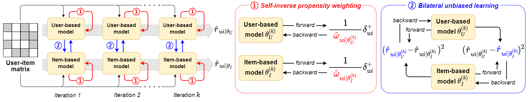
To eliminate exposure bias, we propose a novel unbiased recommender learning model, namely the BIlateral SElf-unbiased Recommender (BISER) with two key components: self-inverse propensity weighting (SIPW) and bilateral unbiased learning (BU). Motivated by self-distillation (Mobahi et al., 2020; Yang et al., 2019), we first devise a self-inverse propensity weighting (SIPW) to iteratively mitigate the exposure bias of items. Specifically, we reuse the model prediction from the previous training iteration, enabling us to gradually eliminate the exposure bias of items as the training evolves. Notably, SIPW has two key advantages: (i) it effectively handles the exposure bias caused by recommender models and (ii) it does not require an additional model for propensity score estimation.
IPW usually suffers from the high variance problem, as reported in the literature (Zhang et al., 2021; Wei et al., 2021). To resolve this issue, we first assume that the true user preference should be consistent with the predictions of different models. We then design bilateral unbiased learning (BU) using two recommender models. Specifically, we utilize user- and item-based autoencoders (Sedhain et al., 2015). Because they capture different hidden patterns on the user and item sides, it does not require us to split the training and estimation subsets from an entire training set (Zhu et al., 2020) or to utilize multiple models with different parameter initializations (Saito, 2020a). We exploit the predicted value of one model as a pseudo-label for another model. As a result, we resolve the high-variance issue in estimating the SIPW.
To summarize, the key contributions of this paper are as follows:
-
•
We review existing studies on unbiased recommender learning and analyze their limitations to eliminate the exposure bias of items caused by recommender models (Section 2).
-
•
We propose a novel unbiased recommender learning model, namely BIlateral SElf-unbiased Recommender (BISER), utilizing (i) a learning-based propensity score estimation method, i.e., self-inverse propensity weighting (SIPW), and (ii) bilateral unbiased learning (BU) using user- and item-based autoencoders with complementary relationships (Section 3).
-
•
We demonstrate that the BISER outperforms state-of-the-art unbiased recommender models, including RelMF (Saito et al., 2020), AT (Saito, 2020a), CJMF (Zhu et al., 2020), PD (Zhang et al., 2021), and MACR (Wei et al., 2021), on both unbiased evaluation datasets (e.g., Coat and Yahoo! R3) and conventional datasets (e.g., MovieLens and CiteULike) (Sections 4–5).
 |
|
| (a) MF | (b) Unbiased MF (ours) |
 |
|
| (c) AE | (d) Unbiased AE (ours) |
2. Background
Notations. Formally, we denote as a set of users and as a set of items. We are given a user-item click matrix ,
| (1) |
We model as a Bernoulli random variable, indicating the interaction of a user on an item . For implicit feedback data, the user interaction is a result of observation and preference. That is, a user may click on an item if (i) the item is exposed to the user and the user is aware of the item (exposure) and (ii) the user is actually interested in the item (relevance). Existing studies (Schnabel et al., 2016; Saito, 2020b; Saito et al., 2020; Chen et al., 2020; Zhu et al., 2020; Qin et al., 2020) formulate this idea as follows:
| (2) |
where is an element of the observation matrix that represents whether the user has observed the item () or not (), and is an element of the relevance matrix , representing true relevance regardless of observance. If the user likes the item , , and otherwise. For simplicity, we denote and with and , respectively. The interaction matrix Y with biased user behavior is decomposed into element-wise multiplication of the observation and relevance components.
Unbiased recommender learning. Our goal is to learn an unbiased ranking function from implicit feedback under the MNAR assumption. Although there are various loss functions for training recommender models, such as point-wise, pair-wise, and list-wise losses (Rendle, 2021), we use the point-wise loss function in this paper. Given a set of user-item pairs , the loss function for biased interaction data is
| (3) |
where is the prediction matrix for R, and and are the loss of user on item for positive and negative preference, respectively. Under the point-wise loss setting, we adopt either the cross-entropy or the sum-of-squared loss. With the cross-entropy, for example, and .
Similarly, the ideal loss function that relies purely on relevance is formulated as follows:
| (4) |
where the biased observation is substituted with the pure relevance .
Because user interaction data are typically sparse and collected under the MNAR assumption, it is necessary to bridge the gap between the loss functions for clicks and relevance. Saito et al. (2020) proposed a loss function using inverse propensity weighting (IPW):
| (5) |
where is the inverse propensity score that indicates the probability of observing the item by the user . As proved in (Saito et al., 2020), the expectation of the unbiased loss function in Eq. (5) is equivalent to the ideal loss function in Eq. (4):
| (6) |
The critical issue is how to estimate the propensity score from observed feedback (e.g., clicks). Previous studies (Saito et al., 2020; Saito, 2020b; Zhu et al., 2020; Qin et al., 2020; Lee et al., 2021) have developed several solutions to estimate . First, (Saito et al., 2020; Saito, 2020b; Lee et al., 2021) introduced a heuristic function to estimate item popularity without using an additional model. Although intuitive, it focuses only on addressing item popularity and is thus, incapable of handling exposure bias caused by recommender models. Second, additional models were used to estimate the propensity score (Zhu et al., 2020; Qin et al., 2020). However, this incurs high computational costs, as they mostly utilize three or more models.
3. BISER: Proposed Model
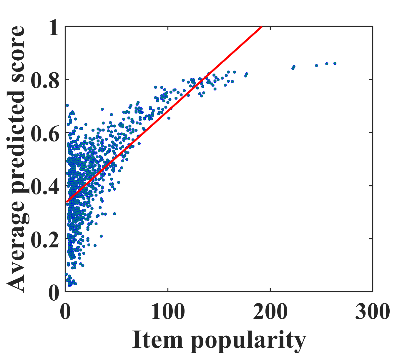
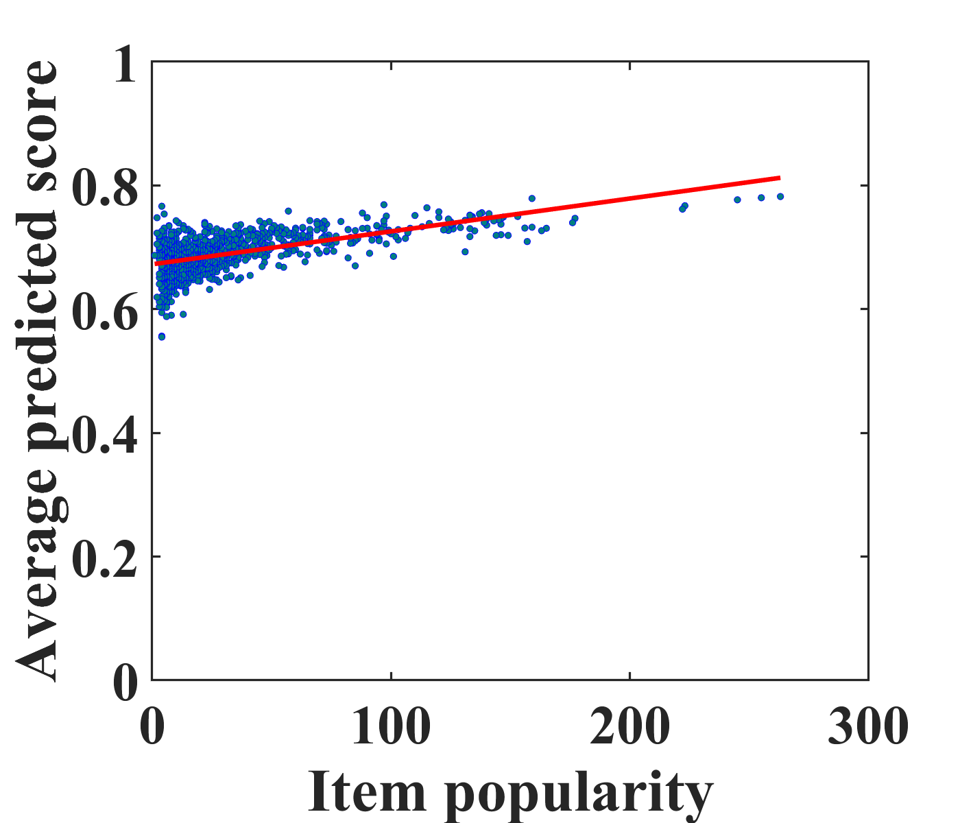
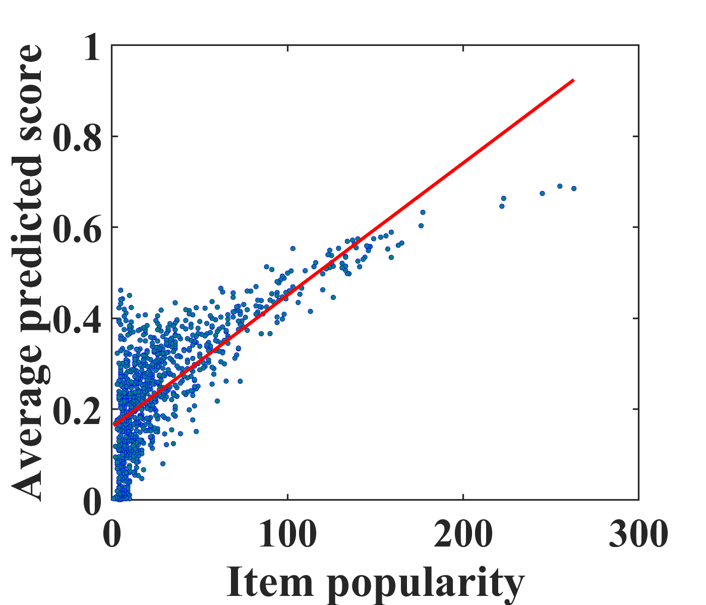
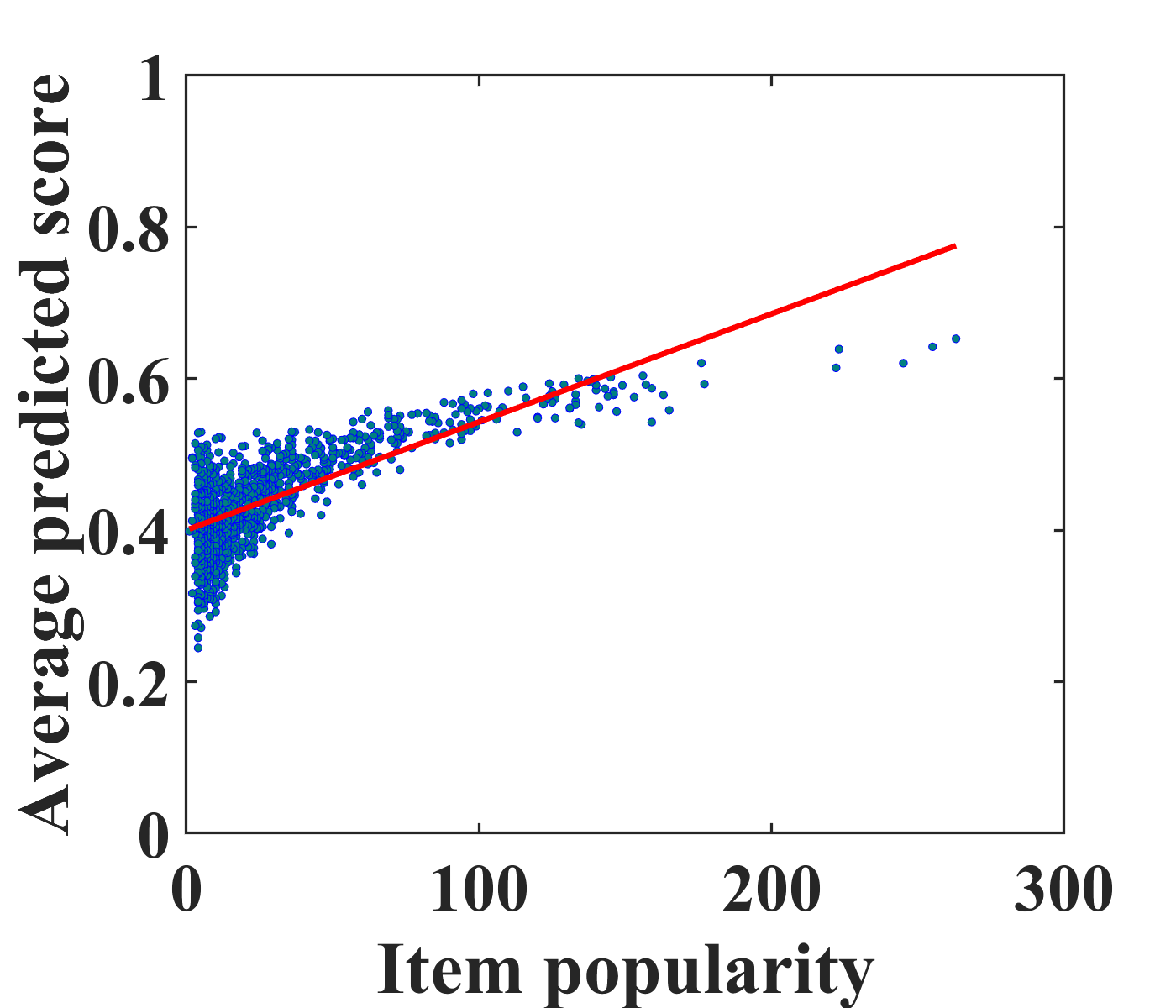
To motivate unbiased recommender modeling, we first investigate the bias from conventional recommendation models, i.e., matrix factorization (MF) and autoencoders (AE) (Sedhain et al., 2015) on the MovieLens-100K (ML-100K) dataset. Figures 2(a) and (c) depict a positive correlation between the average predicted scores for clicked items and the number of ratings in the training set, i.e., popularity. From this case study, we confirm that popular items tend to be recommended to more users with conventional models. Even worse, the biased recommendations can exacerbate the bias of the training dataset as user feedback is continually collected.
To address this problem, it is vital to eliminate the exposure bias caused by recommender models. Existing studies (Saito, 2020b; Saito et al., 2020) have mainly focused on modeling the popularity bias of items. Because user experiences are mostly biased towards the recommended items, we aim to eliminate exposure bias caused by recommender models. We estimate the propensity score of the items and eliminate exposure bias during model training. Figures 2(b) and (d) show the effectiveness of the proposed unbiased learning method. It is clearly observed that the correlation between the actual and predicted ratings in the proposed model is weaker than that in the traditional models. This pilot study indicates that our unbiased model effectively reduces exposure bias caused by recommender models.
3.1. Model Architecture
In this section, we present the novel unbiased recommender model, namely, the Bilateral Self-unbiased Recommender (BISER). Specifically, it consists of two parts: self-inverse propensity weighting (SIPW) and bilateral unbiased learning (BU), as shown in Figure 1. Motivated by self-distillation (Mobahi et al., 2020; Yang et al., 2019), which extracts knowledge of model predictions during model training, we estimate inverse propensity weighting (IPW) in an iterative manner. Thus, the proposed model gradually eliminates the exposure bias of items during model training. It is efficient because it neither requires a pre-defined propensity scoring function nor an additional model for propensity estimation.
In this process, we adopt two recommender models with complementary characteristics, user- and item-based autoencoders that capture heterogeneous semantics and relational information from the users’ and items’ perspectives, respectively. This bypasses the estimation overlap issue that occurs when the outputs of multiple models with the same structure and trained on the same training sets, converge similarly. Furthermore, we emphasize that our proposed approach is model-agnostic; two or more models may be used as long as they convey heterogeneous signals from the user-item interaction data.
Self-inverse propensity weighting (SIPW). Existing studies deal with eliminating the exposure bias in two ways: (i) by modeling only item popularity, which affects the clicking behavior of users, regardless of an additional estimator (Saito et al., 2020; Saito, 2020b), or (ii) by adopting an additional model to estimate the exposure bias by interleaving relevance and observation estimation (Zhu et al., 2020). Zhu et al. (2020) split an entire dataset into multiple training and estimation subsets, incurring high computational costs.
In this paper, we formulate a new bias estimation method, namely self-inverse propensity weighting (SIPW). First, we introduce an ideal unbiased recommender model using interaction data. Given a recommender list of items to user , the probability of the user interacting with an item is given by
| (7) |
where is the ideal probability of observing an item , i.e., completely-at-random distribution. Besides, we estimate the probability that the user interacts with the item by the biased recommender model as
| (8) |
where is the estimated probability of observing an item .
By combining them, we estimate the IPS as the ratio between the two probability distributions for interactions. Note that this formulation is closely related to the unbiased learning-to-rank method (Wang et al., 2016).
| (9) |
Assuming follows uniform distribution, the probability for every item in is simply regarded as a constant. Therefore, we estimate a propensity score as
| (10) |
The remaining issue is how to estimate the probability of observing item by user . Inspired by self-distillation (Mobahi et al., 2020; Yang et al., 2019) that utilizes the knowledge of model predictions during model training, we reuse the model prediction as . Despite its simplicity, self-propensity estimation has several benefits. (i) Our SIPW method stably estimates by regularizing prior knowledge, gradually removing the bias. (ii) It does not require an additional inference process to estimate the propensity scores. (iii) Owing to the model-agnostic property, our solution can be applied with various recommender models, e.g., MF (Hu et al., 2008) and AE (Sedhain et al., 2015).
Formally, we formulate an unbiased loss function using SIPW as
| (11) | ||||
where is the model parameter at the -th iteration and is the self-inverse propensity score at the -th iteration.
Bilateral unbiased learning (BU). Although IPW is theoretically principled, it often leads to suboptimal performance owing to the high variance problem in practice (Swaminathan and Joachims, 2015; Gilotte et al., 2018; Wang et al., 2019). An existing study (Saito, 2020a) trains multiple models where the prediction from one model is used as the pseudo-label for the other models. The pseudo-label is then used to regularize the original model. Although it helps mitigate the high-variance problem, multiple models can show a similar tendency as they are trained.
To resolve this issue, we utilize two recommender models with different characteristics. Unifying user- and item-based recommender models improves predictions in conventional recommender models (Wang et al., 2006; Yamashita et al., 2011; Zhu et al., 2019). As they tend to capture different aspects of user and item patterns, adopting heterogeneous models helps to relax the estimation overlap issue.
Specifically, we utilize user- and item-based autoencoders to discover unique and compensating patterns from complex user-item interactions. Inspired by label shift (Lipton et al., 2018; Azizzadenesheli et al., 2019), the two models should converge to the same value to correctly estimate the true relevance.
| (12) |
where and are the parameters of user- and item-based autoencoders, respectively (Sedhain et al., 2015). Finally, we present a loss function for bilateral unbiased learning using the two model predictions.
| (13) |
where and are predictions from each model at the -th iteration, respectively. is a set of observed user-item pairs.
3.2. Training and Inference
Given user- and item-based autoencoders, each model is trained from scratch using SIPW. At each iteration, we update the model parameters by minimizing the loss in Eq. (11). We then account for the loss function to minimize the difference between the two model predictions. Specifically, the user-based model with parameter is trained with the predictions from the item-based model with parameter as pseudo-labels, and vice versa. Therefore, we can reduce the high-variance issue of SIPW by using two model predictions.
Based on Eq. (11) and (13), we represent the final loss function to simultaneously train two models at the -th iteration.
| (14) |
| (15) |
where and are the hyperparameters to control the importance of .
Once model training is terminated, the biases of the two models are eliminated from the users’ and items’ perspectives. By unifying user preferences from different perspectives, we can improve model predictions (Wang et al., 2006; Yamashita et al., 2011; Zhu et al., 2019). Finally, we use the average of the predictions of the two models for the final rating.
| (16) |
The pseudo-code of BISER with user- and item-based AE is described in Algorithm 1. In the learning process, it first initializes the parameters and of both AE (line 1). Subsequently, and are updated using Eqs. (14) and (15) with the model predictions from the previous iteration, respectively (lines 2-5). At each iteration, it calculates the predictions of both models for all the clicked user-item pairs. After the two-model training is terminated, we obtain the predicted matrix using the two model predictions (lines 6 and 7).
4. Experimental Setup
Datasets and preprocessing. Table 1 summarizes the statistics of the datasets used in the evaluation. Among these datasets, the Coat and Yahoo! R3 datasets are specially designed to evaluate an unbiased setting. Specifically, their training set collected user feedback without special treatment (so it is likely to be biased), but the test set was carefully designed to be unbiased by explicitly asking for feedback for a pre-selected random set of items from each user. These two datasets are ideal for evaluating unbiased recommender models in a controlled setting. We also used four benchmark datasets, i.e., MovieLens (ML)-100K, ML-1M, ML-10M, and CiteULike, where the training and test datasets are inherently collected with click bias.
To account for implicit feedback, five datasets with explicit feedback (i.e., Coat111https://www.cs.cornell.edu/~schnabts/mnar/, Yahoo! R3222http://webscope.sandbox.yahoo.com/, MovieLens333http://grouplens.org/datasets/movielens/ (ML)-100K, ML-1M, and ML-10M) are converted into implicit feedback. We treat the items with four or higher scores as positive feedback and the remaining ratings are regarded as missing feedback. Unlike the other five datasets, CiteULike (Wang et al., 2015) provides implicit feedback.
We conduct the following experiments with different settings:
-
•
MNAR-MAR: Using Coat and Yahoo! R3, we train the model on the training dataset collected under the MNAR assumption and evaluate it on the test set collected under MAR. The training and test sets are provided separately. Within the training set, we set 30% of the ratings per user for validation purposes. The test set of the Coat and Yahoo! R3 datasets consists of 16 and 10 item ratings per user, respectively. For the items in the test set, we retrieve the top- items.
-
•
MNAR-MNAR: Using four traditional datasets, we train and evaluate the recommender models under the MNAR assumption. Before splitting the dataset, we removed users who rated 10 or fewer items and items rated by 5 or fewer users. For each user, we randomly held 80% and 20% as the training and test sets, respectively, and further split 30% of the training set into the validation set. Then, we evaluate the top- recommendation for all unrated items.
| Datasets | #users | #items | #interactions | Sparsity |
|---|---|---|---|---|
| Coat | 290 | 300 | 1,905 | 0.978 |
| Yahoo! R3 | 15,400 | 1,000 | 125,077 | 0.992 |
| ML-100K | 897 | 1,007 | 54,103 | 0.940 |
| ML-1M | 5,950 | 3,125 | 573,726 | 0.969 |
| ML-10M | 66,028 | 8,782 | 4,977,095 | 0.991 |
| CiteULike | 5,551 | 15,452 | 205,813 | 0.998 |
| NDCG | MAP | Recall | ||||||||
| Datasets | Models | = 1 | = 3 | = 5 | = 1 | = 3 | = 5 | = 1 | = 3 | = 5 |
| Coat | MF (Hu et al., 2008) | 0.3748 | 0.3441 | 0.3714 | 0.1346 | 0.2100 | 0.2566 | 0.1346 | 0.2592 | 0.3705 |
| UAE (Sedhain et al., 2015) | 0.3610 | 0.3546 | 0.3815 | 0.1265 | 0.2165 | 0.2648 | 0.1265 | 0.2785 | 0.3869 | |
| IAE (Sedhain et al., 2015) | 0.3655 | 0.3560 | 0.3812 | 0.1311 | 0.2185 | 0.2651 | 0.1311 | 0.2769 | 0.3847 | |
| RelMF (Saito et al., 2020) | 0.3959 | 0.3659 | 0.3922 | 0.1484 | 0.2281 | 0.2758 | 0.1484 | 0.2819 | 0.3926 | |
| AT (Saito, 2020a) | 0.4017 | 0.3652 | 0.3912 | 0.1517 | 0.2286 | 0.2753 | 0.1517 | 0.2772 | 0.3908 | |
| PD (Zhang et al., 2021) | 0.3997 | 0.3543 | 0.3737 | 0.1433 | 0.2182 | 0.2606 | 0.1433 | 0.2622 | 0.3627 | |
| MACR (Wei et al., 2021) | 0.4176 | 0.3798 | 0.3973 | 0.1559 | 0.2389 | 0.2834 | 0.1559 | 0.2875 | 0.3870 | |
| CJMF† (Zhu et al., 2020) | 0.4093 | 0.3856 | 0.4097 | 0.1500 | 0.2408 | 0.2900 | 0.1500 | 0.2984 | 0.4075 | |
| BISER (ours) | 0.4503∗ | 0.4109∗ | 0.4378∗∗ | 0.1725∗ | 0.2663∗∗ | 0.3192∗∗ | 0.1725∗ | 0.3185∗ | 0.4367∗∗ | |
| Gain (%) | 10.03 | 6.56 | 6.85 | 14.99 | 10.58 | 10.08 | 14.99 | 6.74 | 7.16 | |
| Yahoo! R3 | MF (Hu et al., 2008) | 0.1797 | 0.2081 | 0.2411 | 0.1071 | 0.1688 | 0.1970 | 0.1071 | 0.2225 | 0.3040 |
| UAE (Sedhain et al., 2015) | 0.1983 | 0.2235 | 0.2532 | 0.1198 | 0.1836 | 0.2104 | 0.1198 | 0.2362 | 0.3111 | |
| IAE (Sedhain et al., 2015) | 0.2137 | 0.2355 | 0.2653 | 0.1309 | 0.1956 | 0.2232 | 0.1309 | 0.2461 | 0.3211 | |
| RelMF (Saito et al., 2020) | 0.1837 | 0.2122 | 0.2453 | 0.1102 | 0.1728 | 0.2014 | 0.1102 | 0.2266 | 0.3080 | |
| AT (Saito, 2020a) | 0.1912 | 0.2179 | 0.2506 | 0.1149 | 0.1786 | 0.2071 | 0.1149 | 0.2310 | 0.3125 | |
| PD (Zhang et al., 2021) | 0.1994 | 0.2308 | 0.2647 | 0.1211 | 0.1901 | 0.2207 | 0.1211 | 0.2459 | 0.3297 | |
| MACR (Wei et al., 2021) | 0.2044 | 0.2274 | 0.2571 | 0.1243 | 0.1882 | 0.2154 | 0.1243 | 0.2382 | 0.3133 | |
| CJMF† (Zhu et al., 2020) | 0.2151 | 0.2426 | 0.2715 | 0.1320 | 0.2018 | 0.2291 | 0.1320 | 0.2564 | 0.3297 | |
| BISER (ours) | 0.2323∗∗ | 0.2608∗∗ | 0.2894∗∗ | 0.1446∗∗ | 0.2195∗∗ | 0.2479∗∗ | 0.1446∗∗ | 0.2748∗∗ | 0.3477∗∗ | |
| Gain (%) | 7.99 | 7.52 | 6.60 | 9.58 | 8.77 | 8.20 | 9.58 | 7.18 | 5.47 | |
| Datasets | Models | NDCG1 | NDCG3 | NDCG5 |
|---|---|---|---|---|
| Coat | MF | 0.3748 | 0.3441 | 0.3714 |
| + Rel-IPW | 0.3959 | 0.3659 | 0.3922 | |
| + Pre-SIPW | 0.4162 | 0.3867 | 0.4120 | |
| + SIPW | 0.3993 | 0.3686 | 0.3963 | |
| UAE | 0.3610 | 0.3546 | 0.3815 | |
| + Rel-IPW | 0.3876 | 0.3720 | 0.4031 | |
| + Pre-SIPW | 0.3990 | 0.3766 | 0.3982 | |
| + SIPW | 0.4262 | 0.3973 | 0.4259 | |
| IAE | 0.3655 | 0.3560 | 0.3812 | |
| + Rel-IPW | 0.3990 | 0.3716 | 0.3951 | |
| + Pre-SIPW | 0.4286 | 0.3939 | 0.4183 | |
| + SIPW | 0.4334 | 0.3949 | 0.4172 | |
| Yahoo! R3 | MF | 0.1797 | 0.2081 | 0.2411 |
| + Rel-IPW | 0.1837 | 0.2122 | 0.2453 | |
| + Pre-SIPW | 0.1870 | 0.2104 | 0.2405 | |
| + SIPW | 0.1881 | 0.2176 | 0.2496 | |
| UAE | 0.1983 | 0.2235 | 0.2532 | |
| + Rel-IPW | 0.2054 | 0.2384 | 0.2715 | |
| + Pre-SIPW | 0.2013 | 0.2256 | 0.2529 | |
| + SIPW | 0.2115 | 0.2461 | 0.2785 | |
| IAE | 0.2137 | 0.2355 | 0.2653 | |
| + Rel-IPW | 0.2146 | 0.2398 | 0.2708 | |
| + Pre-SIPW | 0.2120 | 0.2360 | 0.2645 | |
| + SIPW | 0.2190 | 0.2504 | 0.2802 |
Competing models. We compare BISER with three conventional recommender models, i.e., MF (Hu et al., 2008), UAE (Sedhain et al., 2015), and IAE (Sedhain et al., 2015), and five unbiased recommender models, i.e., RelMF (Saito et al., 2020), AT (Saito, 2020a), CJMF (Zhu et al., 2020), PD (Zhang et al., 2021), and MACR (Wei et al., 2021). Note that several methods (Saito et al., 2020; Saito, 2020a; Zhu et al., 2020; Zhang et al., 2021; Wei et al., 2021; Chen et al., 2021; Bonner and Vasile, 2018; Zheng et al., 2021) have been proposed to remove the bias in implicit feedback, but some methods (e.g., (Chen et al., 2021; Bonner and Vasile, 2018; Zheng et al., 2021)) require MAR training data; therefore, they are not included.
-
•
Matrix Factorization (MF) (Hu et al., 2008): The most popular recommender model for using linear factor embeddings in which the user preference score is predicted by a product of user- and item-embedding matrices.
-
•
User-based AutoEncoder (UAE) (Sedhain et al., 2015): This model learns non-linear item-item correlations for the users with a set of items using autoencoders.
-
•
Item-based AutoEncoder (IAE) (Sedhain et al., 2015): By transposing the rating matrix, this model learns non-linear user-user correlations, using autoencoders.
-
•
Relevance Matrix Factorization (RelMF) (Saito et al., 2020): This utilizes the MNAR scenario for model training, effectively removing the bias caused by item popularity. The IPW-based model estimates the propensity scores using a heuristic function for item popularity.
- •
-
•
Combinational Joint Learning for Matrix Factorization (CJMF) (Zhu et al., 2020): As an IPW-based model, it introduces a joint training framework to estimate both unbiased relevance and unbiased propensity using multiple sub-models. For our datasets, we set the number of sub-models to eight. It is one of the most compelling competitors due to the performance advantage of unbiased recommender learning.
- •
-
•
Model-Agnostic Counterfactual Reasoning (MACR) (Wei et al., 2021): This utilizes a cause-effect view by considering the direct effect of item properties on rank scores to remove the popularity bias. We report MACR using LightGCN (He et al., 2020) because LightGCN is better than BPRMF (Rendle et al., 2009).
Evaluation metrics. For top-N recommendation evaluation, we use three popular metrics: Normalized Discounted Cumulative Gain (NDCG@), Mean Average Precision (MAP@), and Recall@. We focus on measuring all metrics for the highest ranked items because predicting high-ranked items is critical. Considering the number of available ratings in the test set, we use for Coat and Yahoo! R3 datasets, while for ML-100K, ML-1M, ML-10M, and CiteULike datasets.
For MAR evaluation (Coat and Yahoo! R3), we adopt the Average-Over-All (AOA) evaluation, which is the conventional metric that evenly normalizes the scores for all items. For the MNAR evaluation (MovieLens and CiteULike), we use both AOA and unbiased evaluations. Yang et al. (2018) recently suggested an unbiased evaluation scheme and applies bias normalization to test scores. We follow the unbiased evaluation (Yang et al., 2018) and use for the normalization parameter.
We employ AOA and unbiased evaluation metrics in (Yang et al., 2018):
| (17) |
| (18) |
where denotes a set of clicked item to user in the test set and denotes the predicted ranking of item to user . Also, the function denotes any top-N scoring metrics (i.e., NDCG, MAP, and Recall), and the propensity is calculated by the popularity of the item . Because MNAR-MNAR evaluation does not have the ground-truth for unbiased test sets, it is difficult to measure the unbiased evaluation in eliminating the exposure bias of items. As an alternative, we evaluate whether the popularity bias is effectively eliminated, as done in (Yang et al., 2018), which is a more favorable setting for existing studies (Saito et al., 2020; Saito, 2020a) that handle item popularity bias.
Reproducibility. For all models, trainable weights are initialized using Xavier’s method (Glorot and Bengio, 2010). Except for PD (Zhang et al., 2021) and MACR (Wei et al., 2021), we optimized using Adagrad (Duchi et al., 2010), and for PD (Zhang et al., 2021) and MACR (Wei et al., 2021), we optimized using Adam (Kingma and Ba, 2015). For the MF-based models, the batch size is set to 1,024 () for Coat, Yahoo! R3, and MovieLens, and 16,384 () for CiteULike. Meanwhile, for the LightGCN-based model, the batch size is set to 2,048 and 8,192 for Coat and the remaining datasets, respectively. For the AE-based models, the batch size is set to one user/item by default. We performed a grid search to tune the latent dimension over {50, 100, 200, 400} for the AE-based models and {32, 64, 128, 256} for the MF- and LightGCN-based models. We also searched for the learning rate within [2e-1, 1e-5] and L2-regularization within the range of [1e-4, 1e-14] for each model. For the proposed BISER, we tuned two coefficients, and , between {0.1, 0.5, 0.9}. Additionally, we set the maximum training epoch to 500. We also perform early stopping with five patience epochs for NDCG and NDCG in the MNAR-MAR and MNAR-MNAR settings, respectively. To implement RelMF (Saito et al., 2020), CJMF (Zhu et al., 2020), PD (Zhang et al., 2021), and MACR (Wei et al., 2021), we used the codes provided by each author. Our code and detailed hyperparameter settings are available at https://github.com/Jaewoong-Lee/sigir_2022_BISER.
5. Experimental results
In this section, we report extensive experimental results for BISER in both the MNAR-MAR and MNAR-MNAR settings. We also analyze the performance of BISER by item group and the effectiveness of each component (i.e., SIPW and BU) in the MNAR-MAR setting. For the MNAR-MAR setting, we reasonably validate the effectiveness of BISER. For the MNAR-MNAR setting, we also evaluate whether BISER is still effective in general evaluation environments.
5.1. MNAR-MAR Evaluation
Performance comparison. Table 2 reports the comparison results between BISER and the other competing models. From these results, we obtained several intriguing findings. First, BISER demonstrates significant and consistent performance gains across all metrics by 6.56-14.99% on Coat and 5.47-9.58% on Yahoo! R3, achieving state-of-the-art performance. This indicates that BISER is more effective in eliminating the bias than existing unbiased models because the high performance on MAR test sets indicates that the bias is successfully removed, or at least, our proposed model is more robust to bias than the competing models. Second, the unbiased models (RelMF, AT, PD, MACR, CJMF, and BISER) generally outperform the traditional models (UAE, IAE, and MF). This potentially implies that eliminating bias in the click data can improve the user experience. Finally, among the existing unbiased models, CJMF achieves better accuracy than other MF-based models due to an ensemble effect from eight sub-models and MACR (Wei et al., 2021) also shows competitive performance among the existing models.
 |
 |
 |
| (a) Coat | ||
 |
 |
 |
| (b) Yahoo! R3 | ||
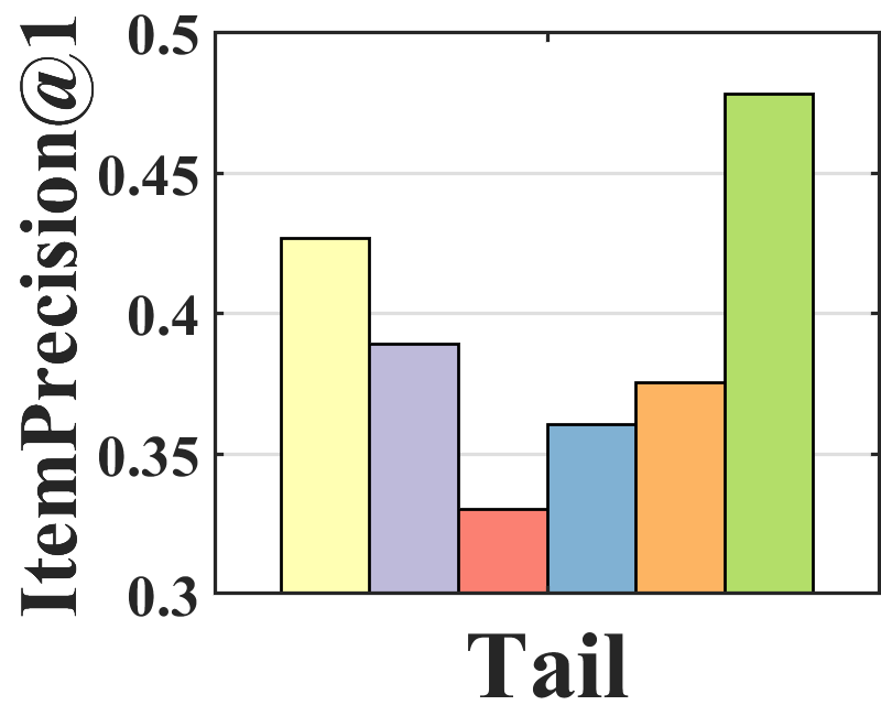
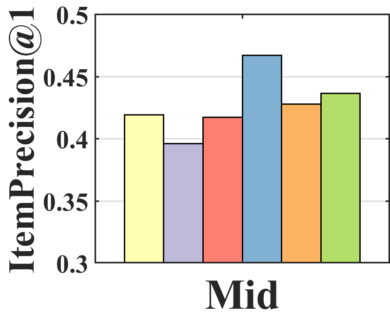
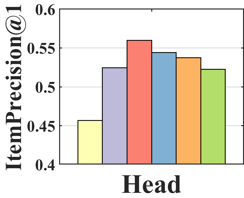
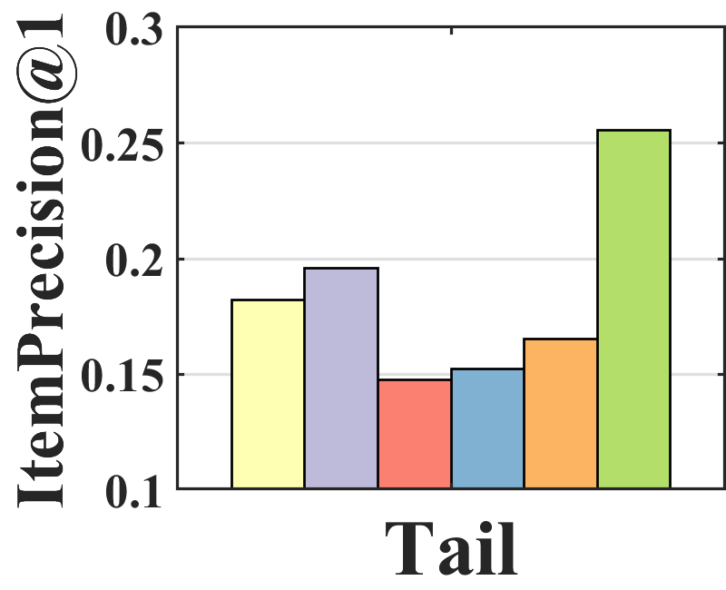
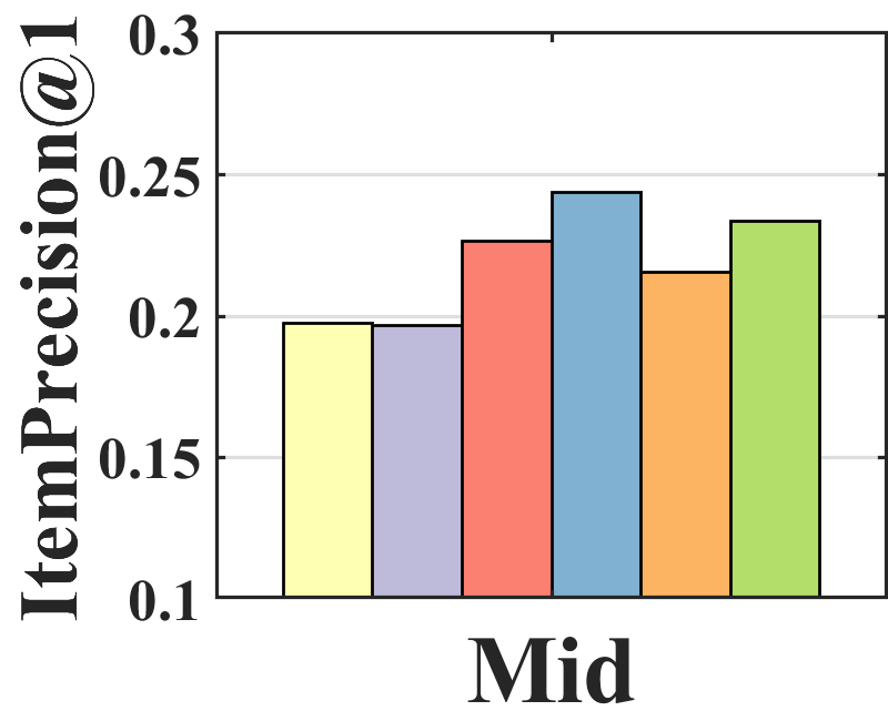
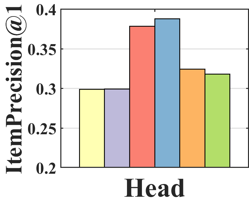
Performance analysis. To analyze where the performance improvement of BISER comes from, we investigate the performance of each item group according to item popularity. Specifically, we sort all items based on their popularity and split them into three groups (i.e., tail, mid, and head) with an equal number of interactions. Figure 3 shows the average of ItemPrecision1 for each item group. ItemPrecisionN refers to the ratio of the items that appear in the relevance set to the top-N items for all users.
| (19) |
As depicted in Figure 3, each model shows a different performance trend in the item groups. BISER shows a significantly higher performance than the baselines in the tail group. This means that BISER correctly predicts at user’s preference for unpopular items. RelMF (Saito et al., 2020) and AT (Saito, 2020a) show similar performance over the three groups, whereas PD (Zhang et al., 2021) and MACR (Wei et al., 2021) show relatively high performance in the mid and head groups. This indicates that the performance gains of PD (Zhang et al., 2021) and MACR (Wei et al., 2021) mainly come from the popular item group. That is, BISER removes bias more effectively than other competing models, including the causal graph-based method. In addition, the higher the popularity (i.e., tail mid head), the higher is the overall performance of all the baselines. This shows that all the models more easily predict users’ preferences for popular items than for unpopular items because popular items tend to be biased in training recommender models.
Effect of self-inverse propensity weighting (SIPW). To validate the effectiveness of SIPW, we compare four different groups of models: (i) naïve models (i.e., MF, UAE, and IAE); (ii) models adopting the IPW module from Saito et al. (2020) (i.e., MF, UAE, and IAE + Rel-IPW); (iii) models with the pre-defined propensity as a prediction of the pre-trained model with biased click data (i.e., MF, UAE, and IAE + Pre-SIPW; a simple variant of SIPW); and (iv) models with SIPW (i.e., MF, UAE, and IAE + SIPW). Because of its model-agnostic properties, our poposed SIPW method can be applied to both MF- and AE-based models.
Table 3 shows that the SIPW outperforms Rel-IPW by up to 9.96% in Coat and up to 4.44% in Yahoo! R3 over NDCG1, 3, and 5. This suggests that SIPW helps eliminate the bias regardless of the backbone models. Additionally, the proposed method shows similar performance compared to pre-SIPW. This means that our approach of gradually removing bias without pre-training is efficient and effective in removing bias. In particular, the AE-based models have higher performance improvements than MF-based models. Because the AE-based models represent non-linearity by their modeling power, we can further enjoy high-performance gains.
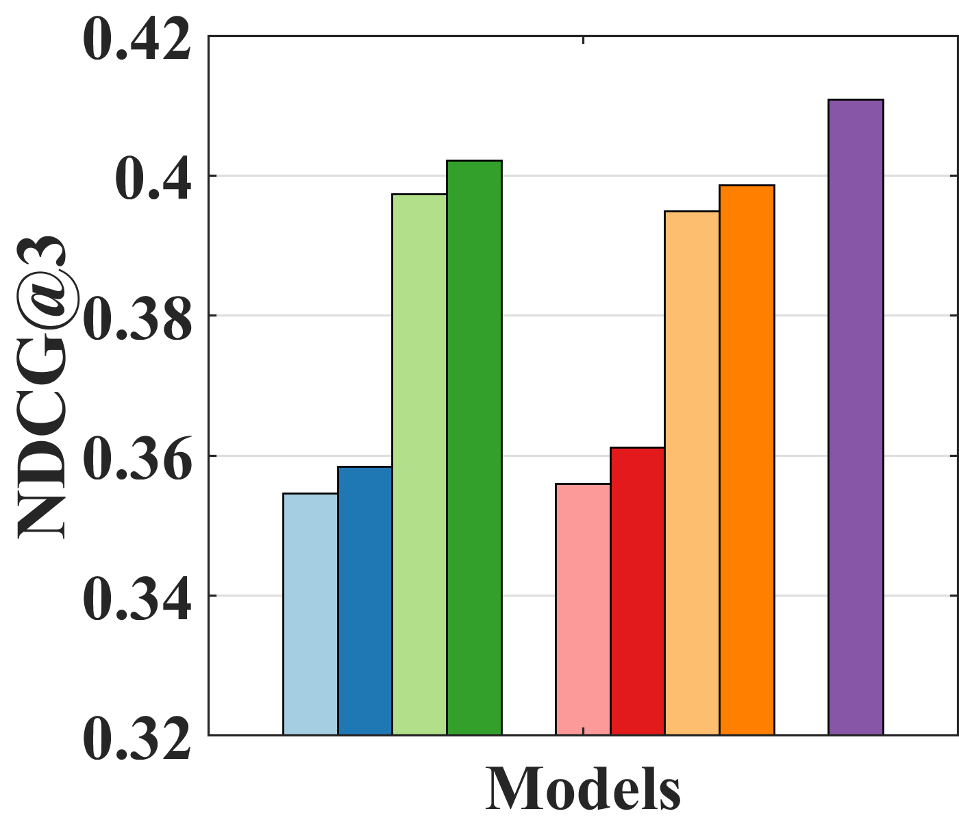
Effect of bilateral unbiased learning (BU). We design four different baselines: (i) AE-based naïve models (UAE and IAE); (ii) models with BU (UAE and IAE + BU); (iii) models with SIPW (UAE and IAE + SIPW); and (iv) models with both SIPW and BU (UAE and IAE + SIPW + BU). Figure 4 indicates that adopting BU in all models, except for IAE on Yahoo! R3, improves performance. Specifically, IAE + SIPW + BU is improved by 4.11% over IAE + SIPW on Coat and UAE + SIPW + BU over UAE + SIPW by 3.48% on Yahoo! R3 in terms of NDCG3. Although IAE slightly outperforms IAE + BU in Figure 4(b), IAE + SIPW + BU outperforms IAE + SIPW on Yahoo! R3 by 2.61% in terms of NDCG3. Because BU is adopted in the naïve models without removing bias, the bias of IAE + BU could be intensified, which might worsen the performance.
|
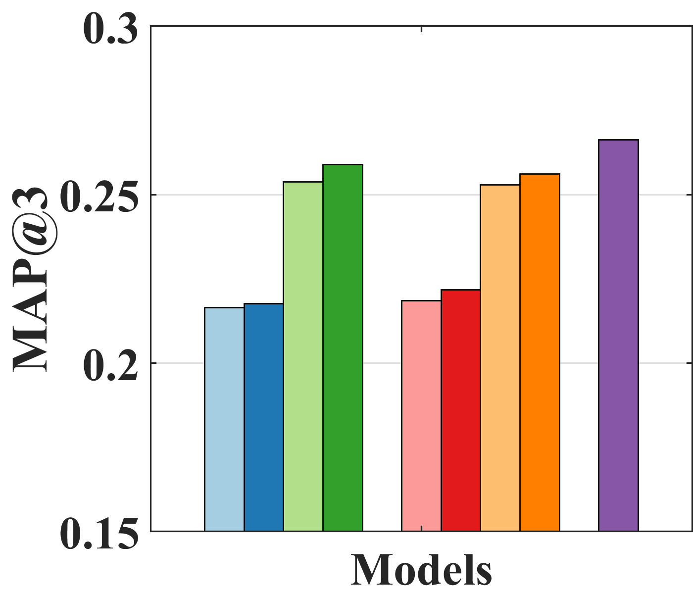 |
| (a) Coat | |
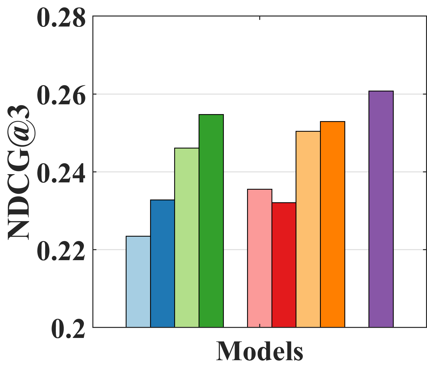 |
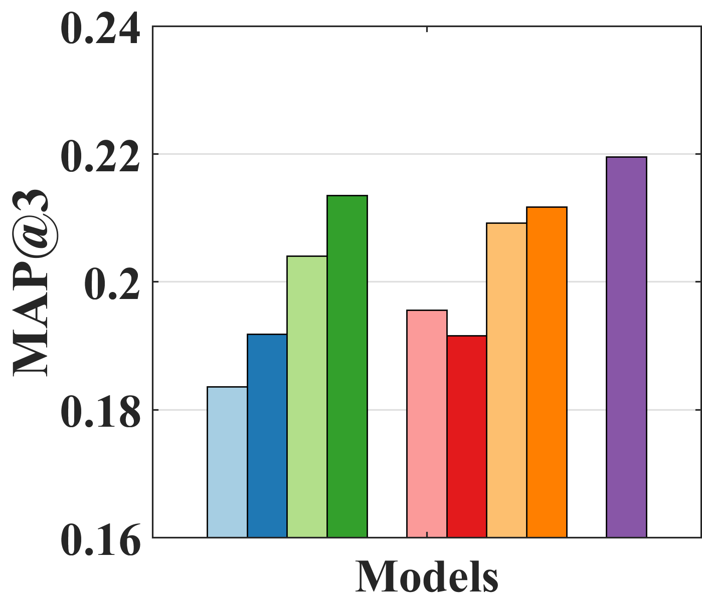 |
| (b) Yahoo! R3 | |
|
 |
| (a) Coat | (b) Yahoo! R3 |
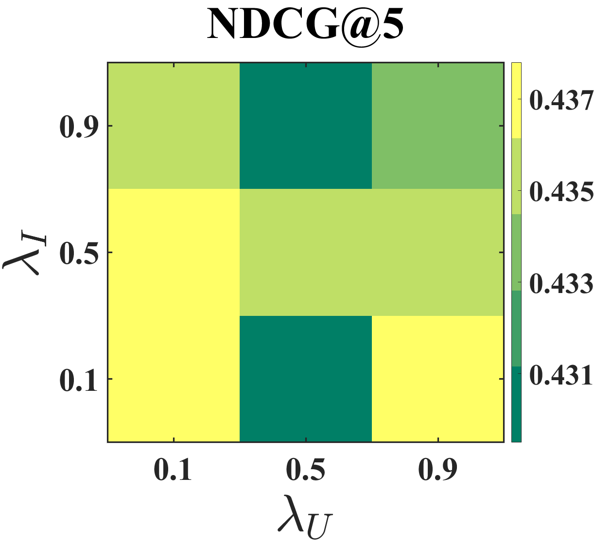
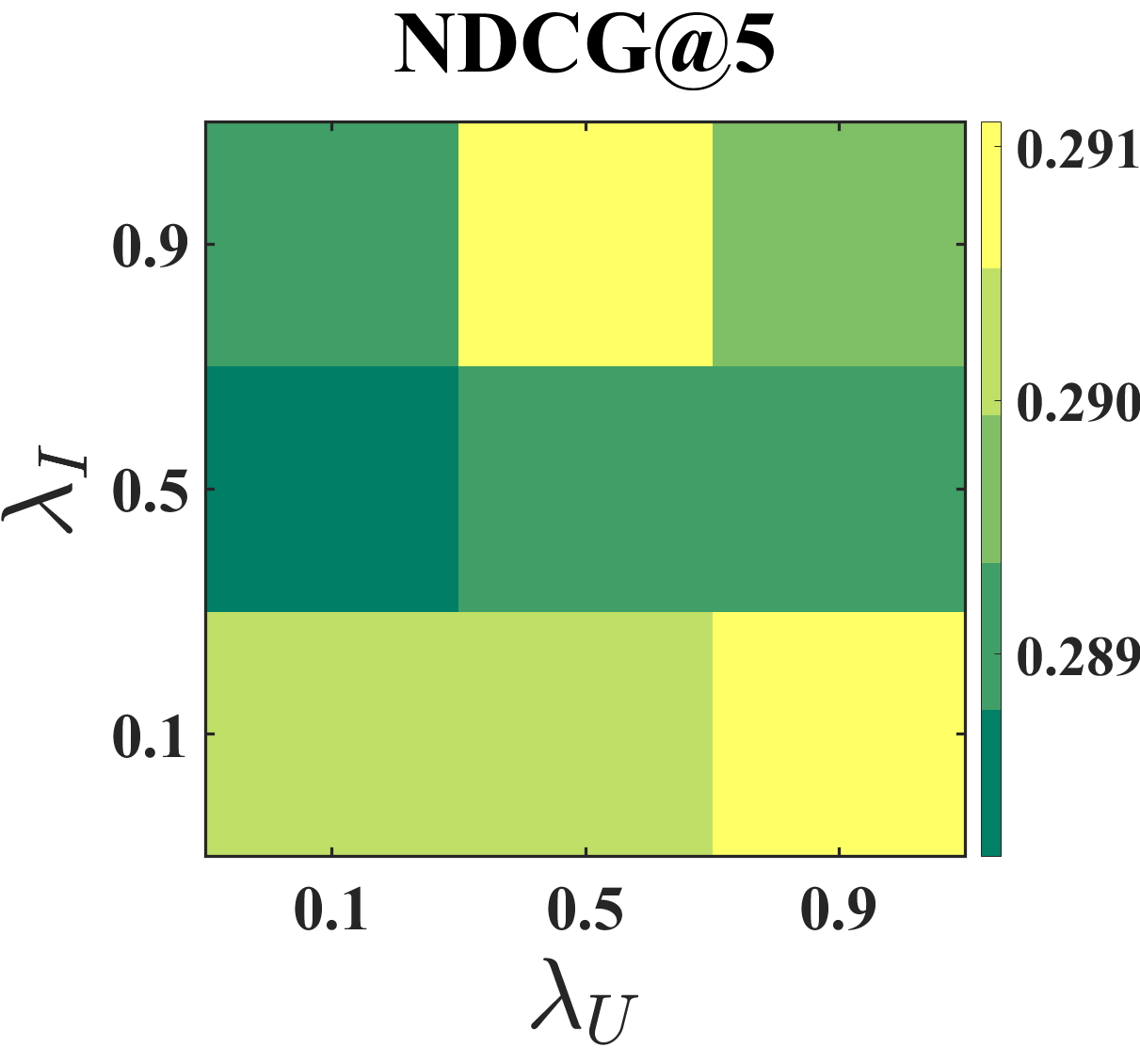
Effect of coefficients and . Figure 5 shows the result of the grid search on Coat and Yahoo! R3 datasets with two coefficients and in the range {0.1, 0.5, 0.9}. Specifically, the NDCG scores of BISER are between 0.4331–0.4378 in the Coat and 0.2890–0.2911 in the Yahoo! R3. For Coat, the proposed model tends to show high performances when and are relatively small values. For Yahoo! R3, our model tends to have high performance when and are large and small, respectively. Based on the performance trends, we set in Coat, and in Yahoo! R3. These results support the notion that the effects of SIPW and BU can vary depending on datasets.
|
 |
 |
 |
| (a) ML-100K | (b) ML-1M | (c) ML-10M | (d) CiteULike |
|
 |
 |
 |
| (a) ML-100K | (b) ML-1M | (c) ML-10M | (d) CiteULike |
5.2. MNAR-MNAR Evaluation
Performance comparison with unbiased evaluation. In the MNAR-MNAR setting, the test set is biased. We use the unbiased evaluation proposed by Yang et al. (2018) to measure the debiasing effect on the biased test set.
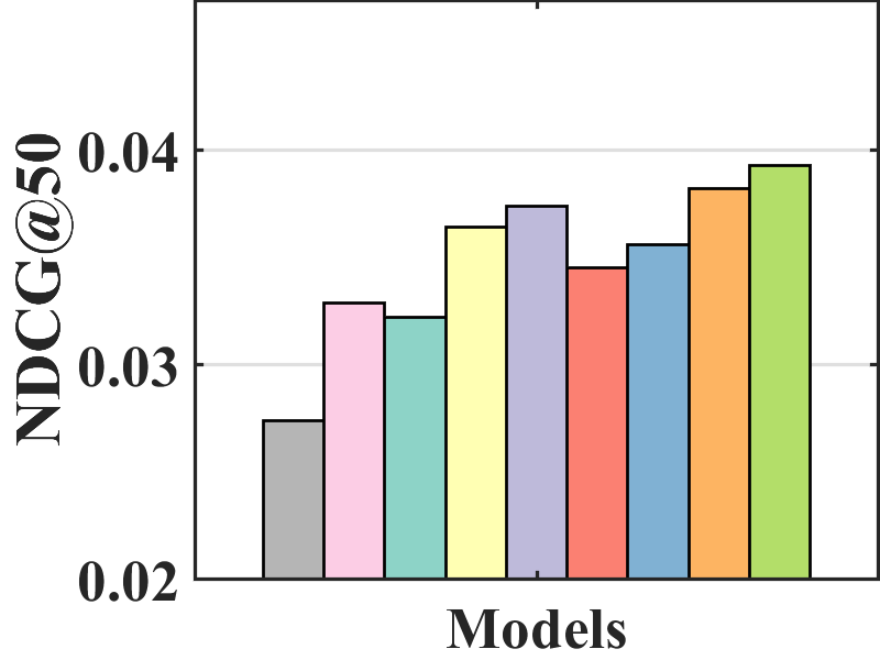
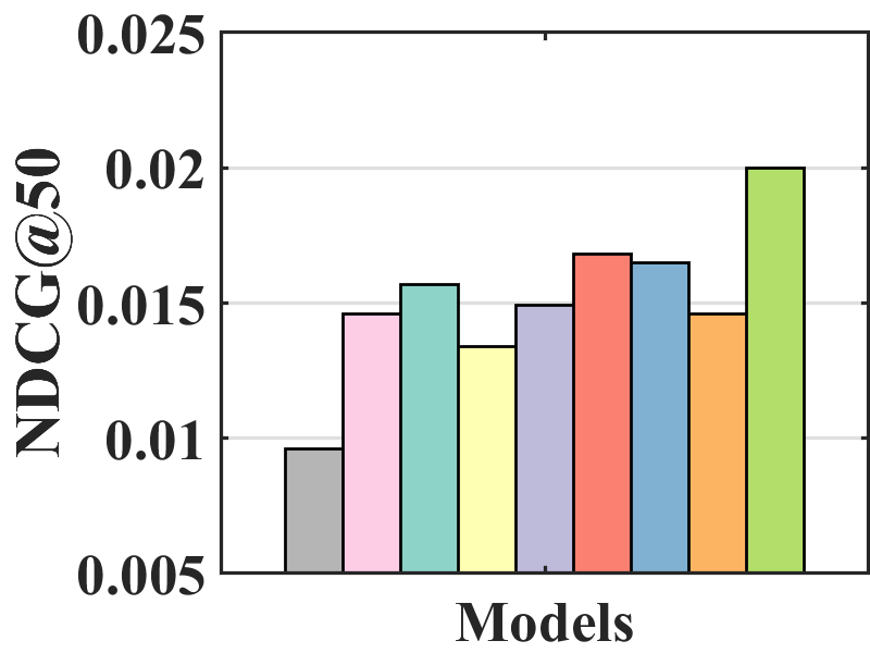
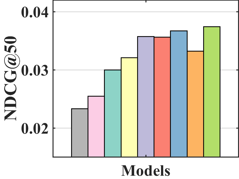
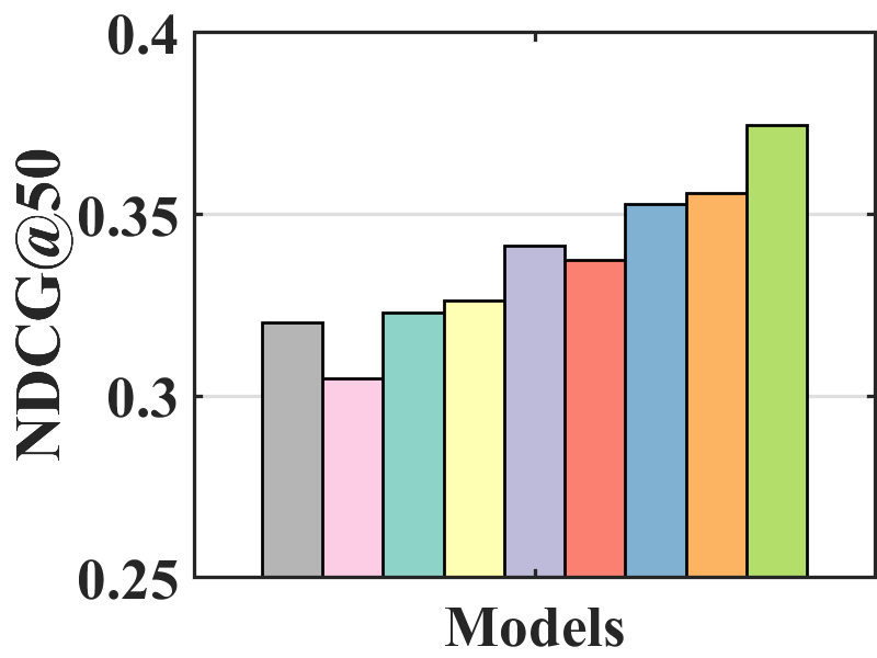
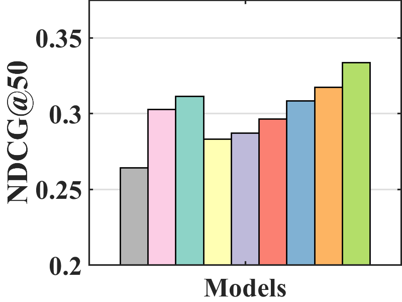
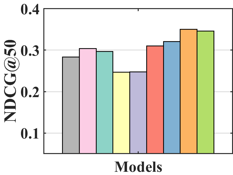
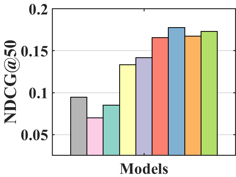
Figure 7 compares the performance of BISER with the baselines. We observe that BISER clearly and consistently outperforms the existing models. Specifically, BISER improved by 2.29, 19.32, 7.67, and 1.98% over the second-best models (i.e., CJMF, PD, PD, and MACR) in ML-100K, ML-1M, ML-10M, and CiteULike, respectively, in terms of NDCG50. This means that BISER effectively removes item bias regardless of data size and data type. Among the baselines, PD (Zhang et al., 2021) and MACR (Wei et al., 2021), using causal graphs, generally exhibit higher performance than IPW-based methods (i.e., RelMF (Saito et al., 2020) and CJMF (Zhu et al., 2020)). This indicates that PD (Zhang et al., 2021) and MACR (Wei et al., 2021) eliminate popularity bias.
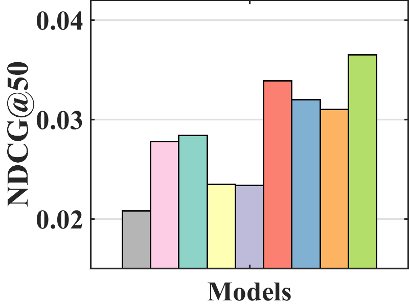
Performance comparison with AOA evaluation. In the MNAR-MNAR setting, AOA evaluation is the conventional evaluation protocol. As depicted in Figure 7, even in biased validation settings, BISER achieved a competitive performance over the other methods. Specifically, BISER performs best on the ML-100K and ML-1M datasets. In the ML-10M and CiteULike datasets, BISER shows the second-best model with a marginal difference from the best model. We conjecture that the success of BISER in MNAR-MNAR settings is possible by leveraging heterogeneous semantics using user- and item-based autoencoders via ensemble effects.
6. Related Work
Unbiased learning has been widely proposed for causal inference (Wang et al., 2016; Joachims et al., 2017; Wang et al., 2018a; Ai et al., 2018; Hu et al., 2019; Lee et al., 2020; Wang et al., 2021a; Ovaisi et al., 2020; Schnabel et al., 2016; Wang et al., 2021b, 2019; Saito, 2020a; Saito et al., 2020; Saito, 2020b; Zhu et al., 2020; Qin et al., 2020; Bonner and Vasile, 2018; Zhang et al., 2021; Wei et al., 2021; Zheng et al., 2021; Jeon et al., 2022) and missing data analyses (Marlin et al., 2007; Steck, 2010; Hernández-Lobato et al., 2014; Marlin and Zemel, 2009; Wang et al., 2018b; Ma and Chen, 2019; Liang et al., 2016). It has since been adopted to bridge the gap between interaction and relevance data in the information retrieval (IR) community, that is, unbiased learning-to-rank (LTR). Unbiased recommender learning, inspired by unbiased LTR, has been actively studied to eliminate bias from explicit and implicit feedback.
Unbiased learning with explicit feedback. Although explicit feedback provides both positive and negative samples, it is based on the MNAR assumption. To address this problem, existing studies are categorized into three types: imputation-based, IPW-based, and meta-learning-based methods. First, imputation-based methods (Marlin et al., 2007; Steck, 2010; Hernández-Lobato et al., 2014; Marlin and Zemel, 2009; Wang et al., 2018b; Ma and Chen, 2019) estimate missing ratings to reduce the biased statistics of user ratings. Steck (2010) imputed a predefined constant value to all missing ratings. Some studies utilized various recommender models to impute different ratings: Hernández-Lobato et al. (2014) and Wang et al. (2018b) used an MF model; Marlin et al. (2007) used a multinomial mixture model, and Marlin and Zemel (2009) used a conditional Bernoulli model. Ma and Chen (2019) adopted nuclear-norm-constrained matrix completion algorithm (Davenport et al., 2012) for rating imputation. Second, IPW-based methods (Schnabel et al., 2016; Wang et al., 2021b, 2019) estimate propensity scores for user-item ratings. Schnabel et al. (2016) first adopted the IPW method and predicted the propensity score using Naive Bayes or logistic regression. Wang et al. (2021b) trained a propensity estimator with few unbiased ratings. In addition, Wang et al. (2019) combined IPW and imputation methods to eliminate bias and take advantage of both methods. Recently, a meta-learning-based method (Saito, 2020a) was adopted to overcome the high-variance problem of IPW. Saito (2020a) trained a model using the output of one of multiple models as unbiased pseudo-labels.
Unbiased learning with implicit feedback. Unlike explicit feedback, implicit feedback provides only observed feedback. It is crucial to design an exposure bias for these items. Specifically, exposure bias can be considered for both user- and model-oriented reasons. Because users tend to recognize popular items, user clicks are biased towards popular items, i.e., popularity bias. To eliminate the popularity bias, Liang et al. (2016) determined the weight based on the prior probability of exposure. In addition, (Saito et al., 2020; Saito, 2020b; Zhu et al., 2020; Qin et al., 2020; Lee et al., 2021) used an IPW-based method to remove bias. While (Saito et al., 2020; Saito, 2020b) simply utilized the number of ratings per item (i.e., item popularity) as the propensity score, Zhu et al. (2020) used an additional model to estimate the propensity score. Qin et al. (2020) also introduced a propensity estimator that utilized additional attributes related to the recommender model (e.g., user interface of the application and type of recommender model). Lee et al. (2021) introduced a propensity score to both unclicked and clicked user feedback. Chen et al. (2021) used small unbiased feedback to eliminate bias. Additionally, causal embedding- and graph-based training methods (Bonner and Vasile, 2018; Zheng et al., 2021; Wei et al., 2021; Zhang et al., 2021) have been introduced to overcome the sensitivity of IPW strategies. Bonner and Vasile (2018) introduced causal embedding using small uniformly collected feedback. Zheng et al. (2021) introduced causal embedding and causal graph to disentangle user interests and conformity with small unbiased feedback. Wei et al. (2021) designed a causal graph with the item and user priors and Zhang et al. (2021) used causal intervention using a causal graph to eliminate bias. In contrast, our proposed method eliminates exposure bias caused by recommender models without additional assumptions for causality and model training.
7. Conclusion
This paper proposes a novel unbiased recommender model, namely BIlateral SElf-unbiased Recommender learning (BISER). To the best of our knowledge, this is the first paper to introduce self-inverse propensity weighting to eliminate exposure bias of items during model training. Then, we employed bilateral learning that takes advantage of user- and item-based autoencoders with heterogeneous information, capturing different hidden correlations across users/items. This process helped alleviate high variance in the estimated inverse propensity scores. Extensive experiments demonstrated that the BISER consistently outperformed existing unbiased recommender models in two evaluation protocols: MNAR-MAR and MNAR-MNAR settings.
References
- (1)
- Adomavicius and Tuzhilin (2005) Gediminas Adomavicius and Alexander Tuzhilin. 2005. Toward the Next Generation of Recommender Systems: A Survey of the State-of-the-Art and Possible Extensions. IEEE Trans. Knowl. Data Eng. 17, 6 (2005), 734–749.
- Ai et al. (2018) Qingyao Ai, Keping Bi, Cheng Luo, Jiafeng Guo, and W. Bruce Croft. 2018. Unbiased Learning to Rank with Unbiased Propensity Estimation. In SIGIR. 385–394.
- Azizzadenesheli et al. (2019) Kamyar Azizzadenesheli, Anqi Liu, Fanny Yang, and Animashree Anandkumar. 2019. Regularized Learning for Domain Adaptation under Label Shifts. In ICLR (Poster). OpenReview.net.
- Bonner and Vasile (2018) Stephen Bonner and Flavian Vasile. 2018. Causal embeddings for recommendation. In RecSys. ACM, 104–112.
- Chen et al. (2021) Jiawei Chen, Hande Dong, Yang Qiu, Xiangnan He, Xin Xin, Liang Chen, Guli Lin, and Keping Yang. 2021. AutoDebias: Learning to Debias for Recommendation. In SIGIR. 21–30.
- Chen et al. (2020) Jiawei Chen, Hande Dong, Xiang Wang, Fuli Feng, Meng Wang, and Xiangnan He. 2020. Bias and Debias in Recommender System: A Survey and Future Directions. CoRR abs/2010.03240 (2020).
- Choi et al. (2021) Minjin Choi, Yoonki Jeong, Joonseok Lee, and Jongwuk Lee. 2021. Local Collaborative Autoencoders. In WSDM. 734–742.
- Choi et al. (2022) Minjin Choi, Jinhong Kim, Joonsek Lee, Hyunjung Shim, and Jongwuk Lee. 2022. S-Walk: Accurate and Scalable Session-based Recommendationwith Random Walks. In WSDM.
- Davenport et al. (2012) Mark A. Davenport, Yaniv Plan, Ewout van den Berg, and Mary Wootters. 2012. 1-Bit Matrix Completion. CoRR abs/1209.3672 (2012).
- Duchi et al. (2010) John C. Duchi, Elad Hazan, and Yoram Singer. 2010. Adaptive Subgradient Methods for Online Learning and Stochastic Optimization. In COLT. 257–269.
- Gilotte et al. (2018) Alexandre Gilotte, Clément Calauzènes, Thomas Nedelec, Alexandre Abraham, and Simon Dollé. 2018. Offline A/B Testing for Recommender Systems. In WSDM. 198–206.
- Glorot and Bengio (2010) Xavier Glorot and Yoshua Bengio. 2010. Understanding the difficulty of training deep feedforward neural networks. In AISTATS, Vol. 9. 249–256.
- He et al. (2020) Xiangnan He, Kuan Deng, Xiang Wang, Yan Li, Yong-Dong Zhang, and Meng Wang. 2020. LightGCN: Simplifying and Powering Graph Convolution Network for Recommendation. In SIGIR. 639–648.
- He et al. (2018) Xiangnan He, Xiaoyu Du, Xiang Wang, Feng Tian, Jinhui Tang, and Tat-Seng Chua. 2018. Outer Product-based Neural Collaborative Filtering. In IJCAI. 2227–2233.
- He et al. (2017) Xiangnan He, Lizi Liao, Hanwang Zhang, Liqiang Nie, Xia Hu, and Tat-Seng Chua. 2017. Neural Collaborative Filtering. In WWW. 173–182.
- Hernández-Lobato et al. (2014) J.M. Hernández-Lobato, Neil Houlsby, and Z. Ghahramani. 2014. Probabilistic Matrix Factorization with Non-Random Missing Data. In ICML. II–1512–II–1520.
- Hu et al. (2008) Yifan Hu, Yehuda Koren, and Chris Volinsky. 2008. Collaborative Filtering for Implicit Feedback Datasets. In ICDM. 263–272.
- Hu et al. (2019) Ziniu Hu, Yang Wang, Qu Peng, and Hang Li. 2019. Unbiased LambdaMART: An Unbiased Pairwise Learning-to-Rank Algorithm. In WWW. 2830–2836.
- Jeon et al. (2022) Myeongho Jeon, Daekyung Kim, Woochul Lee, Myungjoo Kang, and Joonseok Lee. 2022. A Conservative Approach for Unbiased Learning on Unknown Biases. In CVPR.
- Joachims et al. (2017) Thorsten Joachims, Adith Swaminathan, and Tobias Schnabel. 2017. Unbiased Learning-to-Rank with Biased Feedback. In WSDM. 781–789.
- Kingma and Ba (2015) Diederik P. Kingma and Jimmy Ba. 2015. Adam: A Method for Stochastic Optimization. In ICLR.
- Lee et al. (2013) Joonseok Lee, Seungyeon Kim, Guy Lebanon, and Yoram Singer. 2013. Local low-rank matrix approximation. In ICML. 82–90.
- Lee et al. (2021) Jae-woong Lee, Seongmin Park, and Jongwuk Lee. 2021. Dual Unbiased Recommender Learning for Implicit Feedback. In SIGIR. 1647–1651.
- Lee et al. (2020) Jae-woong Lee, Young-In Song, Deokmin Haam, Sanghoon Lee, Woo-Sik Choi, and Jongwuk Lee. 2020. Bridging the Gap between Click and Relevance for Learning-to-Rank with Minimal Supervision. In CIKM. ACM, 2109–2112.
- Liang et al. (2016) Dawen Liang, Laurent Charlin, James McInerney, and David M. Blei. 2016. Modeling User Exposure in Recommendation. In WWW. 951–961.
- Lipton et al. (2018) Zachary C. Lipton, Yu-Xiang Wang, and Alexander J. Smola. 2018. Detecting and Correcting for Label Shift with Black Box Predictors. In ICML (Proceedings of Machine Learning Research, Vol. 80). PMLR, 3128–3136.
- Ma and Chen (2019) Wei Ma and George H. Chen. 2019. Missing Not at Random in Matrix Completion: The Effectiveness of Estimating Missingness Probabilities Under a Low Nuclear Norm Assumption. In NeurIPS. 14871–14880.
- Marlin and Zemel (2009) Benjamin M. Marlin and Richard S. Zemel. 2009. Collaborative prediction and ranking with non-random missing data. In RecSys. 5–12.
- Marlin et al. (2007) Benjamin M. Marlin, Richard S. Zemel, Sam T. Roweis, and Malcolm Slaney. 2007. Collaborative Filtering and the Missing at Random Assumption. In UAI. 267–275.
- Mobahi et al. (2020) Hossein Mobahi, Mehrdad Farajtabar, and Peter L. Bartlett. 2020. Self-Distillation Amplifies Regularization in Hilbert Space. In NeurIPS.
- Ovaisi et al. (2020) Zohreh Ovaisi, Ragib Ahsan, Yifan Zhang, Kathryn Vasilaky, and Elena Zheleva. 2020. Correcting for Selection Bias in Learning-to-rank Systems. In WWW. 1863–1873.
- Prathama et al. (2021) Frans Prathama, Wenny Franciska Senjaya, Bernardo Nugroho Yahya, and Jei-Zheng Wu. 2021. Personalized recommendation by matrix co-factorization with multiple implicit feedback on pairwise comparison. Comput. Ind. Eng. 152 (2021), 107033.
- Qin et al. (2020) Zhen Qin, Suming J. Chen, Donald Metzler, Yongwoo Noh, Jingzheng Qin, and Xuanhui Wang. 2020. Attribute-Based Propensity for Unbiased Learning in Recommender Systems: Algorithm and Case Studies. In KDD. 2359–2367.
- Rendle (2021) Steffen Rendle. 2021. Item Recommendation from Implicit Feedback. arXiv:2101.08769 (2021).
- Rendle et al. (2009) Steffen Rendle, Christoph Freudenthaler, Zeno Gantner, and Lars Schmidt-Thieme. 2009. BPR: Bayesian Personalized Ranking from Implicit Feedback. In UAI. 452–461.
- Ricci et al. (2015) Francesco Ricci, Lior Rokach, and Bracha Shapira (Eds.). 2015. Recommender Systems Handbook. Springer.
- Saito (2020a) Yuta Saito. 2020a. Asymmetric Tri-training for Debiasing Missing-Not-At-Random Explicit Feedback. In SIGIR. 309–318.
- Saito (2020b) Yuta Saito. 2020b. Unbiased Pairwise Learning from Biased Implicit Feedback. In ICTIR. 5–12.
- Saito et al. (2020) Yuta Saito, Suguru Yaginuma, Yuta Nishino, Hayato Sakata, and Kazuhide Nakata. 2020. Unbiased Recommender Learning from Missing-Not-At-Random Implicit Feedback. In WSDM. 501–509.
- Schnabel et al. (2016) Tobias Schnabel, Adith Swaminathan, Ashudeep Singh, Navin Chandak, and Thorsten Joachims. 2016. Recommendations as Treatments: Debiasing Learning and Evaluation. In ICML. 1670–1679.
- Sedhain et al. (2015) Suvash Sedhain, Aditya Krishna Menon, Scott Sanner, and Lexing Xie. 2015. Autorec: Autoencoders meet collaborative filtering. In WWW. 111–112.
- Shenbin et al. (2020) Ilya Shenbin, Anton Alekseev, Elena Tutubalina, Valentin Malykh, and Sergey I. Nikolenko. 2020. RecVAE: A New Variational Autoencoder for Top-N Recommendations with Implicit Feedback. In WSDM. 528–536.
- Steck (2010) Harald Steck. 2010. Training and testing of recommender systems on data missing not at random. In KDD. 713–722.
- Swaminathan and Joachims (2015) Adith Swaminathan and Thorsten Joachims. 2015. The Self-Normalized Estimator for Counterfactual Learning. In NIPS. 3231–3239.
- Tang and Wang (2018) Jiaxi Tang and Ke Wang. 2018. Personalized Top-N Sequential Recommendation via Convolutional Sequence Embedding. In WSDM. 565–573.
- Wang et al. (2015) Hao Wang, Naiyan Wang, and Dit-Yan Yeung. 2015. Collaborative Deep Learning for Recommender Systems. In KDD. 1235–1244.
- Wang et al. (2006) Jun Wang, Arjen P. de Vries, and Marcel J. T. Reinders. 2006. Unifying user-based and item-based collaborative filtering approaches by similarity fusion. In SIGIR. 501–508.
- Wang et al. (2021a) Nan Wang, Zhen Qin, Xuanhui Wang, and Hongning Wang. 2021a. Non-Clicks Mean Irrelevant? Propensity Ratio Scoring As a Correction. In WSDM. 481–489.
- Wang et al. (2016) Xuanhui Wang, Michael Bendersky, Donald Metzler, and Marc Najork. 2016. Learning to Rank with Selection Bias in Personal Search. In SIGIR. 115–124.
- Wang et al. (2018a) Xuanhui Wang, Nadav Golbandi, Michael Bendersky, Donald Metzler, and Marc Najork. 2018a. Position Bias Estimation for Unbiased Learning to Rank in Personal Search. In WSDM. 610–618.
- Wang et al. (2019) Xiaojie Wang, Rui Zhang, Yu Sun, and Jianzhong Qi. 2019. Doubly Robust Joint Learning for Recommendation on Data Missing Not at Random. In ICML. 6638–6647.
- Wang et al. (2021b) Xiaojie Wang, Rui Zhang, Yu Sun, and Jianzhong Qi. 2021b. Combating Selection Biases in Recommender Systems with a Few Unbiased Ratings. In WSDM. 427–435.
- Wang et al. (2018b) Yixin Wang, Dawen Liang, Laurent Charlin, and David M. Blei. 2018b. The Deconfounded Recommender: A Causal Inference Approach to Recommendation. CoRR abs/1808.06581 (2018).
- Wei et al. (2021) Tianxin Wei, Fuli Feng, Jiawei Chen, Ziwei Wu, Jinfeng Yi, and Xiangnan He. 2021. Model-agnostic counterfactual reasoning for eliminating popularity bias in recommender system. In KDD. 1791–1800.
- Wu et al. (2016) Yao Wu, Christopher DuBois, Alice X. Zheng, and Martin Ester. 2016. Collaborative Denoising Auto-Encoders for Top-N Recommender Systems. In WSDM. 153–162.
- Xue et al. (2017) Hong-Jian Xue, Xinyu Dai, Jianbing Zhang, Shujian Huang, and Jiajun Chen. 2017. Deep Matrix Factorization Models for Recommender Systems. In IJCAI. 3203–3209.
- Yamashita et al. (2011) Akihiro Yamashita, Hidenori Kawamura, and Keiji Suzuki. 2011. Adaptive Fusion Method for User-Based and Item-Based Collaborative Filtering. Adv. Complex Syst. 14, 2 (2011), 133–149.
- Yang et al. (2019) Chenglin Yang, Lingxi Xie, Chi Su, and Alan L. Yuille. 2019. Snapshot Distillation: Teacher-Student Optimization in One Generation. In CVPR. Computer Vision Foundation / IEEE, 2859–2868.
- Yang et al. (2018) Longqi Yang, Yin Cui, Yuan Xuan, Chenyang Wang, Serge Belongie, and Deborah Estrin. 2018. Unbiased Offline Recommender Evaluation for Missing-Not-at-Random Implicit Feedback. In RecSys. 279–287.
- Yao et al. (2019) Yuan Yao, Hanghang Tong, Guo Yan, Feng Xu, Xiang Zhang, Boleslaw K. Szymanski, and Jian Lu. 2019. Dual-regularized one-class collaborative filtering with implicit feedback. World Wide Web 22, 3 (2019), 1099–1129.
- Zhang et al. (2021) Yang Zhang, Fuli Feng, Xiangnan He, Tianxin Wei, Chonggang Song, Guohui Ling, and Yongdong Zhang. 2021. Causal Intervention for Leveraging Popularity Bias in Recommendation. SIGIR (2021), 11–20.
- Zheng et al. (2021) Yu Zheng, Chen Gao, Xiang Li, Xiangnan He, Yong Li, and Depeng Jin. 2021. Disentangling User Interest and Conformity for Recommendation with Causal Embedding. In WWW. 2980–2991.
- Zhu et al. (2020) Ziwei Zhu, Yun He, Yin Zhang, and James Caverlee. 2020. Unbiased Implicit Recommendation and Propensity Estimation via Combinational Joint Learning. In RecSys. 551–556.
- Zhu et al. (2019) Ziwei Zhu, Jianling Wang, and James Caverlee. 2019. Improving Top-K Recommendation via JointCollaborative Autoencoders. In WWW. 3483–3482.