Binary-driven stellar rotation evolution at the main-sequence turn-off in star clusters
Abstract
The impact of stellar rotation on the morphology of star cluster colour–magnitude diagrams is widely acknowledged. However, the physics driving the distribution of the equatorial rotation velocities of main-sequence turn-off (MSTO) stars is as yet poorly understood. Using Gaia Data Release 2 photometry and new Southern African Large Telescope medium-resolution spectroscopy, we analyse the intermediate-age (-old) Galactic open clusters NGC 3960, NGC 6134 and IC 4756 and develop a novel method to derive their stellar rotation distributions based on SYCLIST stellar rotation models. Combined with literature data for the open clusters NGC 5822 and NGC 2818, we find a tight correlation between the number ratio of slow rotators and the clusters’ binary fractions. The blue-main-sequence stars in at least two of our clusters are more centrally concentrated than their red-main-sequence counterparts. The origin of the equatorial stellar rotation distribution and its evolution remains as yet unidentified. However, the observed correlation in our open cluster sample suggests a binary-driven formation mechanism.
keywords:
galaxies: star clusters: general – techniques: spectroscopic1 Introduction
Extended main-sequence turn-offs (eMSTOs; e.g., Mackey & Broby Nielsen, 2007; Goudfrooij et al., 2011) and split main sequences (MSs; e.g., D’Antona et al., 2015; Li et al., 2017a) pose a fundamental challenge to our traditional understanding of star clusters as ‘simple stellar populations’. Both features are thought to be driven by differences in stellar rotation rates (e.g., Niederhofer et al., 2015), supported by an increasing body of spectroscopic evidence in both Magellanic Cloud clusters (Dupree et al., 2017; Kamann et al., 2020) and Galactic open clusters (OCs; Bastian et al., 2018; Sun et al., 2019a, b). Fast rotators appear redder than their slowly rotating counterparts because of the compound effects of gravity darkening and rotational mixing (Yang et al., 2013).
As the effects of stellar rotation in defining the morphology of cluster colour–magnitude diagrams (CMDs) are now well-understood, the rotation distributions of MSTO stars and their origin in star clusters represent the next key open question. A cluster mostly composed of initially rapidly rotating stars may reproduce the observed ‘converging’ subgiant branch in NGC 419 (Wu et al., 2016). D’Antona et al. (2015) argued that split MSs are composed of two coeval populations with different rotation rates: a slowly rotating blue-MS (bMS) and a rapidly rotating red-MS (rMS) population. This bimodal rotational velocity distribution was confirmed for NGC 2287 (Sun et al., 2019b), where the well-separated double MS in this young OC is tightly correlated with a dichotomous distribution of stellar rotation rates. Kamann et al. (2020) also discovered a bimodal distribution in the rotation rates of MSTO stars in the 1.5 Gyr-old cluster NGC 1846. However, the peak rotational velocities in this cluster are slower than those in the younger cluster NGC 2287, thus offering a hint of stellar rotation evolution.
This naturally raises the question as to the origin of such a bimodal rotation distribution. D’Antona et al. (2015, 2017) suggested that bMS stars in young clusters might have resulted from tidal braking of initially fast rotators on time-scales of a few yr. Alternatively, the bimodal rotation distribution could have been established within the first few Myr, regulated by either the disc-locking time-scale (Bastian et al., 2020) or the accretion abundance of circumstellar discs (Hoppe et al., 2020). In this paper, we discover a tight correlation between the stellar rotation rates and binary fractions in five intermediate-age Galactic OCs with similar dynamical ages, favouring a binary-driven model. This is further supported by the greater central concentration of the bMS stars relative to the rMS population in at least two of our clusters. Intriguingly, our observational results are inconsistent with the prevailing theoretical models, which thus invites more detailed future investigations.
This paper is organised as follows. We present our photometric and spectroscopic data reduction in Section 2. Our analysis to unravel the OCs’ rotation distributions and its validation are described in Section 3. A discussion about the formation mechanism determining the stellar rotation rates in clusters and our conclusions are summarised in Section 4.
2 Observations and Data Reduction
2.1 Photometric data
We obtained photometry and astrometry of cluster stars from Gaia Data Release (DR) 2 (Gaia Collaboration et al., 2016, 2018b) and determined their cluster membership probabilities based on proper-motion and parallax analysis, as follows.
First, we downloaded the Gaia DR2 astrometry, proper motions, photometry and parallaxes for all stars located within 1 degree of a cluster’s centre. We selected all sources with and a renormalised unit weight error111https://www.cosmos.esa.int/web/gaia/dr2-known-issues, RUWE . We also used the flux excess factor, (phot_bp_rp_excess_factor)—where is the photometric flux in band (Evans et al., 2018)—to exclude possible issues with the Gaia BP and RP photometry (Gaia Collaboration et al., 2018a):
| (1) |
The final step before member selection involved correcting the Gaia magnitudes for the effects of saturation at bright magnitudes. This was done by employing the equations of Evans et al. (2018). We adopted the corrected magnitudes for subsequent analysis.
Next, to derive a clean sample of member stars, we analysed the vector-point diagram (VPD) of the stellar proper motions and located the distribution’s centre based on 2D kernel density estimation (KDE). A cut in was applied to perform the primary membership selection. We then further selected the remaining stars based on their parallaxes, , rejecting all stars whose parallaxes deviated from the mean value by more than four times the corresponding r.m.s. (see Fig. 1). By comparing the CMDs composed of our selection of cluster member stars with their literature counterparts (Bastian et al., 2018; Cordoni et al., 2018; Cantat-Gaudin et al., 2018; Sun et al., 2019a), we concluded that our selection approach is indeed robust and reliable.
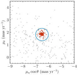
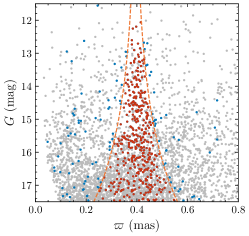
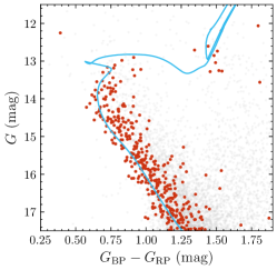
The clusters’ ages, distances and extinction values were estimated based on visual comparison with the MIST isochrones (Choi et al., 2016). The parameters of the best-fitting isochrone to the blue edge of the bulk stellar population of each cluster (Fig. 1, right) are included in Table 1. Our independently derived cluster parameters are consistent with literature values (e.g., Bossini et al., 2019); minor differences relate to the choice of stellar models adopted.
| Cluster | [Fe/H] | ||||||||
| (mag) | (dex) | (mag) | (mag) | ||||||
| (1) | (2) | (3) | (4) | (5) | (6) | (7) | (8) | (9) | (10) |
| NGC 3960 | 8.98 | 11.35 | 0.25 | 1.00 | |||||
| NGC 6134 | 8.96 | 10.28 | 0.08 | 1.32 | –a | ||||
| IC 4756 | 8.94 | 8.16 | 0.00 | 0.50 | –a | ||||
| NGC 5822 | 8.90 | 9.46 | 0.00 | 0.50 | |||||
| NGC 2818 | 8.89 | 12.56 | 0.00 | 0.60 | |||||
| a Insufficient sample size. | |||||||||
-
•
(1) Cluster name; (2) Age; (3) Distance modulus; (4) Metallicity; (5) Extinction; (6) Total binary fraction; (7) Scatter in pseudo-colour; (8) Slow-rotator number fraction among synthetic MSTO stars; (9, 10) Mass segregation ratios (MSRs) of (9) bMS and (10) rMS stars.
2.2 Spectroscopic data
For three -old Galactic OCs—NGC 3960, NGC 6134 and IC 4756—we obtained new medium-resolution spectroscopy. We expanded our sample by including NGC 5822 (Sun et al., 2019a) and NGC 2818 (Bastian et al., 2018). The first four of these clusters were observed in multi-object mode with the Robert Stobie Spectrograph on the Southern African Large Telescope (programmes 2017-2-SCI-038, 2018-1-SCI-006 and 2018-2-SCI-002), during 18 nights between 4 January 2018 and 26 April 2019.
The spectrograph configuration for our new observations was the same as that adopted by Sun et al. (2019a). The PG2300 grating was used at a grating angle of 34.25 degrees and a camera station angle of 68.5 degrees. This configuration, combined with a slit width of 1 arcsec, yields a central wavelength of 4884.4 Å and a spectral coverage of 4345–5373 Å at a resolving power of (the detector’s wavelength coverage also depends on the location of the slits). Argon lamp exposures and flat-field calibration frames were taken at the end of each observation for wavelength calibration and flat-field correction, respectively. We did not observe standard-star spectra, since flux calibration does not affect the line profiles of the Mg i triplets used for the rotational velocity estimation. Overscan correction, bias subtraction, gain correction and wavelength calibration were done using the PySALT package (Crawford et al., 2010). The exposure time was adjusted based on the average brightness of the stars in the mask to ensure a typical minimum signal-to-noise ratio (S/N) per pixel exceeding 200.
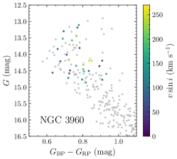
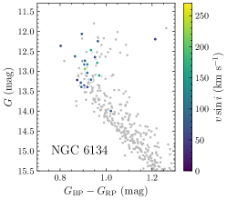
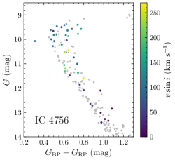
We determined the stars’ projected rotational velocities following Sun et al. (2019a) by fitting H and the Mg i triplet with the synthetic stellar spectra from the Pollux database (Palacios et al., 2010), convolved with the rotational profile for a given rotational velocity and implemented by adopting instrumental broadening. The error was estimated through a comparison of the rotational velocities of the mock data with those derived through profile fitting (Sun et al., 2019a, their figure 4). For IC 4756 we also included stellar rotation measurements from Schmidt & Forbes (1984) and Strassmeier et al. (2015). For stars with multi-epoch observations, a variability test indicated no significant variation of either the radial or the rotational velocities in our data set (except for one star in NGC 6134; see Section 4). As such, we adopted the average rotational velocity. We thus obtained rotation measurements of 29, 25 and 49 stars in NGC 3960, NGC 6134 and IC 4756, respectively. In Fig. 2, we present the CMDs of NGC 3960, NGC 6134 and IC 4756, with the member stars colour-coded by their rotational velocities. Combined with 24 stars in NGC 5822 and 57 in NGC 2818, we achieved 20–30 per cent completeness across the eMSTO for all five clusters. This is sufficient to reliably derive their rotation distributions (see Section 3.1.2).
2.3 Colour–magnitude diagram
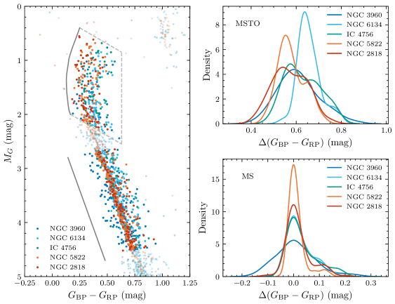
All sample clusters have similar chronological and dynamical ages (see Appendix A), thus enabling direct comparison upon correction of the clusters’ photometry for extinction and distance differences: see Fig. 3 (left). Whereas the clusters’ MSTOs exhibit different patterns, their lower MSs converge at approximately the same position in CMD space. We selected samples of MSTO and MS stars to better illustrate their morphologies using pseudo-colour distributions.
The selection boundaries applied to the MSTO stars are shown in Fig. 3 (grey enclosure): stars bluer than 0.63 mag and redder than the blue ridge line defined by the rotation model (see Section 3) were considered MSTO stars. The slopes of the cuts at the bright and faint ends follow the expected stellar locus change caused by stellar rotation. The pseudo-colour is defined as the difference in colour with respect to a cluster’s ridge line. We excluded a number of possible blue straggler stars at colours bluer than the best-fitting isochrone to the cluster’s bulk stellar population minus (see Section 3). Next, we defined a straight line parallel to the MS, at , as our MS reference. In Fig. 3 (right), KDEs of MSTO and MS stars are presented. The MS KDEs exhibit similar profiles, with a dominant peak at and a minor bump corresponding to the binary sequence redder than the peak. However, the MSTO KDEs exhibit significant variation both in the peak locations and the overall distributions.
3 Unravelling the rotation distributions
Several recent attempts have been made to unravel cluster rotation distributions (Gossage et al., 2019; de Juan Ovelar et al., 2020). However, most of these estimates were based solely on their CMD morphologies (see also Kamann et al., 2020), i.e., based on the probability of models matching the observations using Hess diagrams. Whereas this may be suitable for MC clusters, where the numbers of member stars are sufficiently large and where it is difficult or impossible to obtain direct velocity information, such analyses of OCs inevitably suffer from stochastic sampling effects (see Section 3.1.2). Spectroscopic observations can ameliorate these effects.
We used the SYCLIST stellar rotation models (Georgy et al., 2013, 2014) to generate synthetic clusters, assuming solar metallicity (), an age of and a 50 per cent binary fraction. The model also considers limb darkening (Claret, 2000). We adopted the gravity-darkening law of Espinosa Lara & Rieutord (2011). The inclination angles follow a random distribution. The model suite is limited to a minimum stellar mass of M⊙ and it does not account for the evolution of interacting binary systems.
Since the SYCLIST models are limited to high masses ( M⊙; suitable for covering the MSTO) and it is difficult to constrain a cluster’s binary fraction based on the morphology of its MSTO, we exploited the less massive MS stars (see Fig. 3) to derive total binary fractions, , at masses where the effects of stellar rotation are negligible. Binary models were generated from the MIST isochrones by adding unresolved binaries with different mass ratios, assuming a flat mass-ratio distribution. Next, we compared the pseudo-colour distributions of stars in our synthetic clusters with those in the observed clusters, using the same MS selection criteria. The goodness of the comparison is given by the Anderson–Darling value. We added a second parameter, , to characterise the observational scatter in the pseudo-colour, combining the effects of a possible internal age spread, photometric uncertainties and differential extinction. A minor colour shift among the clusters was also taken into consideration. We employed the Markov-chain Monte Carlo method (emcee; Foreman-Mackey et al., 2013) to determine the best model and estimate the uncertainties in the resulting parameters.
We adopted this binary fraction as our input parameter and applied a similar method to the MSTO stars to derive their rotation distribution. In the SYCLIST models, on the zero-age MS (ZAMS) this distribution is controlled by the ratio of the equatorial angular velocity, , to the critical velocity . The latter is the rotational angular velocity where the surface gravity can no longer maintain equilibrium with the centrifugal motion. We binned the resulting rotation rates into 10 bins, from to 1.0 in steps of 0.1, and assigned 10 weights, . Each weight corresponded to the fraction of stars with a given rotation rate.
We first generated a model cluster of 200,000 stars with a flat rotation distribution. For each set of input parameters (, ), we randomly selected the most appropriate stars from the total pool to generate a new synthetic cluster which satisfied the rotation distribution required. Subsequently, we added scatter () to the synthetic cluster and selected the remaining MSTO stars for comparison with the observed cluster. In practice, when selecting MSTO stars and calculating their pseudo-colours, we shifted the ridge line towards bluer colours by 0.3 mag to include MSTO stars which have scattered away from the MSTO region.
As for the MS region, a comparison of the pseudo-colour distributions of MSTO stars in the synthetic and observed clusters yields the corresponding values. We also used the rotational velocities to address the degeneracy between the pseudo-colour and rotation-velocity distributions (see Section 3.1.2). For each MSTO star with spectroscopic measurements, we selected the closest 100 stars in the synthetic cluster’s CMD. We then computed the probability of deriving the same distribution as observed. We first resampled the measured projected rotational velocities according to the error distribution and estimated the probabilities for this alternative realisation. We iterated each run 100 times and adopted the median value to minimise stochastic sampling effects. Finally, we combined the corresponding values from the spectroscopic data with and used emcee to find the rotation model which best reproduces both the pseudo-colour and the distributions. The uncertainties were derived from the samples’ 16th and 84th percentiles in the marginalised distributions.
3.1 Validation
In this section, we examine the accuracy of our parameter recovery, specifically for two crucial parameters, i.e., the binary fraction () and the rotation rate (). We discuss the importance of knowing the rotational velocity for the determination of the rotation distribution.
3.1.1 Binary fraction
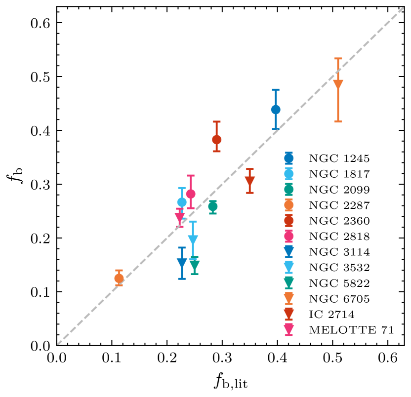
We applied our method to a few additional clusters to verify our calculation of the binary fraction. We selected 12 OCs with binary fraction measurements available in the literature (Bica & Bonatto, 2005; Cordoni et al., 2018; de Juan Ovelar et al., 2020) as our comparison sample. Given that these clusters are younger than or of similar age as our sample OCs, our selection of MS stars is not affected by any MSTO broadening and is thus suitable for validation purposes. In Fig. 4, we show our results (vertical axis) versus the corresponding literature mean values (horizontal axis). Considering possible differences in the sample selection and the estimation method used, our estimates for these OCs are consistent with the literature values
One possible flaw inherent to the derivation of binary fractions based on Gaia data is that some binaries could be (partially) resolved, which is not taken into account in the application of this method. If so, this would lead to an underestimation of the binary fraction and this could be important for clusters which are sufficiently close. However, this effect should not have a major impact on our sample clusters. Even for the nearest cluster analysed in this paper, IC 4756, only wide binaries with separations larger than (2 arcsec, adopted from Arenou et al., 2018) can be resolved by Gaia, which applies to less than 2 per cent of binaries in OCs (Deacon & Kraus, 2020).
3.1.2 Rotation rates
Verification of the rotation rates was done based on mock tests. We generated mock data for various rotation distributions and applied our method to verify whether the rotation rates were robustly recovered. In particular, we generated a synthetic cluster with 200 MSTO stars (similar to the observed number) and a spectroscopic completeness level of 25 per cent. The binary fraction and were set at 20 per cent and 0.02 mag, respectively.
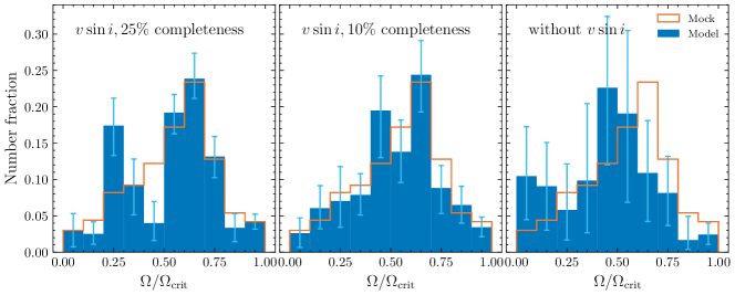
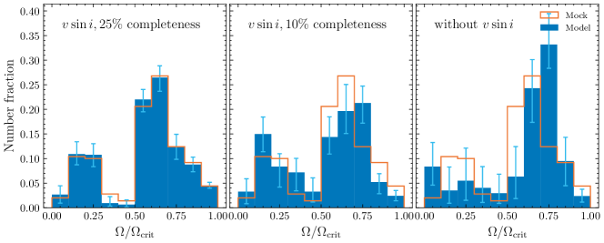
Fig. 5 shows two representations of our mock tests. One is based on a skewed normal distribution (first row) and the other is characterised by a bimodal distribution (second row). The input and recovered rotation rates are shown in the left-hand column as the orange and blue histograms, respectively. Our derived rotation rates are consistent with the mock data’s true values (most fall within ).
We also checked the performance of our approach in the presence of less or no spectroscopic information. The results for synthetic clusters with 10 and 0 per cent of information are shown in the middle and right-hand columns, respectively. The recovered rotation rates exhibit strong deviations from the input distribution. Although a general trend can tentatively still be produced, the corresponding accuracy is far from satisfactory. Although analyses of massive MC clusters solely based on photometric data are practical (e.g., Gossage et al., 2019), one should be careful when applying this approach to Galactic OCs. This final test highlights the degeneracy resulting from fitting models to poorly sampled data and underscores the need for additional information (such as measurements).
4 Results and Discussion
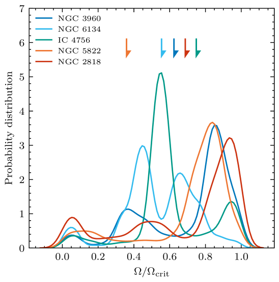
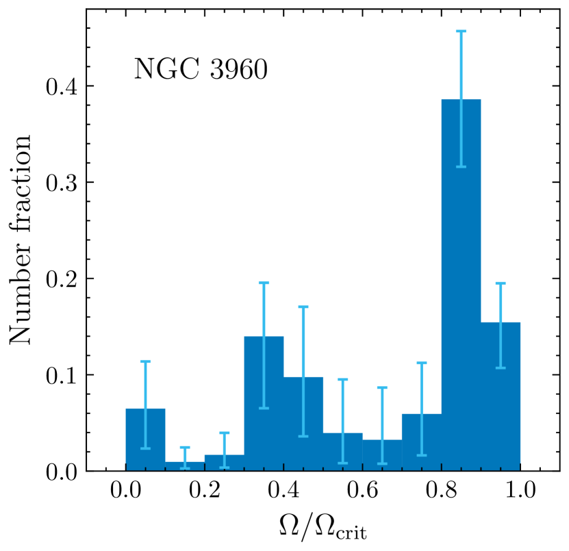
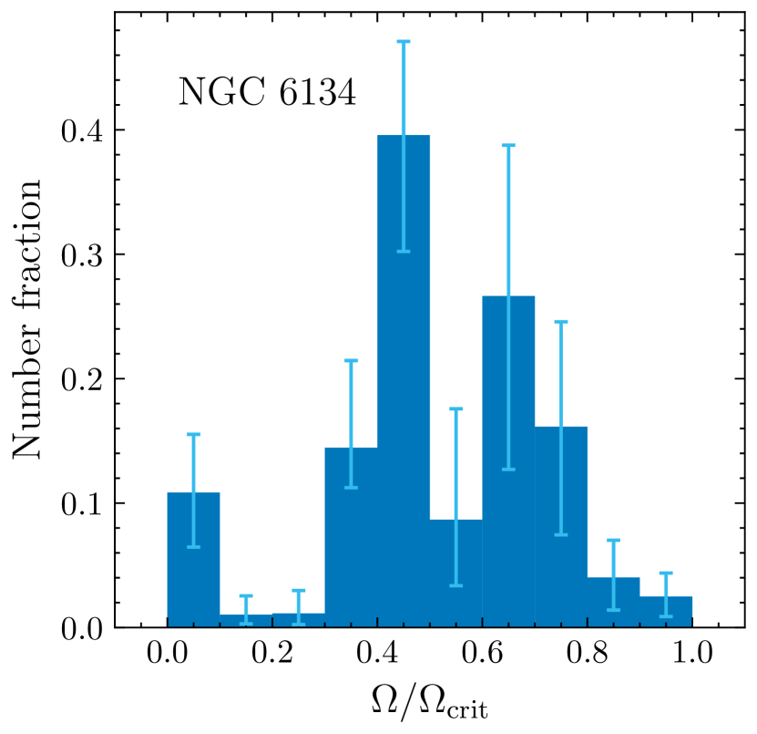
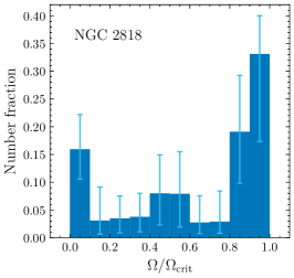
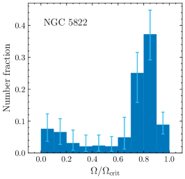
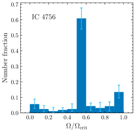
The best-fitting rotation rates’ weights are shown in Fig. 6 (small panels), whereas the rotation rate probability distributions of the MSTO stars for all clusters are shown in the top left-hand panel. All five clusters contain a significant fraction of fast rotators. However, the locations and fractions of fast rotators vary among the clusters. Whereas some clusters, like NGC 6134 and NGC 2818, appear to host three rotational populations (including two slowly rotating populations), it is difficult to reliably separate between populations of slow rotators because of their minor colour differences. Therefore, we exercise caution and suggest that these clusters may only contain two distinct populations (i.e., a bimodal distribution) in stellar rotation space.
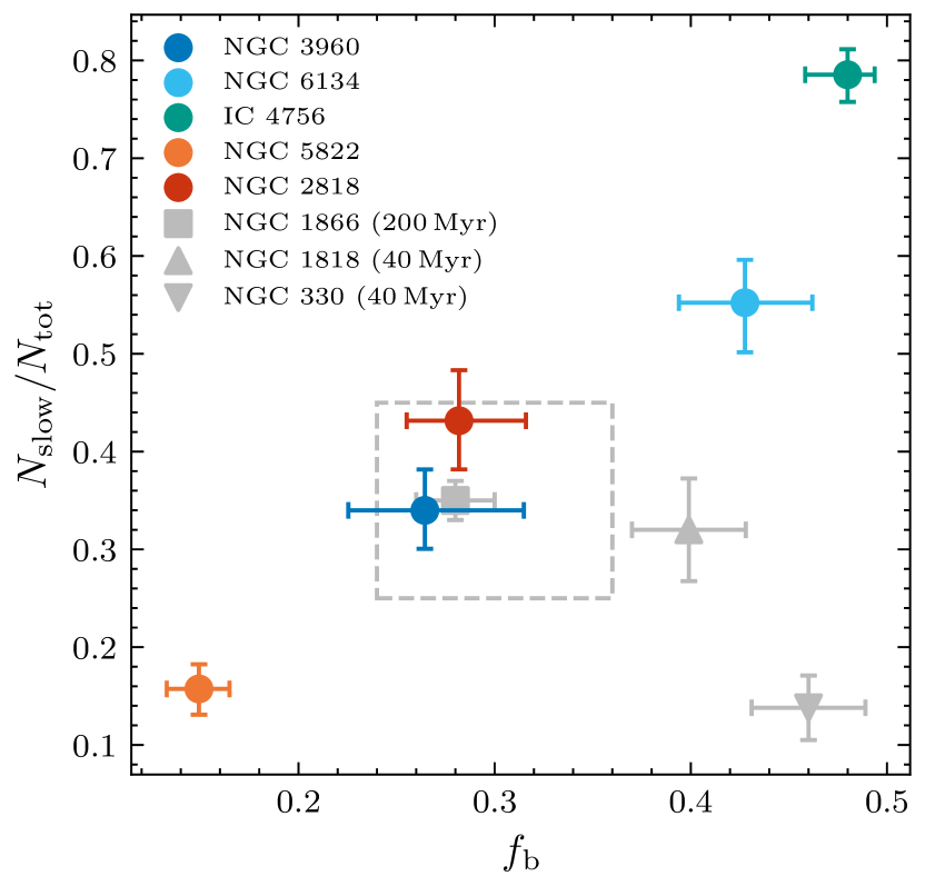
The number fraction of slow rotators, , among synthetic MSTO stars shows a positive correlation with the clusters’ total binary fraction : see Fig. 7. We verified that our approach to selecting slowly and rapidly rotating subsamples, within reasonable ranges, minimally affects this correlation by changing the velocity adopted for our subsample selection to fixed values. In all tests, the correlation between the number fraction of slow rotators and the binary fractions of the clusters remains almost the same, modulo minor shifts in the absolute value of In fact, one slow rotator () in NGC 6134 (Gaia DR2 ID 5941409684301615360) exhibited variation in its radial velocity during two observation epochs, spanning three days. The observed variation is around , which is four times larger than the uncertainty associated with the velocity measurements. The estimated rotational velocities remained unchanged, with differences of less than the error (). If this radial-velocity variation were induced by binaries, the star is likely a member of a close binary system with a separation of a few tens of solar radii. To arrive at this estimate, we assumed that its luminosity is not severely affected by the companion and we adopted the observed variation as the amplitude of radial velocity curve. Follow-up time-series observations are required to confirm this star’s nature.
The approximately constant number ratios of bMS stars found in massive MC clusters (Milone et al., 2018) may result from the similar binary fractions () which are prevalent in MC clusters (Milone et al., 2009) if the correlation of Fig. 7 also pertains to more massive clusters. For instance, Milone et al. (2017) estimated that the number ratio of bMS stars in NGC 1866 is 35 per cent; the cluster’s overall binary fraction is 0.28. These properties will place it comfortably on the apparent correlation. However, some younger clusters, e.g., NGC 1818 () and NGC 330 (), do not follow the correlation if we adopt their binary fractions from Li et al. (2017a) and their number ratios from Milone et al. (2018). This may suggest that these young clusters are still in the early stages of their stellar rotation evolution, which may last for several tens of Myr. In NGC 1846 (), Kamann et al. (2020) found that per cent of MSTO stars are slow rotators. They derived a binary fraction of 7 per cent based on radial velocity variations from four-epoch spectra. However, because their binary fraction measurement is limited by their temporal coverage and most sensitive to the detection of tight binaries, a large fraction of the cluster’s binaries are likely missing. Therefore, we did not include this cluster in Fig. 7.
To date, none of the prevailing theoretical models (e.g., D’Antona et al., 2015; Bastian et al., 2020) can naturally explain the observed correlation. Our observational result is in apparent conflict with the model of Bastian et al. (2020), which suggested that binaries may destroy stellar discs, thus resulting in faster rotational velocities on the MS. Moreover, this interpretation cannot explain the cluster-to-cluster variations in the MSTO pseudo-colour distributions in Fig. 3 (top right), which we verified using a two-sample Kolmogorov–Smirnov test. This is so, because our result is not an artefact of requiring a higher binary fraction to compensate for the potential narrowing of the MSTO owing to a lower fraction of fast rotators.
Neither does our correlation follow the scenario of D’Antona et al. (2015), where all or most stars form as fast rotators with a fraction undergoing close-binary tidal braking. Although this model predicts a larger fraction of slow rotators for a higher binary fraction, everything else being equal, the fraction of slow rotators can never exceed the binary fraction. Since only close binaries may become tidally locked, only a small subset of binaries could contribute. However, as shown in Fig. 7, the slow rotators’ number ratios are comparable to or even higher than the binary fractions. Moreover, the slope between and is close to unity regardless of the subsample selection, thus suggesting an alternative binary-driven mechanism. However, we cannot rule out a possible origin associated with the initial phase. The slow rotators we observe at the present time originate from both the initial population of slow rotators and may also have evolved from the fast rotators. Huang et al. (2010, their figure 7) selected a young subpopulation of B-type stars that just evolved from the zero-age main sequence and showed that a large fraction of them were formed as slow rotators. So far, it is unclear which physical property of (close and wide) binaries determines the rotation distributions. This may explain why Kamann et al. (2020) did not find any significant differences among the binary fractions of slow and fast rotators. If we consider the possibility of missing binaries from their sample, combined with the disruption of wide binaries, there could be distinct differences between slow and fast rotating populations.
If binaries are the dominant drivers of slow rotators, one would expect slow rotators to be more centrally concentrated in a cluster because they are generally more massive than their rapidly rotating counterparts, and they would thus sink more easily to the cluster centre owing to two-body relaxation (dynamical mass segregation; Binney & Tremaine, 1987). However, this scenario appears at odds with recent observations in young MC clusters. Dupree et al. (2017) and Milone et al. (2017) found that in NGC 1866 (), bMS stars (slow rotators) are less centrally concentrated than rMS stars (fast rotators). Meanwhile, in NGC 1856 (-old), the number ratios of bMS and rMS stars remain unchanged at different radii, thus suggesting that they are spatially homogeneously distributed (Li et al., 2017b).
We used the best-fitting synthetic cluster to infer the rotational velocities for all member stars (Sun et al., 2019a) and employed the spatial locations of the observed stars to estimate their degree of mass segregation. Because of their low number densities, it is hard to robustly determine the centres of OCs. Therefore, we adopted minimum spanning trees (MSTs) to quantify a cluster’s degree of mass segregation (Allison et al., 2009). The mass segregation ratio, , of a given population is defined as the ratio of the average random path length, , to that of the entire population, ,
| (2) |
where represents the length of the shortest path connecting all data points and quantifies the length distribution. We determined the OCs’ MSTs using MiSTree (Naidoo, 2019), in celestial coordinates. Given our OCs’ close proximity and the low stellar densities, the impact of sampling incompleteness of the low-mass stars in estimating is negligible.
To link our results with the observations of blue and red MSs, we adopted bMS stars as those stars with , whereas rMS stars have . This velocity threshold was selected based on the velocity dip at observed in NGC 1846 (Kamann et al., 2020). Given the mass differences of MSTO stars in clusters with different ages, this corresponds to for our sample. We assumed that the rotation rate () of the dip does not change for clusters of either 1 Gyr or 1.5 Gyr (NGC 1846). The critical rotation velocity only marginally decreases as a star evolves, whereas the rotation velocity strongly depends on stellar mass (Bastian et al., 2020, their figure 1). The typical MSTO stellar mass is around and for NGC 1846 and our cluster sample, respectively. Based on Georgy et al. (2014), the velocity dip for bMS and rMS should be 1.5 times larger in a 1 Gyr-old cluster than in NGC 1846.
The corresponding values are listed in Table 1. In all clusters, except for NGC 2818, the bMS stars exhibit significant spatial segregation, . Moreover, in NGC 3860 and NGC 5822, with differences . This suggests that the bMS stars in these clusters are more centrally concentrated than their rMS counterparts. This, hence, offers promising supporting evidence of a more massive origin of the bMS stars in these OCs. However, this is at odds with MC cluster results (e.g., Milone et al., 2017; Kamann et al., 2020). The difference could be attributed to binary disruption in the cluster centre. Milone et al. (2017) found the binary fraction to increase towards the cluster outskirts, following the same radial distribution as the bMS stars in NGC 1866, whereas this effect is not obvious in OCs.
In summary, we have discovered a strong observational correlation between the number ratios of the slow rotators and the binary fractions in five Galactic OCs and shown support for a marked concentration of bMS stars. Future work will extend the survey to younger clusters, cover a larger parameter space (e.g., in , stellar and cluster mass, metallicity, etc.) and study the detailed history of stellar rotation in cluster environments to gain additional important insights into the star cluster formation processes.
Acknowledgements
W.S. thanks Xiao-Wei Duan for insightful discussions. He is grateful for financial support from the China Scholarship Council. L.D. acknowledges research support from the National Natural Science Foundation of China through grants 11633005, 11473037 and U1631102. This work has made use of data from the European Space Agency (ESA) mission Gaia (http://www.cosmos.esa.int/gaia), processed by the Gaia Data Processing and Analysis Consortium (DPAC, http://www.cosmos.esa.int/web/gaia/dpac/consortium).
Data Availability
The data analysed in this paper will be shared upon request.
References
- Allison et al. (2009) Allison, R. J., Goodwin, S. P., Parker, R. J., et al. 2009, MNRAS, 395, 1449
- Arenou et al. (2018) Arenou, F., Luri, X., Babusiaux, C., et al. 2018, A&A, 616, A17. doi:10.1051/0004-6361/201833234
- Bastian et al. (2020) Bastian, N., Kamann, S., Amard, L., et al. 2020, MNRAS, 495, 1978. doi:10.1093/mnras/staa1332
- Bastian et al. (2018) Bastian, N., Kamann, S., Cabrera-Ziri, I., et al. 2018, MNRAS, 480, 3739. doi:10.1093/mnras/sty2100
- Bica & Bonatto (2005) Bica, E. & Bonatto, C. 2005, A&A, 431, 943. doi:10.1051/0004-6361:20042023
- Binney & Tremaine (1987) Binney, J. & Tremaine, S. 1987, Princeton, N.J. : Princeton University Press, c1987
- Bossini et al. (2019) Bossini, D., Vallenari, A., Bragaglia, A., et al. 2019, A&A, 623, A108. doi:10.1051/0004-6361/201834693
- Cantat-Gaudin et al. (2018) Cantat-Gaudin, T., Vallenari, A., Sordo, R., et al. 2018, A&A, 615, A49. doi:10.1051/0004-6361/201731251
- Choi et al. (2016) Choi, J., Dotter, A., Conroy, C., et al. 2016, ApJ, 823, 102. doi:10.3847/0004-637X/823/2/102
- Claret (2000) Claret, A. 2000, A&A, 359, 289
- Cordoni et al. (2018) Cordoni, G., Milone, A. P., Marino, A. F., et al. 2018, ApJ, 869, 139. doi:10.3847/1538-4357/aaedc1
- Crawford et al. (2010) Crawford, S. M., Still, M., Schellart, P., et al. 2010, Proc. SPIE, 7737, 773725. doi:10.1117/12.857000
- D’Antona et al. (2015) D’Antona, F., Di Criscienzo, M., Decressin, T., et al. 2015, MNRAS, 453, 2637. doi:10.1093/mnras/stv1794
- D’Antona et al. (2017) D’Antona, F., Milone, A. P., Tailo, M., et al. 2017, Nature Astronomy, 1, 0186. doi:10.1038/s41550-017-0186
- de Juan Ovelar et al. (2020) de Juan Ovelar, M., Gossage, S., Kamann, S., et al. 2020, MNRAS, 491, 2129. doi:10.1093/mnras/stz3128
- Deacon & Kraus (2020) Deacon, N. R. & Kraus, A. L. 2020, MNRAS, 496, 5176. doi:10.1093/mnras/staa1877
- Dupree et al. (2017) Dupree, A. K., Dotter, A., Johnson, C. I., et al. 2017, ApJ, 846, L1. doi:10.3847/2041-8213/aa85dd
- Espinosa Lara & Rieutord (2011) Espinosa Lara, F. & Rieutord, M. 2011, A&A, 533, A43. doi:10.1051/0004-6361/201117252
- Evans et al. (2018) Evans, D. W., Riello, M., De Angeli, F., et al. 2018, A&A, 616, A4. doi:10.1051/0004-6361/201832756
- Foreman-Mackey et al. (2013) Foreman-Mackey, D., Hogg, D. W., Lang, D., et al. 2013, PASP, 125, 306. doi:10.1086/670067
- Gaia Collaboration et al. (2018a) Gaia Collaboration, Babusiaux, C., van Leeuwen, F., et al. 2018a, A&A, 616, A10. doi:10.1051/0004-6361/201832843
- Gaia Collaboration et al. (2016) Gaia Collaboration, Brown, A. G. A., Vallenari, A., et al. 2016, A&A, 595, A2. doi:10.1051/0004-6361/201629512
- Gaia Collaboration et al. (2018b) Gaia Collaboration, Brown, A. G. A., Vallenari, A., et al. 2018b, A&A, 616, A1. doi:10.1051/0004-6361/201833051
- Georgy et al. (2013) Georgy, C., Ekström, S., Granada, A., et al. 2013, A&A, 553, A24. doi:10.1051/0004-6361/201220558
- Georgy et al. (2014) Georgy, C., Granada, A., Ekström, S., et al. 2014, A&A, 566, A21. doi:10.1051/0004-6361/201423881
- Gossage et al. (2019) Gossage, S., Conroy, C., Dotter, A., et al. 2019, ApJ, 887, 199. doi:10.3847/1538-4357/ab5717
- Goudfrooij et al. (2011) Goudfrooij, P., Puzia, T. H., Kozhurina-Platais, V., et al. 2011, ApJ, 737, 3. doi:10.1088/0004-637X/737/1/3
- Hoppe et al. (2020) Hoppe, R., Bergemann, M., Bitsch, B., et al. 2020, A&A, 641, A73. doi:10.1051/0004-6361/20193693
- Huang et al. (2010) Huang, W., Gies, D. R., & McSwain, M. V. 2010, ApJ, 722, 605. doi:10.1088/0004-637X/722/1/605
- Kamann et al. (2020) Kamann, S., Bastian, N., Gossage, S., et al. 2020, MNRAS, 492, 2177. doi:10.1093/mnras/stz3583
- Li et al. (2017a) Li, C., de Grijs, R., Deng, L., et al. 2017a, ApJ, 844, 119. doi:10.3847/1538-4357/aa7b36
- Li et al. (2017b) Li, C., de Grijs, R., Deng, L., et al. 2017b, ApJ, 834, 156. doi:10.3847/1538-4357/834/2/156
- Mackey & Broby Nielsen (2007) Mackey, A. D. & Broby Nielsen, P. 2007, MNRAS, 379, 151. doi:10.1111/j.1365-2966.2007.11915.x
- Meylan (1987) Meylan, G. 1987, A&A, 184, 144
- Milone et al. (2009) Milone, A. P., Bedin, L. R., Piotto, G., et al. 2009, A&A, 497, 755. doi:10.1051/0004-6361/200810870
- Milone et al. (2017) Milone, A. P., Marino, A. F., D’Antona, F., et al. 2017, MNRAS, 465, 4363. doi:10.1093/mnras/stw2965
- Milone et al. (2018) Milone, A. P., Marino, A. F., Di Criscienzo, M., et al. 2018, MNRAS, 477, 2640. doi:10.1093/mnras/sty661
- Naidoo (2019) Naidoo, K. 2019, The Journal of Open Source Software, 4, 1721. doi:10.21105/joss.01721
- Niederhofer et al. (2015) Niederhofer, F., Georgy, C., Bastian, N., et al. 2015, MNRAS, 453, 2070. doi:10.1093/mnras/stv1791
- Palacios et al. (2010) Palacios, A., Gebran, M., Josselin, E., et al. 2010, A&A, 516, A13. doi:10.1051/0004-6361/200913932
- Schmidt & Forbes (1984) Schmidt, E. G. & Forbes, D. 1984, MNRAS, 208, 83. doi:10.1093/mnras/208.1.83
- Soubiran et al. (2018) Soubiran, C., Cantat-Gaudin, T., Romero-Gómez, M., et al. 2018, A&A, 619, A155. doi:10.1051/0004-6361/201834020
- Strassmeier et al. (2015) Strassmeier, K. G., Weingrill, J., Granzer, T., et al. 2015, A&A, 580, A66. doi:10.1051/0004-6361/201525756
- Sun et al. (2019a) Sun, W., de Grijs, R., Deng, L., et al. 2019a, ApJ, 876, 113. doi:10.3847/1538-4357/ab16e4
- Sun et al. (2019b) Sun, W., Li, C., Deng, L., et al. 2019b, ApJ, 883, 182. doi:10.3847/1538-4357/ab3cd0
- Wu et al. (2016) Wu, X., Li, C., de Grijs, R., et al. 2016, ApJ, 826, L14. doi:10.3847/2041-8205/826/1/L14
- Yang et al. (2013) Yang, W., Bi, S., Meng, X., et al. 2013, ApJ, 776, 112. doi:10.1088/0004-637X/776/2/112
Appendix A Dynamical timescale
Dynamical modelling of OCs is rendered uncertain by the small numbers of their member stars. To derive approximate dynamical ages for our sample OCs, we calculated their half-mass relaxation time-scales (Meylan, 1987),
| (3) |
where is the half-mass radius derived from number counts, is the total mass derived following Sun et al. (2019a) and is the typical mass of stars in the cluster. This estimate yields relatively similar half-mass relaxation time-scales for all of our sample OCs, ranging from to . We double checked this result by comparison with Binney & Tremaine (1987)
| (4) |
where is the crossing time, is the total number of stars and is the velocity dispersion. We adopted the latter from Soubiran et al. (2018). Both estimates are in reasonable mutual agreement, in the sense that the clusters’ dynamical time-scales are around 100 Myr, varying by a factor of up to 2. This means that our clusters have evolved through approximately 9–16 half-mass relaxation time-scales and share similar dynamical ages.