Biolocomotion and premelting in ice

Jérémy Vachier jeremy.vachier@su.se Nordita, KTH Royal Institute of Technology and Stockholm University, Hannes Alfvéns väg 12, SE-106 91 Stockholm, Sweden J. S. Wettlaufer john.wettlaufer@yale.edu Nordita, KTH Royal Institute of Technology and Stockholm University, Hannes Alfvéns väg 12, SE-106 91 Stockholm, Sweden Yale University, New Haven, Connecticut 06520-8109, USA

Abstract

Biota are found in glaciers, ice sheets and permafrost. Ice bound micro-organisms evolve in a complex mobile environment facilitated or hindered by a range of bulk and surface interactions. When a particle is embedded in a host solid near its bulk melting temperature, a melted film forms at the surface of the particle in a process known as interfacial premelting. Under a temperature gradient, the particle is driven by a thermomolecular pressure gradient toward regions of higher temperatures in a process called thermal regelation. When the host solid is ice and the particles are biota, thriving in their environment requires the development of strategies, such as producing exopolymeric substances (EPS) and antifreeze glycoproteins (AFP) that enhance the interfacial water. Therefore, thermal regelation is enhanced and modified by a process we term bio-enhanced premelting. Additionally, the motion of bioparticles is influenced by chemical gradients influenced by nutrients within the icy host body. We show how the overall trajectory of bioparticles is controlled by a competition between thermal regelation and directed biolocomotion. By re-casting this class of regelation phenomena in the stochastic framework of active Ornstein-Uhlenbeck dynamics, and using multiple scales analysis, we find that for an attractive (repulsive) nutrient source, that thermal regelation is enhanced (suppressed) by biolocomotion. This phenomena is important in astrobiology, the biosignatures of extremophiles and in terrestrial paleoclimatology.

^†^†preprint: APS/123-QED

I Introduction

Ice sheets are an essential reservoir of information on past climate and they contain an important record of micro-organisms on Earth, recording ice microbes and their viruses over long periods [1, 2]. In these extreme environments, the abundance of virus is well correlated with bacterial abundance, but is 10 to 100 times lower than in temperate aquatic ecosystems [3]. Even in these harsh conditions, the virus infection rate is relatively high [4], leading to the expectation of low long-term survival rates. However, recent studies have shown that some viruses develop survival strategies to maintain a long-term relationship with their hosts [4, 5], possibly up to thousands of years [6]. For example, viruses such as bacteriophages can switch to a lysogenic life strategy enabling them to replicate and maintain themselves in the bacterial population without lysis over multiple generations [4]. Moreover, among these viruses some can provide immunity to their hosts against other viruses [4, 7], or manipulate their metabolism to facilitate nutrient acquisition by affecting motility genes [6]. Indeed, motile biota are found to be active in ice for substantial periods. For example, recently a 30,000 year old giant virus Pithovirus sibericum was found in permafrost [8] along with microbes [9, 10] and nematodes [11], and viable bacteria have been found in 750,000 year old glacial ice [12]. Basal ice often contains subglacial debris and sediment, which serve as a source of nutrients and organic matter, providing a habitat for micro-organisms adapted to subfreezing conditions [13, 14]. Additionally, the microbiomes of sediment rich basal ices are distinct from those found in glacial ice and are equivalent to those found in permafrost [13], expanding the nature of subfreezing habitats.
Ice cores provide the highest resolution records of past climate states [e.g., 15, 16, 17, 18, 19, 20]. Of particular relevance to our study is their role as a refuge for micro-organisms, from the recent past [21, 22] to millennia [23, 24, 25]. Ice microbes are taxonomically diverse and have a wide range of taxonomic relatives [14, 26, 27, 28, 24]. Common algae taxa are centric and pennate diatoms, dinoflagellates and flagellates [29, 30, 31], whereas common bacterial taxa are pseudomonadota, actinobacteria, firmicutes and bacteroidetes [6, 32]. Many of these microbes have different motility mechanisms [33, 34] from swimming (e.g., Chlamydomonas nivalis [35] or Methylobacterium [36, 37, 6]) to gliding (e.g., diatoms [38, 39] or Bacillus subtilis [24, 40]), which can be used to assess their locomotion. Examples of biological proxies include diatoms [41] and bacteria colonies [42, 43], reflecting a unique range of physical-biological interactions in the climate system. Therefore, understanding the relationship between the evolution of ice bound micro-organisms and proxy dating methods is a key aspect of understanding the covariation of life and climate.
Finally, such understanding is essential for the study of extraterrestrial life. In our own solar system, despite the debate regarding the existence of bulk water on Mars [e.g., 44], thin water films, such as those studied here, hold the most potential for harboring life under extreme conditions. Indeed, lipids, nucleic acids, and amino acids influenced by active motility may serve as biosignatures of extra terrestial life. Combining measurements of diffusivity-characterized-motility [45, 46] with bioparticle distribution observed on Earth, provides crucial information for development of new instrumentation to detect the presence of extra terrestrial life [46, 47]. Indeed, recently micro-organisms trapped in primary fluid inclusions in halite for millions of years have been discovered [48], providing promise for both terrestrial and extraterrestrial biosignature detection.

Refer to caption — Figure 1: Schematic of few active particles embedded in ice under an external temperature gradient $\nabla T$ along the $\tilde{z}$ -axis. The nutrient source is shown by the purple gradient. The external temperature gradient induces a drift velocity, and particles move toward regions of higher temperature, in a process known as thermal regelation (black arrow). An additional drift velocity is associated with particle motion towards higher concentration of nutrients (black dotted arrow). Thus, depending on a particle’s position, and the background temperature and nutrient gradients, these two drift effects can compete or amplify each other.

When a particle is embedded in ice near the bulk melting temperature, the ice may melt at the particle-ice surface in a process known as interfacial premelting [49]. The thickness of the melt film depends on the temperature, impurities, material properties and geometry. A temperature gradient is accompanied by a thermomolecular pressure gradient that drives the interfacial liquid from high to low temperatures, and hence the particle migrates from low to high temperatures in a process called thermal regelation [50, 49, 51, 52, 53]. Thermal regelation of inert particles plays a major role in the redistribution of material inside of ice, which has important environmental and composite materials implications [50, 49, 51, 52, 53]. Moreover, surface properties are central to the fact that extremophile organisms in Earth’s cryosphere–glaciers, sea ice and permafrost–develop strategies to persist in challenging environments. Indeed, many biological organisms secrete exopolymeric substance (EPS) [54] or harness antifreeze glycoproteins (AFP) [55, 56] to maintain interfacial liquidity. For example, sea ice houses an array of algae and bacteria, some of which produce EPS to protect them at low temperature and high salinity [57, 58]. Additionally, the enhanced liquidity associated with high concentrations of EPS alters the physical properties of sea ice and thereby play a role in climate change [59, 60].
In bulk solution, active particles act as simple microscopic models for living systems and are particularly accurate at mimicking the propulsion of bacteria or algae [e.g., 61, 62, 63, 64, 65]. By converting energy to motion using biological, chemical, or physical processes, they exhibit rich collective emergent motion from ostensibly simple rules [e.g., 66, 67]. Algae and bacteria operate in complex geometries and translate environmental conditions into microscopic information that guides their behavior. Examples of such information include quorum sensing (e.g., particle population density), used by bacteria to regulate biofilm formation, defense against competitors and adapt to changing environments [68, 69, 70]; chemotaxis (e.g., concentration gradients of nutrients), used by algae/bacteria to direct their motion toward higher concentrations of beneficial, or lower concentrations of toxic, chemicals [71, 72, 73, 74, 75]. It is important to emphasize that factors such as surface adhesion, salinity, the segregation of impurities of all types from the ice lattice, among other factors [See e.g., 76, 77, 74, 78], make our treatment of chemotaxis a simplified starting point. However, field samples and laboratory experiments have shown that cell motility is influenced by chemotaxis at low temperature [79, 45, 80]. Thus, although there are many complicated interactions that provide scope for future work, the basic role of chemotaxis in the distribution of biota in ice must start with a self-consistent framework, which is the focus of our work.
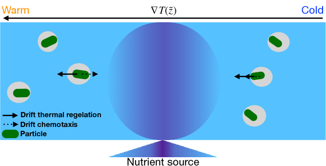
The confluence of thermal regelation, bio-enhanced premelting and intrinsic mobility underlie our study. Indeed, intrinsic mobility and chemotaxis may compete with thermal regelation, which constitutes a new area of research–ice bound active particles in premelting ice, as illustrated in Fig. 1. Moreover, including micro-organism protection mechanisms that enhance interfacial liquidity, such as the secretion of EPS, constitute a unique class of regelation phenomena. Finally, treating this corpus of processes quantitatively is particularly relevant for climatology and the global carbon cycle [e.g., 81, 82].
Our framework is the active Ornstein-Uhlenbeck particle (AOUP) [e.g 83, 84, 85, 86, 87, 88, 89]. The active force is governed by an Ornstein-Uhlenbeck process with magnitude $\tilde{D}_{a}$ , which is the active diffusivity. This force can be compared to a colored noise process [85, 90]. In addition to the active diffusivity, the AOUP is characterized by a time $\tau_{a}$ , which defines the noise persistence, from which the system switches from a ballistic to a diffusive regime. The active diffusivity $\tilde{D}_{a}$ and characteristic time $\tau_{a}$ can be measured experimentally [91, 92, 93]. The AOUP has been shown to provide accurate predictions for a range of complex phenomena [94, 84, 87, 86], and is theoretically advantageous due to its Gaussian nature [85]. These issues motivate our use of the AOUP model framework to describe the motion of active particles in ice under an external temperature gradient with a nutrient source. We analyze these particles in three dimensions using a multiple scale expansion to derive the associated Fokker-Planck equation.
The paper is organized as follows. In order to make our treatment reasonably self-contained we note that we are generalizing our previous approach [53, 95], which we recover in the appropriate limit. Thus, in §II we introduce the active Ornstein-Uhlenbeck model for bio-premelted particles and in §III we derive the associated Fokker-Planck equation using a multiple scale expansion. We then compare our analytic and numerical solutions after which, in §IV, we draw conclusions.

II Methods

Thermal regelation is understood as a consequence of the premelted film around a particle, originally treated as inert, that (a) executes diffusive motion in the ice column with diffusivity $\tilde{D}(\tilde{z})\mathbb{I}$ , where $\mathbb{I}$ is the identity matrix, and (b) experiences a drift velocity $\tilde{v}(\tilde{z})=U(\tilde{z})\hat{\tilde{\bm{z}}}$ parallel to the temperature gradient [53]. Therefore, regelation biases the motion of an active particle by the drift velocity $U(\tilde{z})\hat{\tilde{\bm{z}}}$ .
For inert particles with a sufficiently large number of moles of electrolyte impurities per unit area of surface, $N_{i}$ , the premelted film thickness $d\propto N_{i}$ [96, 53]. However, the production of EPS/AFP enhances liquidity at the ice surface by increasing the impurity concentration [59, 97, 77, 14], which we treat here using an enhancement factor as $N=nN_{i}$ , which gives

d=\frac{R_{g}T_{m}^{2}N}{\rho_{l}q_{m}\Delta T}\,,

(1)

where the universal gas constant is $R_{g}$ , the latent heat of fusion per mole of the solid is $q_{m}$ , the molar density of the liquid is $\rho_{l}$ , the undercooling is $\Delta T=T_{m}-T$ with $T_{m}=273.15$ K the pure bulk melting temperature and $T$ the temperature of ice.
The velocity and premelting-controlled diffusivity are given by

U(\tilde{z})=-\frac{A_{3}}{A_{2}^{3}}\frac{1}{\tilde{z}^{3}}\,\qquad\text{and}

(2)

\tilde{D}(\tilde{z})=\frac{(R_{g}T_{m}N)^{3}}{8\pi\nu R^{4}A_{2}^{3}}\frac{k_{B}T_{m}}{\tilde{z}^{3}}\,,

(3)

respectively, where $A_{2}=\rho_{l}q_{m}\frac{|\nabla T|}{T_{m}}$ and $A_{3}=\rho_{s}q_{m}|\nabla T|\frac{(R_{g}T_{m}N)^{3}}{6\nu RT_{m}}$ , with $|\nabla T|$ the external temperature gradient. The viscosity of the fluid is $\nu$ , the particle radius is $R$ and $k_{B}$ is the Boltzmann constant. Here, $\rho_{s}q_{m}\sim 334\times 10^{6}$ J m^-3 [53]. The evolution of the particle position $\tilde{\bm{r}}=(\tilde{r}_{1},\tilde{r}_{2},\tilde{r}_{3})=(\tilde{x},\tilde{y},\tilde{z})$ and its activity are described by two overdamped Langevin equations

	$\displaystyle\frac{d}{d\tilde{t}}\tilde{\bm{r}}(\tilde{t})$	$\displaystyle=\beta_{D}\nabla_{\tilde{\bm{r}}}\tilde{\mathcal{C}}(\tilde{\bm{r}},\tilde{t})+\sqrt{2\tilde{D}_{a}}\tilde{\bm{\eta}}+\tilde{v}(\tilde{z})+\sqrt{2\tilde{D}(\tilde{z})}\bm{\xi}_{p}(\tilde{t})\qquad\text{and}$		(4)
	$\displaystyle\frac{d}{d\tilde{t}}\tilde{\bm{\eta}}(\tilde{t})$	$\displaystyle=-\frac{1}{\tau_{a}}\tilde{\bm{\eta}}(\tilde{t})+\frac{1}{\tau_{a}}\bm{\xi}_{a}(\tilde{t})\,.$		(5)

The first term on the right-hand side of Eq. (4) treats the chemotaxis response, representing the effect of the nutrient source of concentration $\tilde{\mathcal{C}}$ on the particle dynamics, where $\beta_{D}$ is the chemotactic strength [98, 99, 100, 101], which we treat as a constant determined by the parameters in our system. We note, however, that the transport properties of sea- and glacial-ice depend on their unique phase fraction evolution [e.g. 102, 103, 104, 105], which would clearly influence the effective–porosity dependent $\beta_{D}$ . In the ideal case, wherein the nutrient source is isotropic and purely diffusive, we have

\frac{\partial}{\partial\tilde{t}}\tilde{\mathcal{C}}(\tilde{\bm{r}},\tilde{t})=\tilde{D}_{ch}\nabla^{2}_{\tilde{\bm{r}}}\tilde{\mathcal{C}}(\tilde{\bm{r}},\tilde{t})\,,

(6)

where $\tilde{D}_{ch}$ is the nutrient diffusivity. The activity, or self-propulsion, is given by the term $\sqrt{2\tilde{D}_{a}}\tilde{\bm{\eta}}$ in Eq. (4), with $\tilde{D}_{a}$ the active diffusivity. The latter represents the active fluctuations of the system, such as those originating in particular processes described in Refs. [106, 107, 108, 109]. Nutrient sources, such as dissolved silica, oxygen, nitrogen and methane, play a vital role in the life of ice-bound micro-organisms, such as algae and bacteria [e.g., 110, 111, 112, 113, 114, 115]. Here we assume that $\tilde{D}_{ch}>\tilde{D}_{a}$ , consistent with [116, 117, 118], and $\tilde{D}_{ch}>\tilde{D}(\tilde{z})$ . The function $\tilde{\bm{\eta}}=(\tilde{\eta}_{1},\tilde{\eta}_{2},\tilde{\eta}_{3})$ is described by an Ornstein-Uhlenbeck process, with correlations given by

\langle\tilde{\eta_{i}}(\tilde{t}^{\prime})\tilde{\eta_{j}}(\tilde{t})\rangle=\frac{\delta_{ij}}{{2}\tau_{a}}e^{-\frac{|\tilde{t}^{\prime}-\tilde{t}|}{\tau_{a}}}\,,

(7)

where $\tau_{a}$ is the noise persistence as noted above. In the small $\tau_{a}$ limit, $\tilde{\bm{\eta}}$ reduces to Gaussian white noise with correlations $\langle\tilde{\eta}_{i}(t^{\prime})\tilde{\eta}_{j}(t)\rangle=\delta_{ij}\delta(\tilde{t}^{\prime}-\tilde{t})$ . In contrast, $\tilde{\bm{\eta}}$ does not reduce to Gaussian white noise when $\tau_{a}$ is finite, and Eq. (4) does not reach equilibrium. Hence, $\tau_{a}$ controls the non-equilibrium properties of the dynamics [85, 86]. Finally, the random fluctuations in Eqs. (4) and (5) are given by zero mean Gaussian white noise processes $\langle\xi_{p_{i}}(\tilde{t}^{\prime})\xi_{p_{j}}(\tilde{t})\rangle=\delta_{ij}\delta(\tilde{t}^{\prime}-\tilde{t})$ and $\langle\xi_{a_{i}}(\tilde{t}^{\prime})\xi_{a_{j}}(\tilde{t})\rangle=\delta_{ij}\delta(\tilde{t}^{\prime}-\tilde{t})$ .
The Langevin Eqs. (4) and (5), allow us to express the probability of finding a particle at the position $\tilde{\bm{r}}=(\tilde{r}_{1},\tilde{r}_{2},\tilde{r}_{3})=(\tilde{x},\tilde{y},\tilde{z})$ at a given time $\tilde{t}$ through the Fokker-Planck equation, which describes the evolution of the probability density function $P(\tilde{\bm{r}},\tilde{\bm{\eta}},\tilde{t}|\tilde{\bm{r}}_{0},\tilde{\bm{\eta}}_{0},\tilde{t}_{0})$ , with the initial condition $P(\tilde{\bm{r}},\tilde{\bm{\eta}},\tilde{t}=\tilde{t}_{0}|\tilde{\bm{r}}_{0},\tilde{\bm{\eta}}_{0},\tilde{t}_{0})=\delta(\tilde{\bm{r}}-\tilde{\bm{r}}_{0})\delta(\tilde{\bm{\eta}}-\tilde{\bm{\eta}}_{0})$ . To simplify the notation, we write the conditional probability as $P(\tilde{\bm{r}},\tilde{\bm{\eta}},\tilde{t}|\tilde{\bm{r}}_{0},\tilde{\bm{\eta}}_{0},\tilde{t}_{0})\equiv P(\tilde{\bm{r}},\tilde{\bm{\eta}},\tilde{t})$ and eventually arrive at the following system of coupled equations,

$\displaystyle\frac{\partial}{\partial\tilde{t}}P(\tilde{\bm{r}},\tilde{\bm{\eta}},\tilde{t})$	$\displaystyle=-\beta_{D}\nabla_{\tilde{\bm{r}}}{\cdot}\left[P(\tilde{\bm{r}},\tilde{\bm{\eta}},\tilde{t})\nabla_{\tilde{\bm{r}}}\tilde{\mathcal{C}}(\tilde{\bm{r}},\tilde{t})\right]-\frac{\partial}{\partial\tilde{r}_{3}}\left[\tilde{v}(\tilde{r}_{3})P(\tilde{\bm{r}},\tilde{\bm{\eta}},\tilde{t})\right]-\sqrt{2\tilde{D}_{a}}\tilde{\bm{\eta}}\cdot\nabla_{\tilde{\bm{r}}}P(\tilde{\bm{r}},\tilde{\bm{\eta}},\tilde{t})$
	$\displaystyle+\nabla^{2}_{\tilde{\bm{r}}}\left[\tilde{D}(\tilde{r}_{3})P(\tilde{\bm{r}},\tilde{\bm{\eta}},\tilde{t})\right]+\frac{1}{\tau_{a}}\nabla_{\tilde{\bm{\eta}}}\cdot\left[\tilde{\bm{\eta}}P(\tilde{\bm{r}},\tilde{\bm{\eta}},\tilde{t})\right]+\frac{1}{2\tau_{a}^{2}}\nabla^{2}_{\tilde{\bm{\eta}}}P(\tilde{\bm{r}},\tilde{\bm{\eta}},\tilde{t})\qquad\text{and}$	(8)
$\displaystyle\frac{\partial}{\partial\tilde{t}}\tilde{\mathcal{C}}(\tilde{\bm{r}},\tilde{t})$	$\displaystyle=\tilde{D}_{ch}\nabla^{2}_{\tilde{\bm{r}}}\tilde{\mathcal{C}}(\tilde{\bm{r}},\tilde{t})\,.$	(9)

Equations (II) and (9) describe the space-time evolution of the probability of finding a particle and the concentration of nutrients respectively, akin to those of [83, 85, 119], but including the effects of thermal regelation discussed above. Both equations contain microscopic and macroscopic scales. The regime of interest is the long time behavior, computed by deriving the effective macroscopic dynamics as described next.

III Results

III.1 Method of multiple scales

The macroscopic length characterizing the heat flux is

L=\frac{T_{m}}{|\nabla T|}\,.

(10)

The particle scale $l$ is such that $l<<L$ , and hence their ratio defines a small parameter $\epsilon$

\epsilon=\frac{l}{L}\,.

(11)

We use the microscopic length $l$ and a characteristic time $\tau$ , determined a posteriori, and introduce the following dimensionless variables

\displaystyle\bm{\eta}=\sqrt{\tau_{a}}\tilde{\bm{\eta}}\text{, }\bm{r}=\frac{\tilde{\bm{r}}}{l}\text{, }t=\frac{\tilde{t}}{\tau}\text{, }v=\frac{\tilde{v}}{u}\text{, }v_{a}=\frac{\tilde{v}_{a}}{v_{ac}}\text{, }D=\frac{\tilde{D}}{D_{c}}\text{, }D_{ch}=\frac{\tilde{D}_{ch}}{D_{n}}\text{~{}and~{}}\mathcal{C}=\frac{\tilde{\mathcal{C}}}{c_{h}}\,,

(12)

where $\tilde{v}_{a}=\sqrt{\frac{2\tilde{D}_{a}}{\tau_{a}}}$ [120, 121], $v_{ac}$ is the characteristic active velocity, $u$ and $D_{c}$ are the characteristic values of the regelation velocity and the premelting enhanced diffusivity respectively, and $D_{n}$ and $c_{h}$ are the characteristic values of the diffusivity and nutrient concentration respectively. With these scalings, Eqs. (II) and (9), become

$\displaystyle P_{l}\frac{\partial}{\partial t}P$	$\displaystyle=-\beta_{D}\frac{c_{h}}{D_{c}}\nabla_{\bm{r}}\cdot\left[P\nabla_{\bm{r}}\mathcal{C}\right]-P_{e}\frac{\partial}{\partial r_{3}}\left[vP\right]-P_{a}v_{a}\bm{\eta}\cdot\nabla_{\bm{r}}P$	$\displaystyle+\nabla^{2}_{\bm{r}}\left[DP\right]+P_{A}\nabla_{\bm{\eta}}\cdot\left[\bm{\eta}P\right]+\frac{1}{2}P_{A}\nabla^{2}_{\bm{\eta}}P$	(13)
and			(14)
$\displaystyle P_{ch}\frac{\partial}{\partial t}\mathcal{C}$	$\displaystyle=D_{ch}\nabla^{2}_{r}\mathcal{C}\,,$		(15)

in which we have the following dimensionless numbers,

P_{e}=\frac{ul}{D_{c}}\text{, }P_{a}=\frac{v_{ac}l}{D_{c}}\text{, }P_{l}=\frac{l^{2}}{D_{c}\tau}\text{, }P_{A}=\frac{l^{2}}{D_{c}\tau_{a}}\text{ and }P_{ch}=\frac{l^{2}}{D_{n}\tau}\,.

(16)

We identify four characteristic time scales: $t_{l}^{\text{diff}}=l^{2}/D_{c}$ , $t_{l}^{\text{adv}}=l/u$ , $t_{L}^{\text{diff}}=L^{2}/D_{c}$ and $t_{L}^{\text{adv}}=L/u$ , associated with “microscopic” diffusion and advection on the particle scale, $l$ , and “macroscopic” diffusion and advection over the thermal length scale, $L$ . Nutrient and premelting enhanced diffusivity are taken to operate on the same time scale; $t^{\text{diff}_{n}}_{l,L}\sim t^{\text{diff}}_{l,L}$ . The Péclet number represents the ratio of the characteristic time for diffusion to that of advection, and those associated with regelation and activity are $P_{e}$ and $P_{a}$ respectively, and can be defined over both length scales,

P_{e}=\frac{t_{l}^{\text{diff}}}{t_{l}^{\text{adv}}}\qquad\text{ and }\qquad P_{e}^{L}=\frac{t_{L}^{\text{diff}}}{t_{L}^{\text{adv}}}\,.

(17)

The temperature gradient across the entire system drives thermal regelation and hence advection dominates on the macroscopic scale, so that $P_{e}^{L}=\mathcal{O}(1/\epsilon)$ , or equivalently, $t_{L}^{\text{adv}}=\epsilon t_{L}^{\text{diff}}\sim\epsilon t_{L}^{\text{diff}_{n}}$ . Whence, $P_{e}=\mathcal{O}(1)$ , or equivalently, $t_{l}^{\text{adv}}=t_{l}^{\text{diff}}\sim t_{l}^{\text{diff}_{n}}$ . On the macroscopic scale $P_{e}^{L}$ becomes large, as $\epsilon$ tends to zero, and thus we use the macroscopic advection time $\tau=t_{L}^{\text{adv}}$ as our characteristic time, so that Péclet numbers based on $L$ are $\mathcal{O}(1/\epsilon)$ and those based on $l$ are $\mathcal{O}(\epsilon)$ . In consequence, Eqs. (13) and (15) become leading to $P_{L}=\mathcal{O}(1/\epsilon)$ and $P_{l}=\mathcal{O}(\epsilon)$ , as well as $P^{ch}_{L}=\mathcal{O}(1/\epsilon)$ and $P^{ch}_{l}=\mathcal{O}(\epsilon)$ . The system of Fokker-Planck equations, Eqs. (13)-(15), becomes

$\displaystyle\epsilon\frac{\partial}{\partial t}P$	$\displaystyle=-\beta_{D}\frac{c_{h}}{D_{c}}\nabla_{\bm{r}}\cdot\left[P\nabla_{\bm{r}}c\right]-\frac{\partial}{\partial r_{3}}\left[vP\right]-P_{a}v_{a}\bm{\eta}\cdot\nabla_{\bm{r}}P$
	$\displaystyle+\nabla^{2}_{\bm{r}}\left[DP\right]+P_{A}\nabla_{\bm{\eta}}\cdot\left[\bm{\eta}P\right]+\frac{1}{2}P_{A}\nabla^{2}_{\bm{\eta}}P\qquad\text{and}$	(18)
$\displaystyle\epsilon\frac{\partial}{\partial t}\mathcal{C}$	$\displaystyle=D_{ch}\nabla^{2}_{r}\mathcal{C}\,.$	(19)

Now, we let $\bm{R}=\tilde{\bm{r}}/L$ describe the macroscopic length scale, and $T=\tilde{t}/t^{\text{adv}}_{l}$ describe the microscopic time scale, leading to the following stretching of the microscopic scales;

\bm{r}=\frac{1}{\epsilon}\bm{R}\qquad\text{ and }\qquad T=\frac{1}{\epsilon}t\,.

(20)

Next, we use a power series ansatz for the state variables,

	$\displaystyle P$	$\displaystyle=P^{0}+\epsilon P^{1}+\epsilon^{2}P^{2}+\text{h.o.t.}\qquad\text{and}$		(21)
	$\displaystyle\mathcal{C}$	$\displaystyle=\mathcal{C}^{0}+\epsilon\mathcal{C}^{1}+\epsilon^{2}\mathcal{C}+\text{h.o.t.}\,,$		(22)

to derive a system of equations at each order in $\epsilon$ [122], which for the concentration of nutrients, Eq. (19), are

$\displaystyle\mathcal{O}(\epsilon^{0}):D_{ch}\nabla_{\bm{r}}^{2}\mathcal{C}^{0}$	$\displaystyle=0\,,$	(23)
$\displaystyle\mathcal{O}(\epsilon^{1}):D_{ch}\nabla_{\bm{r}}^{2}\mathcal{C}^{1}$	$\displaystyle=\frac{\partial}{\partial T}\mathcal{C}^{0}-2D_{ch}\nabla_{\bm{r}}\cdot\nabla_{\bm{R}}\mathcal{C}^{0}\,\qquad\text{and}$	(24)
$\displaystyle\mathcal{O}(\epsilon^{2}):D_{ch}\nabla_{\bm{r}}^{2}\mathcal{C}^{2}$	$\displaystyle=\frac{\partial}{\partial T}\mathcal{C}^{1}+\frac{\partial}{\partial t}\mathcal{C}^{0}-2D_{ch}\nabla_{\bm{r}}\cdot\nabla_{\bm{R}}\mathcal{C}^{1}-D_{ch}\nabla_{\bm{R}}^{2}\mathcal{C}^{0}\,,$	(25)

shown to second order. We take the approach described in [123, 124] to solve Eqs. (23)-(25). We integrate by parts over the microscale variables $\bm{r}$ and use the periodic boundary conditions to obtain the so-called weak formulation [125] of the leading order Eq. (23), the solution of which relies on the following product ansatz

\mathcal{C}^{0}(\bm{r},\bm{R},T,t)=\zeta(\bm{r})c^{0}(\bm{R},T,t)\,.

(26)

The existence and uniqueness of $\mathcal{C}^{0}$ is ensured using the Lax-Milgram theorem [125], also known as the solvability condition or the Fredholm alternative [123]. Thus, $C^{0}$ is constant over $\mathcal{C}^{0}(\bm{r},\bm{R},T,t)=\mathcal{C}^{0}(\bm{R},T,t)$ . The solvability condition for the equation at $\mathcal{O}(\epsilon)$ is

\displaystyle\int d\bm{r}

\displaystyle\left(\zeta\frac{\partial}{\partial T}c^{0}\right)=0\,,

(27)

from which we find that $c^{0}$ is stationary over $T$ , leading to $\mathcal{C}^{0}(\bm{R},T,t)=\mathcal{C}^{0}(\bm{R},t)$ and $\mathcal{C}^{1}(\bm{R},T,t)=\mathcal{C}^{1}(\bm{R},t)$ . Substituting $\mathcal{C}^{1}$ into the $\mathcal{O}(\epsilon^{2})$ Eq. (25) and using the solvability condition, gives nutrient diffusion on the macroscale as

\frac{\partial}{\partial t}c^{0}=D_{ch}\nabla_{\bm{R}}^{2}c^{0}\,,

(28)

showing that, as expected, the homogenization procedure is consistent with the well-known self-similar behavior of diffusion [126]. The order by order equations for the probability density function described by Eq. (III.1) are simplified by the observation that $C^{0}$ and $C^{1}$ do not depend on $\bm{r}$ , and $C^{0}$ only contributes at order $\mathcal{O}(\epsilon^{2})$ , and hence we obtain

$\displaystyle\mathcal{O}(\epsilon^{0}):\mathcal{L}P^{0}$	$\displaystyle=0\,,$	(29)
$\displaystyle\mathcal{O}(\epsilon^{1}):\mathcal{L}P^{1}$	$\displaystyle=\frac{\partial}{\partial T}P^{0}+{\color[rgb]{0,0,0}\beta_{D}\frac{c_{h}}{D_{c}}\nabla_{\bm{r}}\cdot\left[P^{0}\nabla_{\bm{R}}C^{0}\right]}+\frac{\partial}{\partial R_{3}}\left[vP^{0}\right]+P_{a}v_{a}\bm{\eta}\cdot\nabla_{\bm{R}}P^{0}$
	$\displaystyle-2\nabla_{\bm{r}}\cdot\nabla_{\bm{R}}\left[DP^{0}\right]\,,\qquad\text{and}$	(30)
$\displaystyle\mathcal{O}(\epsilon^{2}):\mathcal{L}P^{2}$	$\displaystyle=\frac{\partial}{\partial T}P^{1}+\frac{\partial}{\partial t}P^{0}+\beta_{D}\frac{c_{h}}{D_{c}}\left\{{\color[rgb]{0,0,0}\nabla_{\bm{r}}\cdot\left[P^{1}\nabla_{\bm{R}}C^{1}\right]+\nabla_{\bm{r}}\cdot\left[P^{0}\nabla_{\bm{R}}C^{0}\right]}+\nabla_{\bm{R}}{\color[rgb]{0,0,0}\cdot}\left[P^{0}\nabla_{\bm{R}}\mathcal{C}^{0}\right]\right\}$
	$\displaystyle+\frac{\partial}{\partial R_{3}}\left[vP^{1}\right]+P_{a}v_{a}\bm{\eta}\cdot\nabla_{\bm{R}}P^{1}-2\nabla_{\bm{r}}\cdot\nabla_{\bm{R}}\left[DP^{1}\right]-\nabla_{\bm{R}}^{2}\left[DP^{0}\right]\,,$	(31)

where $\mathcal{L}=\mathcal{M}+\mathcal{Q}$ , with $\mathcal{M}=-\frac{\partial}{\partial r_{3}}v-P_{a}v_{a}\bm{\eta}\cdot\nabla_{\bm{r}}+\nabla^{2}_{\bm{r}}D$ , and $\mathcal{Q}=P_{A}\nabla_{\bm{\eta}}\cdot\bm{\eta}+\frac{P_{A}}{2}\nabla^{2}_{\bm{\eta}}$ .

Finally, as shown in Appendix V.1, upon substitution of $P^{1}$ into Eq. (31) and using the solvability condition, we obtain the effective macroscopic dynamics as

	$\displaystyle\frac{\partial}{\partial\tilde{t}}\rho$	$\displaystyle=-\beta_{D}\nabla_{\tilde{\bm{r}}}\cdot\left[\rho\nabla_{\tilde{\bm{r}}}\tilde{c}\right]-\frac{\partial}{\partial\tilde{z}}\left[\tilde{v}\rho\right]+\nabla^{2}_{\tilde{\bm{r}}}\left[(\tilde{D}_{a}+\tilde{D})\rho\right]\qquad\text{and}$		(32)
	$\displaystyle\frac{\partial}{\partial\tilde{t}}\tilde{c}$	$\displaystyle=\tilde{D}_{ch}\nabla^{2}_{\tilde{\bm{r}}}\tilde{c}\,,$		(33)

which are the dimensional forms of Eqs. (31) and (28) respectively. These capture the long time behavior wherein the active force is treated through the effective diffusivity, which is enhanced by thermal regelation, consistent with our previous work [95] and that in active matter systems generally [91, 62, 84].

Eqs. (32)-(33) can be mapped onto the well-known Keller–Segel equations for chemotaxis [99, 101, 100, 127], where $\rho$ is the cell density and the sign of $\beta_{D}$ determines whether a cell is attracted or repelled by the nutrient. Finally, when nutrients are neglected, $\beta_{D}=0$ , we recover our previous results [53, 95].

Although Eq. (32) has an analytical solution in the large Péclet number limit, which previously allowed us to study the effect of the activity ([e.g., see 53, 95] or Appendix V.2), here we fix the activity and focus on the competition between thermal regelation and bio-locomotion that require solving Eqs. (32) and (33) numerically. We show dimensional results because of our specific interest in these processes in ice.

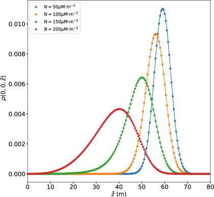
In the absence of nutrients, $\beta_{D}=0$ , Figure 2 shows how the distribution of bio-particles parallel to the temperature gradient (the $\tilde{z}$ -axis) is influenced by EPS/AFP production, which is modeled as a surface colligative effect. Namely, with $N_{i}=50\mu$ M m^-2 and four biological enhancement factors $n\in\{1,2,3,4\}$ . The active diffusivity is $\tilde{D}_{a}=100\tilde{D}$ and the particle radius is $R=9.0\times 10^{-6}$ m.

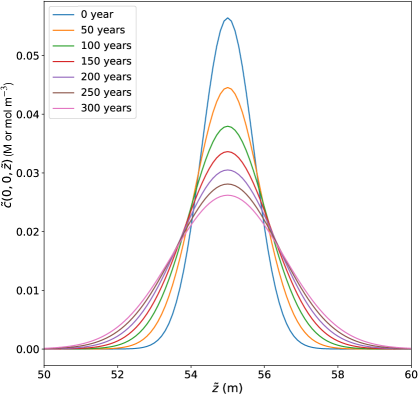
Figure 3 shows the evolution of the nutrient concentration along the $\tilde{z}$ -axis computed from Eq. (33), at $\tilde{x}=\tilde{y}=0$ . The nutrients are centered at $\tilde{z}_{0}=55$ m at $\tilde{t}=0$ and we use a nutrient diffusivity of $\tilde{D}_{ch}=10^{-10}$ m²s^-1 [128, 129, 130, 131].
In order to study the effect of nutrients on bio-locomotion, we fix the interfacial concentration of impurities and vary the chemotaxis strength $\beta_{D}$ , where nutrients either attract ( $\beta_{D}>0$ ) or repel ( $\beta_{D}<0$ ) the bio-particles. Because we are interested in the situation wherein the effects of chemotaxis compete with regelation, this constrains the magnitude of $\beta_{D}$ as follows. We ask for what order of magnitude of $\beta_{D}$ are the typical chemotactic speeds approximately the same as the regelation velocity in Eq. (4). Figure 3 shows the Gaussian solution of the concentration field, with a flux that becomes arbitrarily small at long times, dominated by the algebraic contribution to $\nabla_{\tilde{\bm{r}}}\tilde{\mathcal{C}}(\tilde{\bm{r}},\tilde{t})\propto x{t^{-3/2}}\exp(-\frac{x^{2}}{t})\sim x{t^{-3/2}}$ . For the parameters studied here, the regelation speeds are $10^{-12}-10^{-10}$ m s^-1 [53, 95], and hence we capture this same range in $\beta_{D}\nabla_{\tilde{\bm{r}}}\tilde{\mathcal{C}}(\tilde{\bm{r}},\tilde{t})$ , with $|\beta_{D}|=10^{-10}$ m²M^-1s^-1, which is realized across a large time span wherein $\nabla_{\tilde{\bm{r}}}\tilde{\mathcal{C}}(\tilde{\bm{r}},\tilde{t})$ varies by several orders of magnitude. This is also reflected in the dimensionless ratio $\beta_{D}\frac{c_{h}}{D_{c}}$ in Eq. (13). Namely, for micron to nm scale premelted films surrounding micron sized particles ${D_{c}}$ ranges from about $10^{-14}-10^{-13}$ m²s^-1, and the nutrient concentration over relevant time scales has mean values ranging over $10^{-3}-10^{-2}$ M. Therefore, $\beta_{D}\frac{c_{h}}{D_{c}}$ ranges from 1 to 100 and hence chemotaxis is on a similar footing to regelation under these circumstances. For all cases considered here we use $\beta_{D}=\pm 10^{-10}$ m²M^-1s^-1 for attractive/repulsive chemotaxis.
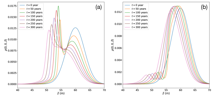
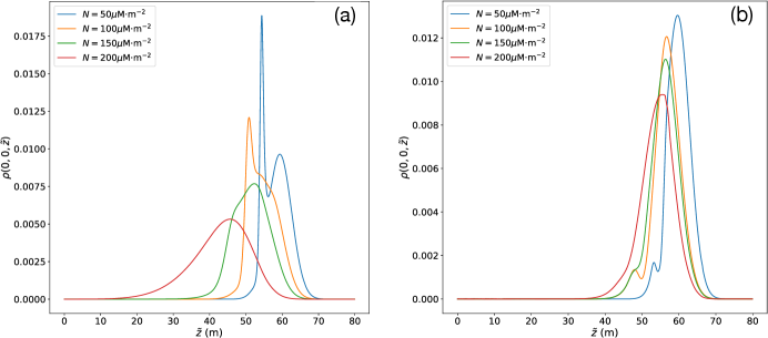
For attractive chemotaxis ( $\beta_{D}>0$ ), we show in Figure 4 (a) the dependence of $\rho(\bm{\tilde{r}},\tilde{t})$ along the $\tilde{z}$ -axis parallel to the temperature gradient and at $\tilde{x}=\tilde{y}=0$ , with the concentration of nutrients centered at $\tilde{z}=55$ m. For the same conditions in the absence of chemotaxis, the net displacement from low to high temperatures due to regelation is approximately 10 m [95]. We see here the chemo-attractive modulation of $\rho(\bm{\tilde{r}},\tilde{t})$ during this displacement, which “pulls up” the high temperature (low $\tilde{z}$ ) tail towards the lower temperature (large $\tilde{z}$ ) but higher concentration regions centered at $\tilde{z}=55$ m. The associated asymmetry depletes/attracts the low temperature regions at larger $\tilde{z}$ and concentrates the high temperature regions at smaller $\tilde{z}$ , and is reflected in the evolution towards a sigmoidal region transecting the source at $\tilde{z}=55$ m. As the maximum of $\rho(\bm{\tilde{r}},\tilde{t})$ advects through the source region it first sharpens, due to the chemo-attraction from the source “behind” it at $\tilde{z}=55$ m, and then begins to spread out again because of the decay in the chemotactic gradient in time as seen in Figure 3 and discussed above.
For repulsive chemotaxis ( $\beta_{D}<0$ ), we see in Figure 4 (b) the broad sharpening of the initial distribution in the lower temperature (large $\tilde{z}$ ) regions as it regelates/advects into the diffuse repulsive tail of nutrient field to the right of the source region centered at $\tilde{z}=55$ m. However, because the initial high temperature (small $\tilde{z}$ ) tail of $\rho(\bm{\tilde{r}},\tilde{t})$ interacts with the nutrient source region at $\tilde{z}=55$ m, chemo-repulsion quickly drives particles towards high temperature (small $\tilde{z}$ ) regions, and is clearly reflected in the creation of a local maximum. This maximum advects towards high temperature with a decaying amplitude and width due to the decay in the chemotactic gradient in time as seen in Figure 3.
In Fig. 5, we show the combined effects of EPS/AFP surface enhancement of impurities in the absence of chemotaxis ( $\beta_{D}=0$ ), as shown in Fig. 2, and the influence of chemotaxis on particle dynamics for fixed surface impurities, as shown in Fig. 4. As we vary the surface concentration of impurities we observe the same basic features as described in Figs. 2 and 4 and hence the same physical description applies in their interpretation. Namely, regardless of whether chemo-attraction or chemo-repulsion is operative, if the interfacial concentration of impurities $N$ is sufficiently large then the interfacial film thicknesses are sufficiently thick that thermal regelation dominates the evolution of $\rho(\bm{\tilde{r}},\tilde{t})$ . As the interfacial concentration of impurities $N$ decreases chemotaxis exerts more control on the distribution, and the basic dynamics are the same as described in Fig. 4. Because the magnitude of $\beta_{D}$ is fixed, and the characteristic concentration $c_{h}$ is $10^{-2}$ M, this $N$ -dependence is simply assessed as discussed above, in terms of the dimensionless ratio $\beta_{D}\frac{c_{h}}{D_{c}}$ in Eq. (13). Namely, the numerator is fixed, but as $N$ increases so too is the film thickness $d$ through Eq. (1), and since ${D_{c}}\propto d^{3}$ [52], then $\beta_{D}\frac{c_{h}}{D_{c}}$ decreases as $N^{-3}$ , and the balance between chemotaxis control of the distribution gives way to regelation control. The corpus of effects studied here are reflected in this basic balance and shown in Figs. 2, 4 and 5.

IV Conclusion

Micro-organisms in ice exhibit complex processes to persist and evolve in their harsh environments. They have developed different survival strategies, such as producing exopolymeric substances or antifreeze glycoproteins, and directing their motion toward nutrients or away from waste [39, 132, 133, 74]. We have modeled such micro-organisms using active Ornstein-Uhlenbeck particles subject to thermal regelation and biolocomotion in three dimensions. Firstly, we used a multi-scale expansion to derive the relevant coupled Fokker-Planck and diffusion equations (32)-(33). Secondly, when nutrients are neglected, and the chemotactic strength $\beta_{D}=0$ , we model the bio-production of surface chemicals, such as exopolymeric substances or antifreeze glycoproteins, as a surface colligative effect, and find that the associated bio-enhanced thermal regelation can dominate the distribution of particles in ice. Consistent with previous results [95], in a large Péclet number limit analytical solutions for the particle distributions are possible, and are consistent with the numerical solutions as shown in Fig. 2. Thirdly, we studied the competition between thermal regelation and biolocomotion, as function of the chemotaxis strength $\beta_{D}$ , the interplay between which is shown in Figs. 4-5. The relative importance of chemo-attraction and chemo-repulsion to thermal regelation is captured by the dimensionless ratio $\beta_{D}\frac{c_{h}}{D_{c}}$ . When this ratio is large we find a complex modulation of regelation by chemotaxis, and when small, due to increased surface impurity concentration, leads to regelation dominated redistribution of particles. We note, however, that we have not treated the process wherein nutrients themselves have a colligative effect, which would introduce a particularly complex spatio-temporal dynamics.

Finally, we describe settings to which our analysis is applicable. It is of general interest to understand how particles in ice migrate in response to environmental forcing, as they are used as proxy to infer past climate [134, 19, 135]. Moreover, bioparticles in ice migrate in response to environmental forcing, and micro-organisms play an important role in climate change [136, 137, 138]. For example, an increase in temperature activates algae/bacteria trapped in ice, producing chemicals that increase their mobility [138]. Indeed, an increase in algae/bacteria decreases the albedo of the ice [139, 140, 141], thereby enhancing melting. Finally, understanding the distribution and viability of bioparticles in partially frozen media on Earth [e.g., 142, 143] is essential in astrobiology [144, 145, 47].

Conflict of Interest Statement

The authors declare no competing interests.

Author Contributions

J.S.W. conceived the project. J.V. implemented the theory and performed simulations. J.S.W. and J.V. interpreted the data and wrote the paper. All authors contributed to the discussions and the final version of the manuscript.

Funding

This work was supported by the Swedish Research Council grant no. 638-2013-9243. Nordita is partially supported by Nordforsk.

Acknowledgments

We thank Matthias Geilhufe, Navaneeth Marath and István Mátá Szécsényi for helpful conversations.

V Appendix

V.1 Multiple scales Analysis

The solution of the leading order Eq. (29) is derived by making the following product ansatz

P^{0}(\bm{r},\bm{R},\bm{\eta},T,t)=w(\bm{r},\bm{\eta})\rho^{0}(\bm{R},T,t)\,.

(34)

Integrating by parts over the microscale variables $\bm{r}$ and $\bm{\eta}$ , and using the solvability condition, the solution of Eq. (29) $P^{0}$ is constant over the period: $P^{0}(\bm{r},\bm{R},\bm{\eta},T,t)=P^{0}(\bm{R},\bm{\eta},T,t)$ . The leading order Eq. (29) becomes

\nabla_{\bm{\eta}}\cdot\left[\bm{\eta}w\right]+\frac{1}{2}\nabla^{2}_{\bm{\eta}}w=0\,.

(35)

Using the known result for a multi-dimensional Ornstein-Uhlenbeck process [146], the solution for $w$ is given by

w(\eta_{1},\eta_{2},\eta_{3})=\prod\limits_{i=1}^{3}\frac{1}{\sqrt{2\pi}}e^{\dfrac{-\eta^{2}_{i}}{2}}\,.

(36)

The solvability condition for $\mathcal{O}(\epsilon)$ equation is

\displaystyle\int d\bm{r}d\bm{\eta}

\displaystyle\left(w\frac{\partial}{\partial T}\rho^{0}+w\frac{\partial}{\partial R_{3}}\left[v\rho^{0}\right]+wP_{a}v_{a}\bm{\eta}\cdot\nabla_{\bm{R}}\rho^{0}\right)=0\,,

(37)

which depends on the leading order result, $P^{0}$ , from which we find

\frac{\partial}{\partial T}\rho^{0}=-\frac{\partial}{\partial R_{3}}\left[v\rho^{0}\right]\,,

(38)

and the $\mathcal{O}(\epsilon)$ equation becomes

\mathcal{L}P^{1}=wP_{a}v_{a}\bm{\eta}\cdot\nabla_{\bm{R}}\rho^{0}\,.

(39)

We assume that

P^{1}=wP_{a}v_{a}\bm{\alpha}\cdot\nabla_{\bm{R}}\rho^{0}\,,

(40)

after which we find that

\bm{\alpha}=-\frac{1}{P_{A}}\bm{\eta}\,.

(41)

Substitution of $P^{1}$ into the $\mathcal{O}(\epsilon^{2})$ equation and using the solvability condition, we obtain

\frac{\partial}{\partial t}\rho^{0}=\frac{P_{a}^{2}v_{a}^{2}}{2P_{A}}\nabla^{2}_{\bm{R}}\rho^{0}-\beta_{D}\frac{c_{h}}{D_{c}}\nabla_{\bm{R}}\cdot\left[\rho^{0}\nabla_{\bm{R}}c^{0}\right]+\nabla_{\bm{R}}^{2}\left[D\rho^{0}\right]\,,

(42)

and in dimensional form, we have

\frac{\partial}{\partial\tilde{t}}\rho=-\beta_{D}\nabla_{\tilde{\bm{r}}}\cdot\left[\rho\nabla_{\tilde{\bm{r}}}\tilde{c}\right]-\frac{\partial}{\partial\tilde{z}}\left[\tilde{v}\rho\right]+\nabla^{2}_{\tilde{\bm{r}}}\left[(\tilde{D}_{a}+\tilde{D})\rho\right]\,.

(43)

V.2 Solution of the Fokker-Planck equation in the large Péclet limit

The analytic solution of Eq. (32) in the large Péclet number limit follows by expanding the probability density function, $\rho$ perturbatively [147], as

\rho=\rho_{0}+\rho_{1}\,,

(44)

with $\rho_{1}=\mathcal{O}(\tilde{c})\rho_{0}$ . The associated system of equations is

	$\displaystyle\frac{\partial}{\partial\tilde{t}}\rho_{0}+\frac{\partial}{\partial\tilde{z}}\left[\tilde{v}\rho_{0}\right]-\nabla^{2}_{\tilde{r}}\left[(\tilde{D}_{a}+\tilde{D})\rho_{0}\right]$	$\displaystyle=0\,,$		(45)
	$\displaystyle\frac{\partial}{\partial\tilde{t}}\rho_{1}+\frac{\partial}{\partial\tilde{z}}\left[\tilde{v}\rho_{1}\right]-\nabla^{2}_{\tilde{r}}\left[(\tilde{D}_{a}+\tilde{D})\rho_{1}\right]$	$\displaystyle=-\beta_{D}\nabla_{\tilde{\bm{r}}}\cdot\left[\rho_{0}\nabla_{\tilde{\bm{r}}}\tilde{c}\right]\,.$		(46)

To derive the solutions for $\rho_{0}$ and $\rho_{1}$ , we use the Green’s function $G(\tilde{\bm{r}},\tilde{t}|\tilde{\bm{r}_{0}},\tilde{t}_{0})$ [148] which satisfies

\frac{\partial}{\partial\tilde{t}}G+\frac{\partial}{\partial\tilde{z}}\left[\tilde{v}G\right]-\nabla^{2}_{\tilde{\bm{r}}}\left[(\tilde{D}_{a}+\tilde{D})G\right]=0\,.

(47)

The solution of Eq.(47) was derived in the large Péclet number limit in [95], and is

	$\displaystyle\rho_{0}=G(\tilde{\bm{r}},\tilde{t}\|\tilde{\bm{r}_{0}},\tilde{t}_{0})$	$\displaystyle=\frac{\tilde{z}^{3}}{(\tilde{z}^{\prime})^{3/4}}\exp\left(-\frac{\left[(\tilde{z}^{\prime})^{1/4}-\tilde{z}_{0}\right]^{2}}{20+4\tilde{D}_{a}(\tilde{t}-\tilde{t}_{0})}\right)\exp\left[-\frac{((\tilde{x}-\tilde{x}_{0})^{2}+(\tilde{y}-\tilde{y}_{0})^{2})}{\left(1+4\frac{\tilde{D}(\tilde{z})}{\tilde{v}(\tilde{z})}\left[(\tilde{z}^{\prime})^{1/4}-\tilde{z}\right]+4\tilde{D}_{a}(\tilde{t}-\tilde{t}_{0})\right)}\right]$
		$\displaystyle\times\frac{1}{2\sqrt{5\pi}\left(1+4\frac{\tilde{D}(\tilde{z})}{\tilde{v}(\tilde{z})}\left[(\tilde{z}^{\prime})^{1/4}-\tilde{z}\right]+4\tilde{D}_{a}(\tilde{t}-\tilde{t}_{0})\right)}\,.$		(48)

Given the Green’s function the formal solution of Eq.(32) is

\displaystyle\rho(\tilde{\bm{r}},\tilde{t})

\displaystyle=G(\tilde{\bm{r}},\tilde{t}|\tilde{\bm{r}_{0}},\tilde{t}_{0})-\beta_{D}\int\limits_{\tilde{t}_{0}}^{\tilde{t}}d\tau\int\limits d\tilde{\bm{r}}_{1}G(\tilde{\bm{r}},\tilde{t},|\tilde{\bm{r}}_{1},\tau)\left[\nabla_{\tilde{\bm{r}}_{1}}\left(G(\tilde{\bm{r}}_{1},\tau|\tilde{\bm{r}}_{0},\tilde{t}_{0})\nabla_{\tilde{\bm{r}}_{1}}\tilde{c}(\tilde{\bm{r}}_{1},\tau|\tilde{\bm{r}}_{0},\tilde{t}_{0})\right)\right]\,,

(49)

with

\tilde{c}(\tilde{\bm{r}},\tilde{t}|\tilde{\bm{r}}_{0},\tilde{t}_{0})=\frac{1}{\left(4\pi\tilde{D}_{ch}(\tilde{t}-\tilde{t}_{0})\right)^{\frac{3}{2}}}\exp\left[-\frac{((\tilde{x}-\tilde{x}_{0})^{2}+(\tilde{y}-\tilde{y}_{0})^{2}+(\tilde{z}-\tilde{z}_{0})^{2})}{4\tilde{D}_{ch}(\tilde{t}-\tilde{t}_{0})}\right]\,.

(50)

At $\tilde{t}_{0}=0$ and $\tilde{x}_{0}=\tilde{y}_{0}=0$ , the initial distribution is, to leading order $\rho_{0}$ , given by

\rho_{0}(\tilde{\bm{r}},\tilde{t}=0)=\frac{1}{2\sqrt{5\pi}}\exp\left[-\frac{(\tilde{z}-\tilde{z}_{0})^{2}}{20}-(\tilde{x}^{2}+\tilde{y}^{2})\right]\,.

(51)

Equations (49) and (50) give the analytic solution to Eqs. (32)-(33), with initial distribution given by Eq. (51). When the nutrients are neglected we recover our previous result [95].

References

Karl et al. [1999] D. Karl, D. Bird, K. Björkman, T. Houlihan, R. Shackelford, and L. Tupas, Microorganisms in the accreted ice of Lake Vostok, Antarctica, Science 286, 2144 (1999).
Christner et al. [2001] B. Christner, E. Mosley-Thompson, L. Thompson, and J. Reeve, Isolation of bacteria and 16s rDNAs from Lake Vostok accretion ice, Environ. Microbiol. 3, 570 (2001).
Anesio et al. [2007] A. M. Anesio, B. Mindl, J. Laybourn-Parry, A. J. Hodson, and B. Sattler, Viral dynamics in cryoconite holes on a high Arctic glacier (Svalbard), J. Geophys. Res-Biogeo. 112 (2007).
Bellas et al. [2015] C. M. Bellas, A. M. Anesio, and G. Barker, Analysis of virus genomes from glacial environments reveals novel virus groups with unusual host interactions, Front. Microbiol. 6, 656 (2015).
Heilmann et al. [2012] S. Heilmann, K. Sneppen, and S. Krishna, Coexistence of phage and bacteria on the boundary of self-organized refuges, Proc. Natl. Acad. Sci. - USA 109, 12828 (2012).
Zhong et al. [2021a] Z.-P. Zhong, F. Tian, S. Roux, M. C. Gazitúa, N. E. Solonenko, Y.-F. Li, M. E. Davis, J. L. Van Etten, E. Mosley-Thompson, V. I. Rich, et al., Glacier ice archives nearly 15,000-year-old microbes and phages, Microbiome 9, 1 (2021a).
Yau et al. [2011] S. Yau, F. M. Lauro, M. Z. DeMaere, M. V. Brown, T. Thomas, M. J. Raftery, C. Andrews-Pfannkoch, M. Lewis, J. M. Hoffman, J. A. Gibson, et al., Virophage control of antarctic algal host–virus dynamics, Proc. Natl. Acad. Sci. - USA 108, 6163 (2011).
Legendre et al. [2014] M. Legendre, J. Bartoli, L. Shmakova, S. Jeudy, K. Labadie, A. Adrait, M. Lescot, O. Poirot, L. Bertaux, C. Bruley, et al., Thirty-thousand-year-old distant relative of giant icosahedral DNA viruses with a pandoravirus morphology, P. Natl. Acad. Sci. USA 111, 4274 (2014).
Zhong et al. [2021b] Z.-P. Zhong, F. Tian, S. Roux, M. C. Gazitúa, N. E. Solonenko, Y.-F. Li, M. E. Davis, J. L. Van Etten, E. Mosley-Thompson, V. I. Rich, et al., Glacier ice archives nearly 15,000-year-old microbes and phages, Microbiome 9, 1 (2021b).
El-Sayed and Kamel [2021] A. El-Sayed and M. Kamel, Future threat from the past, Environ. Sci. Pollut. R. 28, 1287 (2021).
Shatilovich et al. [2018] A. Shatilovich, A. Tchesunov, T. Neretina, I. Grabarnik, S. Gubin, T. Vishnivetskaya, T. Onstott, and E. Rivkina, Viable nematodes from late pleistocene permafrost of the kolyma river lowland, in Doklady Biological Sciences, Vol. 480 (Springer, 2018) pp. 100–102.
Christner et al. [2003] B. Christner, E. Mosley-Thompson, L. Thompson, and J. Reeve, Bacterial recovery from ancient glacial ice, Environ. Microbiol. 5, 433 (2003).
Doyle and Christner [2021] S. Doyle and B. Christner, Microbial composition, diversity, and activity varies across different types of basal ice, bioRxiv (2021).
Anesio et al. [2017] A. M. Anesio, S. Lutz, N. A. M. Chrismas, and L. G. Benning, The microbiome of glaciers and ice sheets, npj Biofilms and Microbiomes 3, 1 (2017).
Royer et al. [1983] A. Royer, M. De Angelis, and J. R. Petit, A 30000 year record of physical and optical properties of microparticles from an East Antarctic ice core and implications for paleoclimate reconstruction models, Climatic Change 5, 381 (1983).
Legrand and Mayewski [1997] M. Legrand and P. Mayewski, Glaciochemistry of polar ice cores: A review, Rev. Geophys. 35, 219 (1997).
Stauffer et al. [2004] B. Stauffer, J. Flückiger, E. Wolff, and P. Barnes, The EPICA deep ice cores: first results and perspectives, Ann. Glaciol. 39, 93 (2004).
Alley [2010] R. B. Alley, Reliability of ice-core science: historical insights, J. Glaciol. 56, 1095 (2010).
Thomas et al. [2015] C. Thomas, D. Ionescu, D. Ariztegui, and D. S. Team, Impact of paleoclimate on the distribution of microbial communities in the subsurface sediment of the dead sea, Geobiology 13, 546 (2015).
Tetzner et al. [2021] D. Tetzner, E. R. Thomas, C. S. Allen, and E. W. Wolff, A refined method to analyze insoluble particulate matter in ice cores, and its application to diatom sampling in the Antarctic Peninsula, Front. Earth Sci. 9, 20 (2021).
Papina et al. [2013] T. Papina, T. Blyakharchuk, A. Eichler, N. Malygina, E. Mitrofanova, and M. Schwikowski, Biological proxies recorded in a Belukha ice core, Russian Altai, Clim. Past 9, 2399 (2013).
Mao et al. [2022] G. Mao, M. Ji, B. Xu, Y. Liu, and N. Jiao, Variation of high (HNA) and low (LNA) nucleic acid-content bacteria in Tibetan ice cores and their relationship to black carbon, Front. Microbiol. , 299 (2022).
Achberger et al. [2011] A. M. Achberger, T. I. Brox, M. L. Skidmore, and B. C. Christner, Expression and characterization of an ice binding protein from a bacterium isolated at a depth of 3,519 meters in the Vostok ice core, Antarctica, Front. Microbiol. 2, 255 (2011).
Knowlton et al. [2013] C. Knowlton, R. Veerapaneni, T. D’Elia, and S. O. Rogers, Microbial analyses of ancient ice core sections from Greenland and Antarctica, Biology 2, 206 (2013).
Garcia-Lopez et al. [2021a] E. Garcia-Lopez, A. Moreno, M. Bartolomé, M. Leunda Esnaola, C. Sancho, and C. Cid, Glacial Ice Age Shapes Microbiome Composition in a Receding Southern European Glacier, Front. Microbiol. 12 (2021a).
Wilhelm et al. [2013] L. Wilhelm, G. A. Singer, C. Fasching, T. J. Battin, and K. Besemer, Microbial biodiversity in glacier-fed streams, The ISME journal 7, 1651 (2013).
Garcia-Lopez et al. [2021b] E. Garcia-Lopez, A. Moreno, M. Bartolomé, M. Leunda Esnaola, C. Sancho, and C. Cid, Glacial ice age shapes microbiome composition in a receding southern european glacier, Front. Mar. Sci. 12 (2021b).
Stibal et al. [2015] M. Stibal, M. Schostag, K. A. Cameron, L. H. Hansen, D. M. Chandler, J. L. Wadham, and C. S. Jacobsen, Different bulk and active bacterial communities in cryoconite from the margin and interior of the Greenland ice sheet, Env. Microbiol. Rep. 7, 293 (2015).
Hop et al. [2020] H. Hop, M. Vihtakari, B. A. Bluhm, P. Assmy, M. Poulin, R. Gradinger, I. Peeken, C. von Quillfeldt, L. M. Olsen, L. Zhitina, et al., Changes in sea-ice protist diversity with declining sea ice in the Arctic Ocean from the 1980s to 2010s, Front. Mar. Sci. 7, 243 (2020).
Kauko et al. [2018] H. M. Kauko, L. M. Olsen, P. Duarte, I. Peeken, M. A. Granskog, G. Johnsen, M. Fernández-Méndez, A. K. Pavlov, C. J. Mundy, and P. Assmy, Algal colonization of young Arctic sea ice in spring, Front. Mar. Sci. 5, 199 (2018).
Spilling et al. [2018] K. Spilling, K. Olli, J. Lehtoranta, A. Kremp, L. Tedesco, T. Tamelander, R. Klais, H. Peltonen, and T. Tamminen, Shifting diatom—dinoflagellate dominance during spring bloom in the Baltic Sea and its potential effects on biogeochemical cycling, Front. Mar. Sci. 5, 327 (2018).
Itcus et al. [2018] C. Itcus, M. D. Pascu, P. Lavin, A. Perşoiu, L. Iancu, and C. Purcarea, Bacterial and archaeal community structures in perennial cave ice, Sci. Rep. 8, 1 (2018).
Miyata et al. [2020] M. Miyata, R. C. Robinson, T. Q. Uyeda, Y. Fukumori, S.-i. Fukushima, S. Haruta, M. Homma, K. Inaba, M. Ito, C. Kaito, et al., Tree of motility–A proposed history of motility systems in the tree of life, Genes Cells 25, 6 (2020).
Hahnke et al. [2016] R. L. Hahnke, J. P. Meier-Kolthoff, M. García-López, S. Mukherjee, M. Huntemann, N. N. Ivanova, T. Woyke, N. C. Kyrpides, H.-P. Klenk, and M. Göker, Genome-based taxonomic classification of Bacteroidetes, Front. Microbiol. 7, 2003 (2016).
Hill and Häder [1997] N. Hill and D.-P. Häder, A biased random walk model for the trajectories of swimming micro-organisms, J. Theor. Biol. 186, 503 (1997).
Tsagkari and Sloan [2018] E. Tsagkari and W. T. Sloan, The role of the motility of methylobacterium in bacterial interactions in drinking water, Water 10, 1386 (2018).
Doerges and Kutschera [2014] L. Doerges and U. Kutschera, Assembly and loss of the polar flagellum in plant-associated methylobacteria, Naturwissenschaften 101, 339 (2014).
Svensson et al. [2014] F. Svensson, J. Norberg, and P. Snoeijs, Diatom cell size, coloniality and motility: trade-offs between temperature, salinity and nutrient supply with climate change, PloS one 9, e109993 (2014).
Aumack et al. [2014] C. F. Aumack, A. R. Juhl, and C. Krembs, Diatom vertical migration within land-fast Arctic sea ice, J. Marine Syst. 139, 496 (2014).
Christner et al. [2000] B. C. Christner, E. Mosley-Thompson, L. G. Thompson, V. Zagorodnov, K. Sandman, and J. N. Reeve, Recovery and identification of viable bacteria immured in glacial ice, Icarus 144, 479 (2000).
Biswas and Choudhury [2021] R. K. Biswas and A. K. Choudhury, Diatoms: Miniscule biological entities with immense importance in synthesis of targeted novel bioparticles and biomonitoring, J. Biosciences 46, 1 (2021).
Dong et al. [2010] H. Dong, H. Jiang, B. Yu, X. Liu, C. Zhang, and M. Chan, Impacts of environmental change and human activity on microbial ecosystems on the Tibetan Plateau, NW China, Gsa Today 20, 4 (2010).
Delgado-Baquerizo et al. [2017] M. Delgado-Baquerizo, A. Bissett, D. J. Eldridge, F. T. Maestre, J.-Z. He, J.-T. Wang, K. Hamonts, Y.-R. Liu, B. K. Singh, and N. Fierer, Palaeoclimate explains a unique proportion of the global variation in soil bacterial communities, Nat. Ecol. Evol. 1, 1339 (2017).
Benningfield [2022] D. Benningfield, The bumpy search for liquid water at the South Pole of Mars, EOS 103, https://doi.org/10.1029/2022EO220126. (2022).
Lindensmith et al. [2016] C. A. Lindensmith, S. Rider, M. Bedrossian, J. K. Wallace, E. Serabyn, G. M. Showalter, J. W. Deming, and J. L. Nadeau, A submersible, off-axis holographic microscope for detection of microbial motility and morphology in aqueous and icy environments, PloS one 11, e0147700 (2016).
Nadeau et al. [2016a] J. Nadeau, C. Lindensmith, J. W. Deming, V. I. Fernandez, and R. Stocker, Microbial morphology and motility as biosignatures for outer planet missions, Astrobiology 16, 755 (2016a).
Jones et al. [2018] R. M. Jones, J. M. Goordial, and B. N. Orcutt, Low energy subsurface environments as extraterrestrial analogs, Front. Microbiol. 9, 1605 (2018).
Schreder-Gomes et al. [2022] S. I. Schreder-Gomes, K. C. Benison, and J. A. Bernau, 830-million-year-old microorganisms in primary fluid inclusions in halite, Geology (in press) https://doi.org/10.1130/G49957.1 (2022).
Dash et al. [2006] J. G. Dash, A. W. Rempel, and J. S. Wettlaufer, The physics of premelted ice and its geophysical consequences, Rev. Mod. Phys. 78, 695 (2006).
Rempel et al. [2001a] A. W. Rempel, J. S. Wettlaufer, and M. G. Worster, Interfacial premelting and the thermomolecular force: thermodynamic buoyancy, Phys. Rev. Lett. 87, 088501 (2001a).
Wettlaufer and Worster [2006] J. S. Wettlaufer and M. G. Worster, Premelting dynamics, Ann. Rev. Fluid Mech. 38, 427 (2006).
Peppin et al. [2009] S. S. L. Peppin, M. J. Spannuth, and J. S. Wettlaufer, Onsager reciprocity in premelting solids, J. Stat. Phys. 134, 701 (2009).
Marath and Wettlaufer [2020] N. K. Marath and J. S. Wettlaufer, Impurity effects in thermal regelation, Soft Matter 16, 5886 (2020).
Wingender et al. [1999] J. Wingender, T. Neu, and H.-C. Flemming, What are bacterial extracellular polymeric substances?, in Microbial extracellular polymeric substances (Springer, 1999) pp. 1–19.
Bang et al. [2013] J. Bang, J. Lee, R. Murugan, S. Lee, H. Do, H. Koh, H.-E. Shim, H.-C. Kim, and H. Kim, Antifreeze peptides and glycopeptides, and their derivatives: potential uses in biotechnology, Marine drugs 11 (2013).
Eskandari et al. [2020] A. Eskandari, T. Leow, M. Rahman, and S. Oslan, Antifreeze Proteins and Their Practical Utilization in Industry, Medicine, and Agriculture, Biomolecules 10, 1649 (2020).
Ewert and Deming [2014] M. Ewert and J. Deming, Bacterial responses to fluctuations and extremes in temperature and brine salinity at the surface of Arctic winter sea ice, FEMS Microbiol. Ecol. 89, 476 (2014).
Ewert and Deming [2013a] M. Ewert and J. Deming, Sea ice microorganisms: Environmental constraints and extracellular responses, Biology 2, 603 (2013a).
Krembs et al. [2011] C. Krembs, H. Eicken, and J. W. Deming, Exopolymer alteration of physical properties of sea ice and implications for ice habitability and biogeochemistry in a warmer Arctic, Proc. Nat. Acad. Sci. USA 108, 3653 (2011).
Decho and Gutierrez [2017] A. W. Decho and T. Gutierrez, Microbial extracellular polymeric substances (EPSs) in ocean systems, Front. Microbiol. 8, 922 (2017).
Cates [2012] M. E. Cates, Diffusive transport without detailed balance in motile bacteria: does microbiology need statistical physics?, Rep. Prog. Phys. 75, 042601 (2012).
Bechinger et al. [2016] C. Bechinger, R. Di Leonardo, H. Löwen, C. Reichhardt, G. Volpe, and G. Volpe, Active particles in complex and crowded environments, Rev. Mod. Phys. 88, 045006 (2016).
Ghosh and Fischer [2009] A. Ghosh and P. Fischer, Controlled propulsion of artificial magnetic nanostructured propellers, Nano Lett. 9, 2243 (2009).
Kim et al. [2013] S. Kim, F. Qiu, S. Kim, A. Ghanbari, C. Moon, L. Zhang, B. J. Nelson, and H. Choi, Fabrication and characterization of magnetic microrobots for three-dimensional cell culture and targeted transportation, Adv. Mat. 25, 5863 (2013).
Jin et al. [2019] C. Jin, J. Vachier, S. Bandyopadhyay, T. Macharashvili, and C. C. Maass, Fine balance of chemotactic and hydrodynamic torques: When microswimmers orbit a pillar just once, Phys. Rev. E 100, 040601 (2019).
Elgeti et al. [2015] J. Elgeti, R. G. Winkler, and G. Gompper, Physics of microswimmers–single particle motion and collective behavior: A review, Rep. Prog. Phys. 78, 056601 (2015).
Romanczuk et al. [2012] P. Romanczuk, M. Bär, W. Ebeling, B. Lindner, and L. Schimansky-Geier, Active Brownian particles, Eur. Phys. J.-Spec. Top. 202, 1 (2012).
Li and Tian [2012] Y.-H. Li and X. Tian, Quorum sensing and bacterial social interactions in biofilms, Sensors 12, 2519 (2012).
Yan and Wu [2019] S. Yan and G. Wu, Can biofilm be reversed through quorum sensing in Pseudomonas aeruginosa?, Front. Microbiol. 10, 1582 (2019).
Lee et al. [2020] C. K. Lee, J. Vachier, J. de Anda, K. Zhao, A. E. Baker, R. R. Bennett, C. R. Armbruster, K. A. Lewis, R. L. Tarnopol, C. J. Lomba, et al., Social cooperativity of bacteria during reversible surface attachment in young biofilms: a quantitative comparison of Pseudomonas aeruginosa PA14 and PAO1, MBio 11, e02644 (2020).
Wadhams and Armitage [2004] G. H. Wadhams and J. P. Armitage, Making sense of it all: bacterial chemotaxis, Nat. Rev. Mol. Cell Bio. 5, 1024 (2004).
Showalter and Deming [2018a] G. Showalter and J. Deming, Low-temperature chemotaxis, halotaxis and chemohalotaxis by the psychrophilic marine bacterium colwellia psychrerythraea 34h, Env. Microbiol. Rep. 10, 92 (2018a).
Cremer et al. [2019] J. Cremer, T. Honda, Y. Tang, J. Wong-Ng, M. Vergassola, and T. Hwa, Chemotaxis as a navigation strategy to boost range expansion, Nature 575, 658 (2019).
Bar Dolev et al. [2016] M. Bar Dolev, R. Bernheim, S. Guo, P. L. Davies, and I. Braslavsky, Putting life on ice: bacteria that bind to frozen water, J. R. Soc. Interface 13, 20160210 (2016).
Mattingly et al. [2021] H. Mattingly, K. Kamino, B. Machta, and T. Emonet, Escherichia coli chemotaxis is information limited, Nat. Phys. , 1 (2021).
Bar-Dolev et al. [2012] M. Bar-Dolev, Y. Celik, J. S. Wettlaufer, P. L. Davies, and I. Braslavsky, New insights into ice growth and melting modifications by antifreeze proteins, J. R. Soc. Interface 9, 3249 (2012).
Hansen-Goos et al. [2014] H. Hansen-Goos, E. S. Thomson, and J. S. Wettlaufer, On the edge of habitability and the extremes of liquidity, Planet. Space Sci. 98, 169 (2014).
Showalter and Deming [2018b] G. Showalter and J. Deming, Low-temperature chemotaxis, halotaxis and chemohalotaxis by the psychrophilic marine bacterium Colwellia psychrerythraea 34H, Env. Microbiol. Reports 10, 92 (2018b).
Junge et al. [2003] K. Junge, H. Eicken, and J. W. Deming, Motility of Colwellia psychrerythraea strain 34H at subzero temperatures, Appl. Environ. Microb. 69, 4282 (2003).
Mudge et al. [2021] M. C. Mudge, B. L. Nunn, E. Firth, M. Ewert, K. Hales, W. E. Fondrie, W. S. Noble, J. Toner, B. Light, and K. A. Junge, Subzero, saline incubations of Colwellia psychrerythraea reveal strategies and biomarkers for sustained life in extreme icy environments, Environ. Microbiol. 23, 3840 (2021).
Wadham et al. [2019] J. L. Wadham, J. R. Hawkings, L. Tarasov, L. J. Gregoire, R. G. M. Spencer, M. Gutjahr, A. Ridgwell, and K. E. Kohfeld, Ice sheets matter for the global carbon cycle, Nat. Commun. 10, 1 (2019).
Holland et al. [2019] A. T. Holland, C. J. Williamson, F. Sgouridis, A. J. Tedstone, J. McCutcheon, J. M. Cook, E. Poniecka, M. L. Yallop, M. Tranter, A. M. Anesio, et al., Dissolved organic nutrients dominate melting surface ice of the Dark Zone (Greenland Ice Sheet), Biogeosciences 16, 3283 (2019).
Fodor et al. [2016] É. Fodor, C. Nardini, M. E. Cates, J. Tailleur, P. Visco, and F. van Wijland, How far from equilibrium is active matter?, Phys. Rev. Lett. 117, 038103 (2016).
Caprini and Marconi [2018] L. Caprini and U. M. B. Marconi, Active particles under confinement and effective force generation among surfaces, Soft Matter 14, 9044 (2018).
Martin et al. [2021] D. Martin, J. O’Byrne, M. E. Cates, É. Fodor, C. Nardini, J. Tailleur, and F. van Wijland, Statistical mechanics of active Ornstein-Uhlenbeck particles, Phys. Rev. E 103, 032607 (2021).
Dabelow and Eichhorn [2021] L. Dabelow and R. Eichhorn, Irreversibility in Active Matter: General Framework for Active Ornstein-Uhlenbeck Particles, Front. Phys. 8, 516 (2021).
Caprini et al. [2019] L. Caprini, U. M. B. Marconi, and A. Puglisi, Activity induced delocalization and freezing in self-propelled systems, Sci. Rep. 9, 1 (2019).
Bonilla [2019] L. L. Bonilla, Active Ornstein-Uhlenbeck particles, Phys. Rev. E 100, 022601 (2019).
Dabelow et al. [2019] L. Dabelow, S. Bo, and R. Eichhorn, Irreversibility in Active Matter Systems: Fluctuation Theorem and Mutual Information, Phys. Rev. X 9, 021009 (2019).
Sevilla et al. [2019] F. J. Sevilla, R. F. Rodríguez, and J. R. Gomez-Solano, Generalized Ornstein-Uhlenbeck model for active motion, Phys. Rev. E 100, 032123 (2019).
Maggi et al. [2014] C. Maggi, M. Paoluzzi, N. Pellicciotta, A. Lepore, L. Angelani, and R. Di Leonardo, Generalized energy equipartition in harmonic oscillators driven by active baths, Phys. Rev. Lett. 113, 238303 (2014).
Maggi et al. [2017] C. Maggi, M. Paoluzzi, L. Angelani, and R. Di Leonardo, Memory-less response and violation of the fluctuation-dissipation theorem in colloids suspended in an active bath, Sci. Rep. 7, 1 (2017).
Donado et al. [2017] F. Donado, R. E. Moctezuma, L. López-Flores, M. Medina-Noyola, and J. L. Arauz-Lara, Brownian motion in non-equilibrium systems and the Ornstein-Uhlenbeck stochastic process, Sci. Rep. 7, 1 (2017).
Marconi et al. [2016] U. M. B. Marconi, C. Maggi, and S. Melchionna, Pressure and surface tension of an active simple liquid: a comparison between kinetic, mechanical and free-energy based approaches, Soft Matter 12, 5727 (2016).
Vachier and Wettlaufer [2022] J. Vachier and J. S. Wettlaufer, Premelting controlled active matter in ice, Phys. Rev. E 105, 024601 (2022).
Wettlaufer [1999] J. S. Wettlaufer, Impurity effects in the premelting of ice, Phys. Rev. Lett. 82, 2516 (1999).
Ewert and Deming [2013b] M. Ewert and J. W. Deming, Sea ice microorganisms: Environmental constraints and extracellular responses, Biology 2, 603 (2013b).
Keller and Segel [1971] E. F. Keller and L. A. Segel, Model for chemotaxis, J. Theor. Biol. 30, 225 (1971).
Saha et al. [2014] S. Saha, R. Golestanian, and S. Ramaswamy, Clusters, asters, and collective oscillations in chemotactic colloids, Phys. Rev. E 89, 062316 (2014).
Liebchen and Löwen [2018a] B. Liebchen and H. Löwen, Synthetic chemotaxis and collective behavior in active matter, Accounts Chem. Res. 51, 2982 (2018a).
Pohl and Stark [2014] O. Pohl and H. Stark, Dynamic clustering and chemotactic collapse of self-phoretic active particles, Phys. Rev. Lett. 112, 238303 (2014).
Wettlaufer et al. [1997] J. S. Wettlaufer, M. G. Worster, and H. E. Huppert, Natural convection during solidification of an alloy from above with application to the evolution of sea ice, J. Fluid Mech. 344, 291 (1997).
Rempel et al. [2001b] A. W. Rempel, E. D. Waddington, J. S. Wettlaufer, and M. G. Worster, Possible displacement of the climate signal in ancient ice by premelting and anomalous diffusion, Nature 411, 568 (2001b).
Rempel et al. [2002] A. W. Rempel, J. S. Wettlaufer, and E. D. Waddington, Anomalous diffusion of multiple impurity species: Predicted implications for the ice core climate records, J. Geophys. Res.: Solid Earth 107, ECV 3 (2002).
Wells et al. [2010] A. J. Wells, J. S. Wettlaufer, and S. A. Orszag, Maximal potential energy transport: A variational principle for solidification problems, Phys. Rev. Lett. 105, 254502 (2010).
Joanny et al. [2003] J.-F. Joanny, F. Jülicher, and J. Prost, Motion of an adhesive gel in a swelling gradient: a mechanism for cell locomotion, Phys. Rev. Lett. 90, 168102 (2003).
Peruani and Morelli [2007] F. Peruani and L. G. Morelli, Self-propelled particles with fluctuating speed and direction of motion in two dimensions, Phys. Rev. Lett. 99, 010602 (2007).
Romanczuk and Schimansky-Geier [2011] P. Romanczuk and L. Schimansky-Geier, Brownian motion with active fluctuations, Phys. Rev. Lett. 106, 230601 (2011).
Vandebroek and Vanderzande [2017] H. Vandebroek and C. Vanderzande, The effect of active fluctuations on the dynamics of particles, motors and DNA-hairpins, Soft matter 13, 2181 (2017).
Price [2000] P. B. Price, A habitat for psychrophiles in deep Antarctic ice, Proc. Nat. Acad. Sci. USA 97, 1247 (2000).
Campen et al. [2003] R. K. Campen, T. Sowers, and R. B. Alley, Evidence of microbial consortia metabolizing within a low-latitude mountain glacier, Geology 31, 231 (2003).
Tung et al. [2006] H. Tung, P. Price, N. Bramall, and G. Vrdoljak, Microorganisms metabolizing on clay grains in 3-km-deep Greenland basal ice, Astrobiology 6, 69 (2006).
Mader et al. [2006] H. Mader, M. Pettitt, J. Wadham, E. Wolff, and R. Parkes, Subsurface ice as a microbial habitat, Geology 34, 169 (2006).
Rohde and Price [2007] R. A. Rohde and P. B. Price, Diffusion-controlled metabolism for long-term survival of single isolated microorganisms trapped within ice crystals, Proc. Nat. Acad. Sci. USA 104, 16592 (2007).
Vancoppenolle et al. [2010] M. Vancoppenolle, H. Goosse, A. De Montety, T. Fichefet, B. Tremblay, and J.-L. Tison, Modeling brine and nutrient dynamics in Antarctic sea ice: The case of dissolved silica, J. Geophys. Res-Oceans 115 (2010).
Wu et al. [2006] M. Wu, J. W. Roberts, S. Kim, D. L. Koch, and M. P. DeLisa, Collective bacterial dynamics revealed using a three-dimensional population-scale defocused particle tracking technique, Appl. Environ. Microb. 72, 4987 (2006).
Amar [2016] M. B. Amar, Collective chemotaxis and segregation of active bacterial colonies, Sci. Rep. 6, 1 (2016).
Wåhlin and Klein-Paste [2017] J. Wåhlin and A. Klein-Paste, The effect of mass diffusion on the rate of chemical ice melting using aqueous solutions, Cold Reg. Sci. Technol. 139, 11 (2017).
Liebchen and Löwen [2018b] B. Liebchen and H. Löwen, Synthetic chemotaxis and collective behavior in active matter, Accounts Chem. Res. 51, 2982 (2018b).
Dabelow et al. [2021] L. Dabelow, S. Bo, and R. Eichhorn, How irreversible are steady-state trajectories of a trapped active particle?, J. Stat. Mech.- Theory E. 2021, 033216 (2021).
Caprini et al. [2022] L. Caprini, U. M. B. Marconi, R. Wittmann, and H. Löwen, Dynamics of active particles with space-dependent swim velocity, Soft Matter (2022).
Bender and Orszag [2013] C. M. Bender and S. A. Orszag, Advanced Mathematical Methods for Scientists and Engineers: Asymptotic methods and perturbation theory (Springer Science & Business Media, 2013).
Pavliotis and Stuart [2008] G. Pavliotis and A. Stuart, Multiscale methods: averaging and homogenization (Springer Science & Business Media, 2008).
Aurell et al. [2016] E. Aurell, S. Bo, M. Dias, R. Eichhorn, and R. Marino, Diffusion of a Brownian ellipsoid in a force field, Europhys. Lett. 114, 30005 (2016).
Chipot [2009] M. Chipot, Elliptic Equations: An Introductory Course, in Elliptic Equations: An Introductory Course (Birkhäuser, Basel, Basel, 2009) Chap. Weak Formulation of Elliptic Problems, pp. 35–42.
Barenblatt [1996] G. I. Barenblatt, Scaling, Self-similarity, and Intermediate Asymptotics (Cambridge University Press, Cambridge, UK, 1996).
Liebchen and Löwen [2020] B. Liebchen and H. Löwen, Modeling Chemotaxis of Microswimmers: From Individual to Collective Behavior, in Chemical Kinetics: Beyond the Textbook (World Scientific, 2020) pp. 493–516.
Theurkauff et al. [2012] I. Theurkauff, C. Cottin-Bizonne, J. Palacci, C. Ybert, and L. Bocquet, Dynamic clustering in active colloidal suspensions with chemical signaling, Phys. Rev. Lett. 108, 268303 (2012).
Jin et al. [2017] C. Jin, C. Krüger, and C. C. Maass, Chemotaxis and autochemotaxis of self-propelling droplet swimmers, Proc. Nat. Acad. Sci. USA 114, 5089 (2017).
Salek et al. [2019] M. M. Salek, F. Carrara, V. Fernandez, J. S. Guasto, and R. Stocker, Bacterial chemotaxis in a microfluidic T-maze reveals strong phenotypic heterogeneity in chemotactic sensitivity, Nat. Commun. 10, 1 (2019).
Hokmabad et al. [2022] B. V. Hokmabad, S. Saha, J. Agudo-Canalejo, R. Golestanian, and C. C. Maass, Chemotactic self-caging in active emulsions, arXiv preprint arXiv:2012.05170 (2022).
Price [2007] P. B. Price, Microbial life in glacial ice and implications for a cold origin of life, FEMS Microbiol. Ecol. 59, 217 (2007).
Stocker and Seymour [2012] R. Stocker and J. R. Seymour, Ecology and physics of bacterial chemotaxis in the ocean, Microbiol. Mol. Biol. R. 76, 792 (2012).
Miteva [2008] V. Miteva, Bacteria in snow and glacier ice, in Psychrophiles: from biodiversity to biotechnology (Springer, 2008) pp. 31–50.
Han et al. [2017] D. Han, S.-I. Nam, J.-H. Kim, R. Stein, F. Niessen, Y. J. Joe, Y.-H. Park, and H.-G. Hur, Inference on paleoclimate change using microbial habitat preference in arctic holocene sediments, Sci. Rep. 7, 1 (2017).
Mitchell and Kogure [2006] J. G. Mitchell and K. Kogure, Bacterial motility: links to the environment and a driving force for microbial physics, FEMS Microbiol. Ecol. 55, 3 (2006).
Dutta and Dutta [2016] H. Dutta and A. Dutta, The microbial aspect of climate change, Energy, Ecol. Environ. 1, 209 (2016).
Cavicchioli et al. [2019] R. Cavicchioli, W. J. Ripple, K. N. Timmis, F. Azam, L. R. Bakken, M. Baylis, M. J. Behrenfeld, A. Boetius, P. W. Boyd, A. T. Classen, et al., Scientists’ warning to humanity: microorganisms and climate change, Nat. Rev. Microbiol. 17, 569 (2019).
Ryan et al. [2018] J. C. Ryan, A. Hubbard, M. Stibal, T. D. Irvine-Fynn, J. Cook, L. C. Smith, K. Cameron, and J. Box, Dark zone of the Greenland Ice Sheet controlled by distributed biologically-active impurities, Nat. Commun. 9, 1 (2018).
Perini et al. [2019] L. Perini, C. Gostinčar, A. M. Anesio, C. Williamson, M. Tranter, and N. Gunde-Cimerman, Darkening of the Greenland Ice Sheet: Fungal abundance and diversity are associated with algal bloom, Front. Microbiol. 10, 557 (2019).
Williamson et al. [2020] C. J. Williamson, J. Cook, A. Tedstone, M. Yallop, J. McCutcheon, E. Poniecka, D. Campbell, T. Irvine-Fynn, J. McQuaid, M. Tranter, et al., Algal photophysiology drives darkening and melt of the Greenland Ice Sheet, Proc. Natl. Acad. Sci. USA 117, 5694 (2020).
Van Leeuwe et al. [2018] M. A. Van Leeuwe, L. Tedesco, K. R. Arrigo, P. Assmy, K. Campbell, K. M. Meiners, J.-M. Rintala, V. Selz, D. N. Thomas, and J. Stefels, Microalgal community structure and primary production in arctic and antarctic sea ice: A synthesis, Elementa: Science of the Anthropocene 6 (2018).
Cimoli et al. [2020] E. Cimoli, V. Lucieer, K. M. Meiners, A. Chennu, K. Castrisios, K. G. Ryan, L. C. Lund-Hansen, A. Martin, F. Kennedy, and A. Lucieer, Mapping the in situ microspatial distribution of ice algal biomass through hyperspectral imaging of sea-ice cores, Sci. Rep. 10, 1 (2020).
Wettlaufer [2010] J. S. Wettlaufer, Sea ice and Astrobiology, in Sea ice, edited by D. Thomas and G. Dieckmann (Wiley-Blackwell, Oxford, 2010) 2nd ed., Chap. 15, pp. 579–594.
Nadeau et al. [2016b] J. Nadeau, C. Lindensmith, J. W. Deming, V. I. Fernandez, and R. Stocker, Microbial morphology and motility as biosignatures for outer planet missions, Astrobiology 16, 755 (2016b).
Risken [1996] H. Risken, Fokker-Planck equation, in The Fokker-Planck Equation (Springer, 1996) pp. 63–95.
Celani and Vergassola [2010] A. Celani and M. Vergassola, Bacterial strategies for chemotaxis response, Proc. Nat. Acad. Sci. USA 107, 1391 (2010).
Kheifets [1982] S. Kheifets, Application of the Green’s function method to some nonlinear problems of an electron storage ring: Part 1, The Green’s function for the Fokker-Planck equation, Tech. Rep. (Stanford Linear Accelerator Center, Menlo Park, CA (USA), 1982).