Bjorken sum rule with analytic coupling
Abstract
We found good agreement between the experimental data obtained for the polarized Bjorken sum rule and the predictions of analytic QCD, as well as a strong difference between these data and the results obtained in the framework of perturbative QCD. To satisfy the limit of photoproduction and take into account Gerasimov-Drell-Hearn and Burkhardt-Cottingham sum rules, we develope new representation of the perturbative part of the polarized Bjorken sum rule.
I Introduction
The polarized Bjorken sum rule (BSR) Bjorken:1966jh , i.e. the difference in the first (Mellin) moments of spin-dependent structure functions (SFs) of proton and neutron, is a very important space-like QCD observable Deur:2018roz ; Kuhn:2008sy . Its isovector nature simplifies the theoretical description within the framework of perturbative QCD (pQCD) in comparison with the corresponding SF integrals for each nucleon. Experimental results for this quantity obtained in polarized deep inelastic scattering (DIS) are currently available in a ruther wide range of spacelike squared momenta : 0.021 GeV5 GeV2 Deur:2021klh ; E143:1998hbs ; SpinMuon:1993gcv ; COMPASS:2005xxc ; HERMES:1997hjr ; Deur:2004ti ; ResonanceSpinStructure:2008ceg . In particular, the most recent experimental results Deur:2021klh with significantly reduced statistical uncertainty make BSR an attractive value for testing various generalizations of pQCD at low values: GeV2.
Theoretically, pQCD (with the operator product extension (OPE)) in the scheme, was a common approach to describing such quantities. This approach, however, has a theoretical disadvantage, which is that the strong coupling constant (couplant) has Landau singularities for small values of : GeV2, which makes it inconvenient to estimate spacelike observable quantities, such as BSR, at small values of . In recent years, the extension of the QCD couplant without Landau singularity for low called (fractional) analytical perturbation theory [(F)APT)] ShS ; BMS1 ; Bakulev:2006ex (or the minimal analytic (MA) theory, as discussed in Cvetic:2008bn ), was applied to compare theoretical OPE expression and experimental BSR data Pasechnik:2008th ; Khandramai:2011zd ; Ayala:2017uzx ; Ayala:2018ulm ; Gabdrakhmanov:2023rjt (see also other recent BSR studies in Kotlorz:2018bxp ; Ayala:2023wpy ). Following Cvetic:2006mk , we introduce here the derivatives (in the -order of perturbation theory (PT))
| (1) |
which play a key role for the construction of analytic QCD (but still have Landau pole). Hereafter is the first coefficient of the QCD -function:
| (2) |
where are known up to Baikov:2008jh .
The series of derivatives can be used as an analogue of -powers series, as it was numerically tested in Kotikov:2022swl ). Although each derivative reduces the power, on the other hand it produces an additional -function and, consequently, additional factor. According to the definition (1), in LO the expressions for and exactly match. Beyond LO, there is one-to-one correspondence between and , established in Cvetic:2006mk ; Cvetic:2010di and extended to the fractional case in Ref. GCAK .
In this paper, we apply the inverse logarithmic expansion of the MA couplant, recently obtained in Kotikov:2022sos ; Kotikov:2023meh for any PT order (for a brief introduction, see Kotikov:2022vnx ). This approach is very convenient, since for LO the MA couplants have simple representations (see BMS1 ) and beyond LO the MA couplants are very close to LO ones, especially for and , where the differences between MA couplants of different PT orders become insignificant. Moreover, for and the (fractional) derivatives of the MA couplants with tend to zero, and therefore only the first term in perturbative expansions makes a valuable contribution. Along with that, the new modification of BSR allows us to make the derivative of its PT term finite in the IR limit and be in agreement with Gerasimov-Drell-Hearn and Burkhardt-Cottingham sum rules.
II Bjorken sum rule
The polarized BSR is defined as the difference between the proton and neutron polarized SFs, integrated over the entire interval
| (3) |
Theoretically, the quantity can be written in the OPE form (see Ref. Shuryak:1981pi ; Balitsky:1989jb )
| (4) |
where =1.2762 0.0005 PDG20 is the nucleon axial charge, is the leading-twist (or twist-two) contribution, and are the higher-twist (HT) contributions.111Below, in our analysis, the so-called elastic contribution will always be excluded.
Since we plan to consider in particular very small values here, the representation (4) of the HT a number of infinite terms. To avoid that, it is preferable to use the so-called ”massive” twist-four representation, which includes a part of the HT contributions of (4) (see Refs. Teryaev:2013qba ; Gabdrakhmanov:2017dvg ): 222Note that Ref. Gabdrakhmanov:2017dvg also contains a more complicated form for the ”massive” twist-four part. It was included in our previous analysis in Gabdrakhmanov:2023rjt , but will not be considered here.
| (5) |
where the values of and have been fitted in Refs. Ayala:2017uzx ; Ayala:2018ulm in the different analytic QCD models.
In the case of MA QCD, from Ayala:2018ulm one can see that in (5)
| (6) |
where the statistical (small) and systematic (large) uncertainties are presented.
Up to the -th PT order, the twist-two part has the form
| (7) |
where , and are known from exact calculations (see, for example, Chen:2006tw ). The exact value is not known, but it was estimated in Ref. Ayala:2022mgz .
Converting the couplant powers into its derivatives, we have
| (8) |
where
| (9) |
and .
For the case of 3 active quark flavors (), which is accepted in this paper, we have 333 The coefficients of the QCD -function (2) and, consequently, the couplant itself depend on the number of active quark flavors, and each new quark enters/leaves the game at a certain threshold according to Chetyrkin:2005ia . The corresponding QCD parameters in NiLO of PT can be found in Ref. Chen:2021tjz .
| (10) |
i.e., the coefficients in the series of derivatives are slightly smaller.
In MA QCD, the results (5) become as follows
| (11) |
where the perturbative part takes the same form, however, with analytic couplant (the corresponding expressions are taken from Kotikov:2022sos )
| (12) |
III Results
| for GeV2 | for GeV2 | for GeV2 | |
| (for GeV2) | (for GeV2) | (for GeV2) | |
| LO | 0.472 0.035 | -0.212 0.006 | 0.667 |
| (1.631 0.301) | (-0.166 0.001) | (0.789) | |
| NLO | 0.414 0.035 | -0.206 0.008 | 0.728 |
| (1.545 0.287) | (-0.155 0.001) | (0.757) | |
| N2LO | 0.397 0.034 | -0.208 0.008 | 0.746 |
| (1.417 0.241) | (-0.156 0.002) | (0.728) | |
| N3LO | 0.394 0.034 | -0.209 0.008 | 0.754 |
| (1.429 0.248) | (-0.157 0.002) | (0.747) | |
| N4LO | 0.397 0.035 | -0.208 0.007 | 0.753 |
| (1.462 0.259) | (-0.157 0.001) | (0.754) |
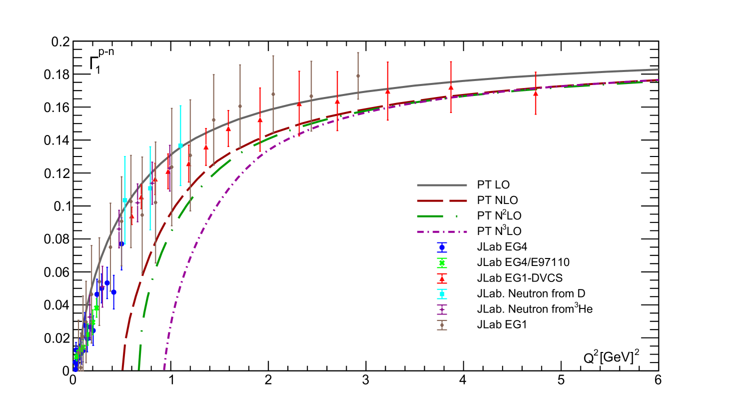
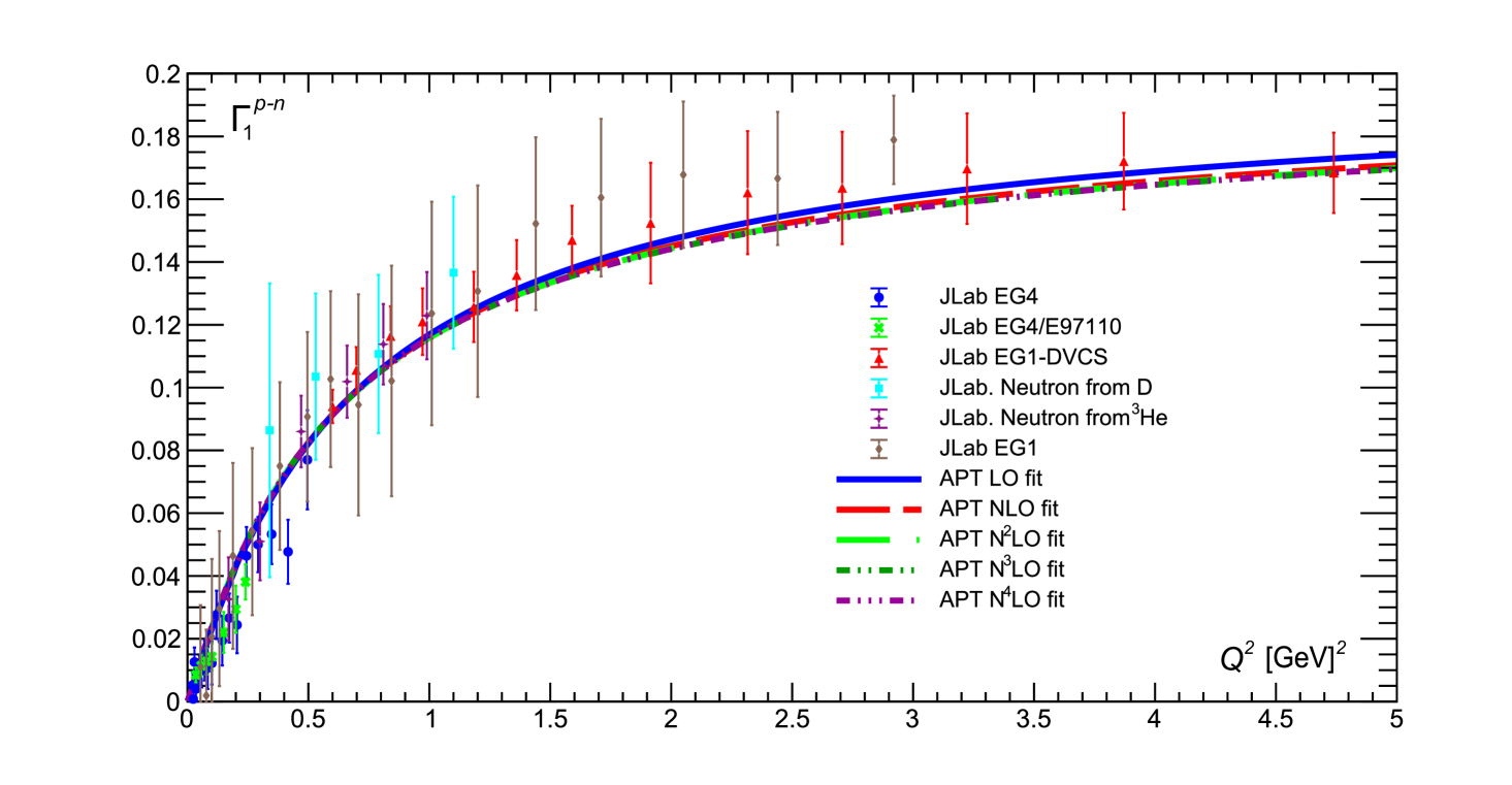
The fitting results of experimental data obtained only with statistical uncertainties are presented in Table 1 and shown in Figs. 1 and 2. For the fits we use -independent and and the two-twist part shown in Eqs. (8), (12) for regular PT and APT, respectively.
As it can be seen in Fig. 1, with the exception of LO, the results obtained using conventional couplant are very poor. Moreover, the discrepancy in this case increases with the order of PT (see also Pasechnik:2008th ; Khandramai:2011zd ; Ayala:2017uzx ; Ayala:2018ulm for similar analyses). The LO results describe experimental points relatively well, since the value of is quite small compared to other , and disagreement with the data begins at lower values of (see Fig. 4 below). Thus, using the “massive” twist-four form (5) does not improve these results, since with conventional couplants become singular, which leads to large and negative results for the twist-two part (7). So, as the PT order increases, ordinary couplants become singular for ever larger values, while BSR tends to negative values for ever larger values.
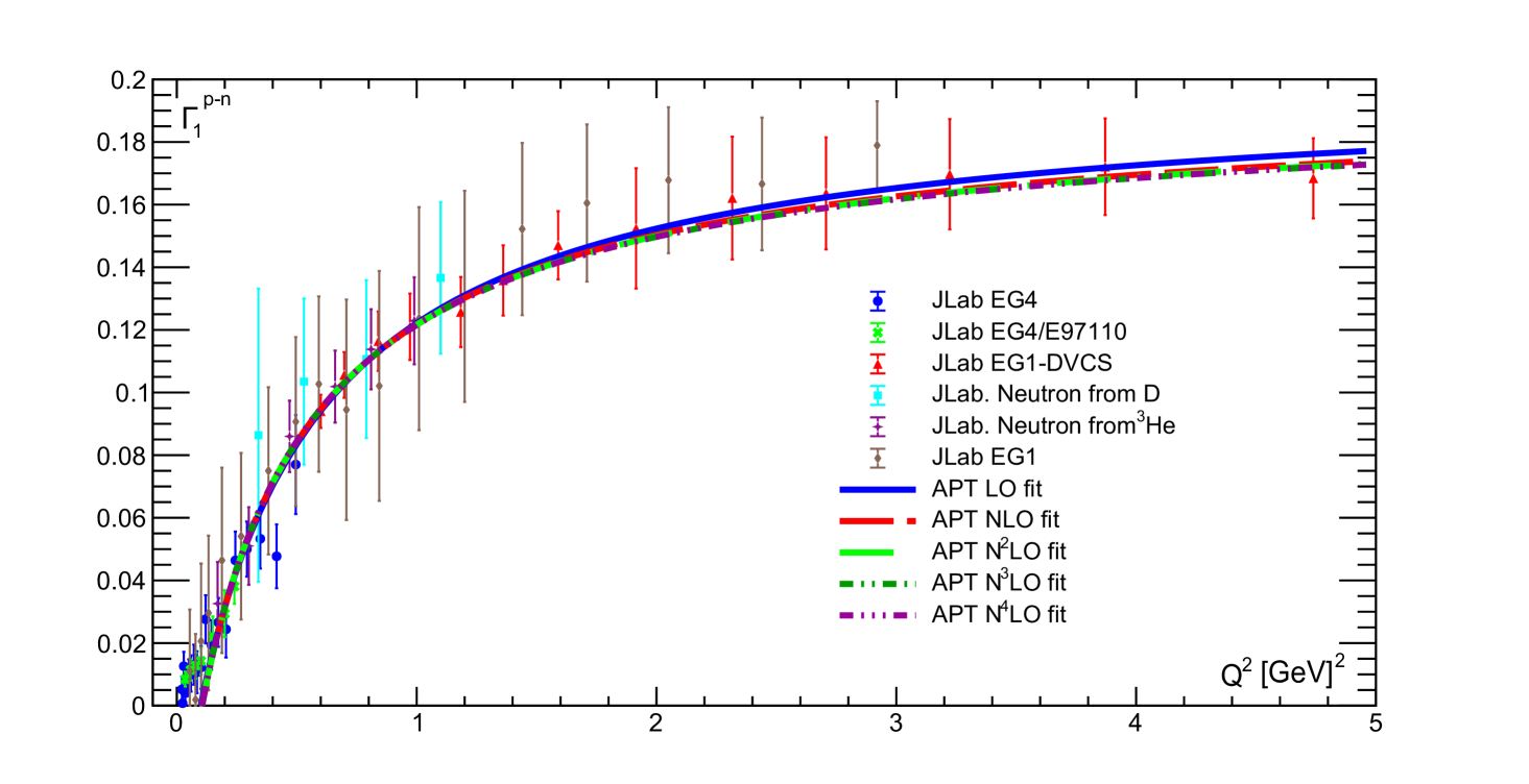
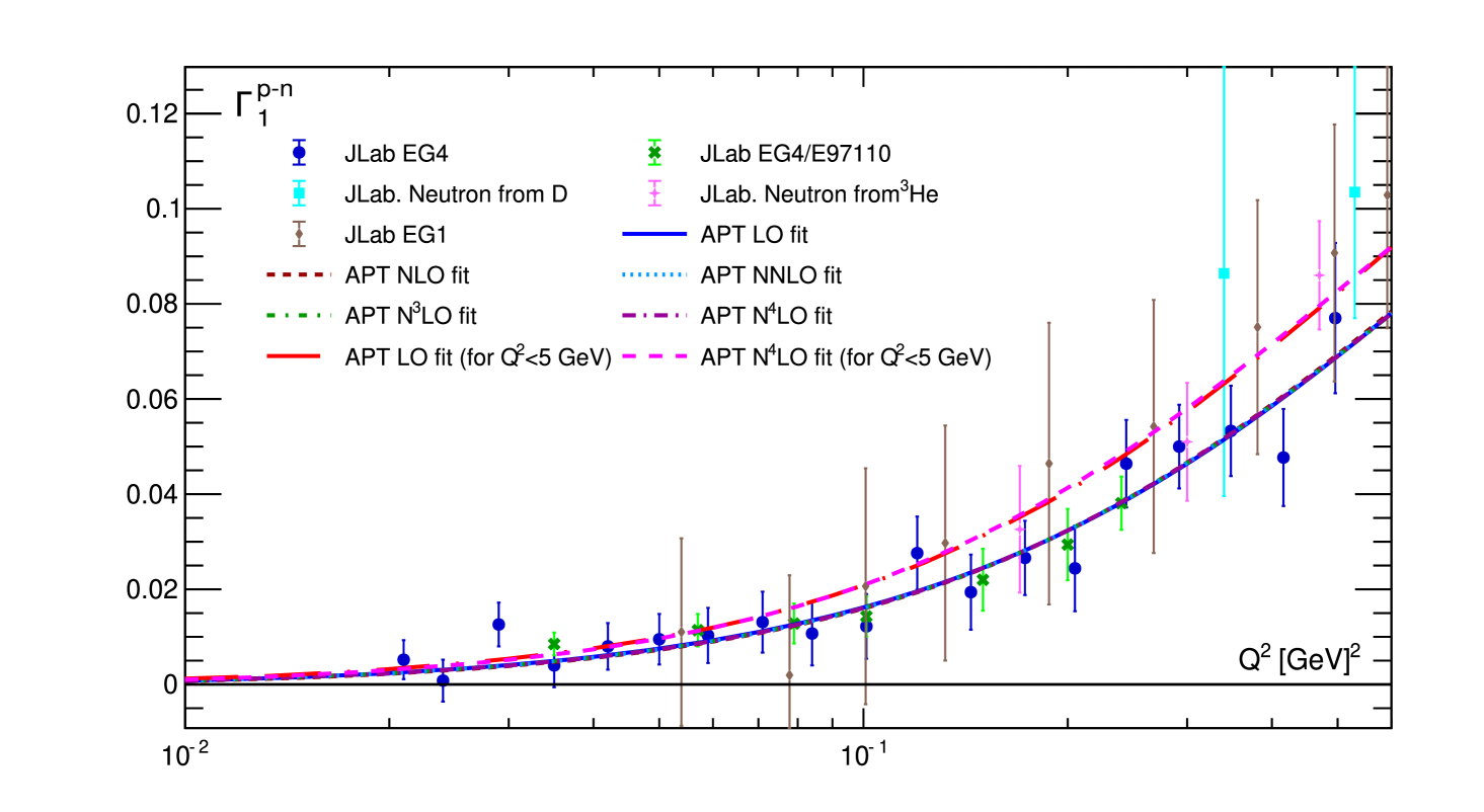
In contrast, our results obtained for different APT orders are practically equivalent: the corresponding curves become indistinguishable when approaches 0 and slightly different everywhere else. As can be seen in Fig. 2, the fit quality is pretty high, which is demonstrated by the values of the corresponding (see Table 1).
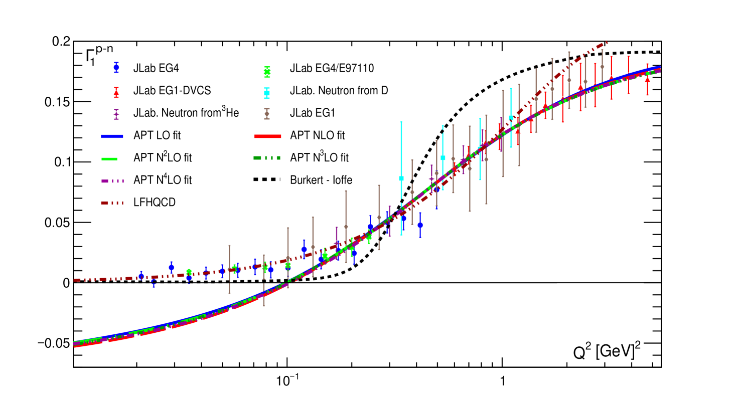
III.1 Low values
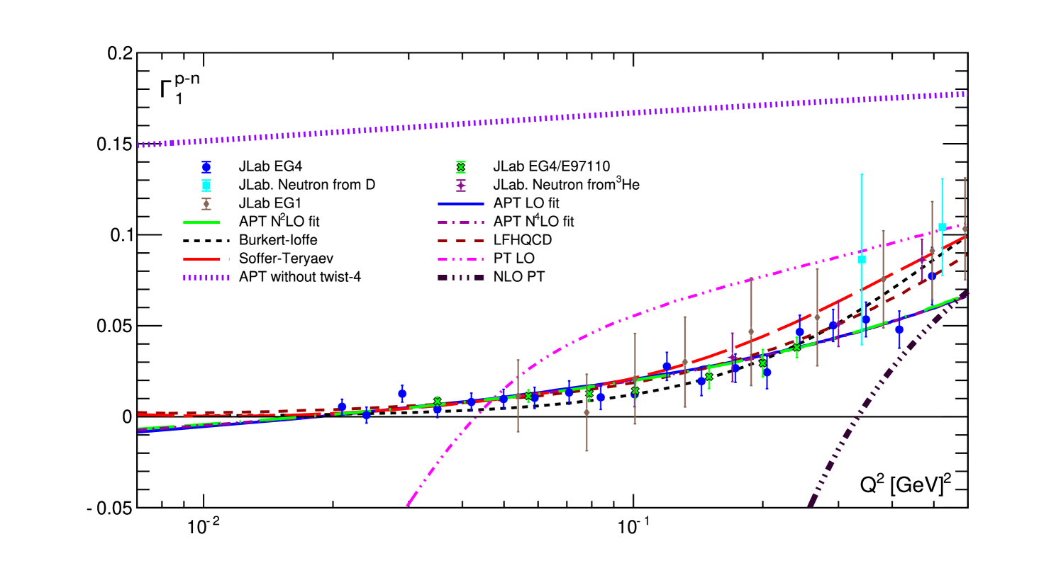
The full picture, however, is more complex than shown in Fig. 2. The APT fitting curves become negative (see Fig. 3) when we move to very low values of : 0.1 GeV2. So, the good quality of the fits shown in Table 1 was obtained due to good agreement with experimenatl data at 0.2 GeV2. The picture improves significantly when we compare our result with experimental data for 0.6 GeV2 (see Fig. 4 and Ref. Gabdrakhmanov:2023rjt ).
Fig. 4 also shows contributions from conventional PT in the first two orders: the LO and NLO predictions have nothing in common with experimental data. As we mentioned above, higher orders lead to even worse agreement, and they are not shown. The purple curve emphasizes the key role of the twist-four contribution (see also Khandramai:2011zd , Kataev:2005ci and the discussions therein). Excluding this contribution, the value of is about 0.16, which is very far from the experimental data.
At GeV2, we also see the good agreement with the phenomenological models: LFHQCD Brodsky:2014yha and the correct IR limit of Burkert–Ioffe model Burkert:1992tg .For larger values of , our results are lower than the results of phenomenological models, and for GeV2 below the experimental data.
Nevertheless, even in this case where very good agreement with experimental data with 0.6 GeV2 is demonstrated, our results for take negative unphysical values when 0.02 GeV2. The reason for this phenomenon can be shown by considering photoproduction within APT, which is the topic of the next subsection.
III.2 Photoproduction
To understand the problem , demonstrated above, we consider the photoproduction case. In the -th order of MA QCD
| (13) |
and, so, we have
| (14) |
The finitness of cross-section in the real photon limit leads to Teryaev:2013qba
| (15) |
For , we have
| (16) |
So, as can be seen from Table 1, the finiteness of the cross section in the real photon limit is violated in our approaches. 444 Note that the results for were obtained taking into account only statistical uncertainties. When adding systematic uncertainties, the results for and are completely consistent with each other, but the predictive power of such an analysis is small. This violation leads to negative values of . Note that this violation is less for experimental data sets with GeV2, where the obtained values for are essentially less then those obtained in the case of experimental data with GeV2. Smaller values of lead to negative values of , when GeV2 (see Fig. 4).
III.3 Gerasimov-Drell-Hearn and Burkhardt-Cottingham sum rules
Now we plan to improve this analysis by involving the result (11) at low values and also taking into account the “massive” twist-six term, similar to the twist-four shown in Eq. (5).
Moreover, we take into account also the Gerasimov-Drell-Hearn (GDH) and Burkhardt-Cottingham (BC) sum rules, which lead to (see Teryaev:2013qba ; Gabdrakhmanov:2017dvg ; Soffer:1992ck ; Pasechnik:2010fg )
| (17) |
where and are proton and neutron magnetic moments, respectively, and = 0.938 GeV is a nucleon mass. Note that the value of is small.
In agreement with the definition (1), we have that
| (18) |
Then, for we obtain at any value, that
| (19) |
but very slowly, that the derivative
| (20) |
Thus, after application the derivative for , every term in becomes to be divergent at . To produce finitness at for the l.h.s. of (17), we can assume the relation between twist-two and twist-four terms, that leads to the appearance of a new contribution
| (21) |
which can be done to be regular at .
The form (21) suggests the following idea about a modification of in (11):
| (22) |
where we added the “massive” twist-six term and introduced different masses in both higher-twist terms and into the modification factor .
The finitness of cross-section in the real photon limit leads now to Teryaev:2013qba
| (23) |
and, thus, we have
| (24) |
| for GeV2 | for GeV2 | |
| (for GeV2) | (for GeV2) | |
| LO | 0.383 0.014 (0.576 0.046) | 0.572 (0.575) |
| NLO | 0.394 0.013 (0.464 0.039) | 0.586 (0.590) |
| N2LO | 0.328 0.014 (0.459 0.038) | 0.617 (0.584) |
| N3LO | 0.330 0.014 (0.464 0.039) | 0.629 (0.582) |
| N4LO | 0.331 0.013 (0.465 0.039) | 0.625 (0.584) |
Using (i.e. ) and putting, for simplicity, , we have
| (26) |
Since the value of is small, so and .
The fitting results of theoretical predictions based on Eq. (22) with and done in (27) (i.e. with the condition ), are presented in Table 2 and on Figs. 5 and 6.
As one can see in Table 2, the obtained results for are different if we take the full data set and the limited one with 0.6 GeV2. However, the difference is significantly less than it was in Table 1. Moreover, the results obtained in the fits using the full data set and shown in Tables 1 and 2 are quite similar, too.
We also see some similarities between the results shown in Figs. 2 and 5. The difference appears only at small values, as can be seen in Figs. 3 and 6.
Fig. 6 also shows that the results of fitting the full set of
experimental data are in better agreement with
the data at GeV2, as it should be, since these data are involved in the analyses of the full set of experimental data.
Of course, the low modification (22) of the result (11) is not unical. There are other possibilities. One of them can be represented as
| (28) |
The finitness of cross-section in the real photon limit leads now to
| (29) |
and, so, we have the relation
| (30) |
IV Conclusions
We have considered the Bjorken sum rule in the framework of MA and perturbative QCD and obtained results similar to those obtained in previous studies Pasechnik:2008th ; Khandramai:2011zd ; Ayala:2017uzx ; Ayala:2018ulm ; Gabdrakhmanov:2023rjt for the first 4 orders of PT. The results based on the conventional PT do not agree with the experimental data. For some values, the PT results become negative, since the high-order corrections are large and enter the twist-two term with a minus sign. APT in the minimal version leads to a good agreement with experimental data when we used the “massive” version (11) for the twist-four contributions.
Examining low behaviour, we found that there is a disagreement between the results obtainded in the fits and application of MA QCD to photoproduction. The results of fits extented to low lead to the negative values for Bjorken sum rule : that contrary to the finitness of cross-section in the real photon limit, which leads to . Note that fits of experimental data at low values (we used 0.6 GeV2) lead to less magnitudes of negative values for .
To solve the problem we considered low modifications of OPE formula for . Considering carefully one of them, Eq. (22), we find good agreemnet with full sets of experimental data for Bjorken sum rule and also with its limit, i.e. with photoproduction. We see also good agreement with phenomenological modeles, especially with LFHQCD Brodsky:2014yha .
As the next step in our research, we plan to add to our analysis the heavy-quark contibution to . It was calculated in a closed form in Ref. Blumlein:2016xcy . It is suppressed by the factor , but contains a contribution of at low values and should be important there.
Acknowledgments Authors are grateful to Alexandre P. Deur for information about new experimental data in Ref. Deur:2021klh and discussions. Authors thank Andrei Kataev and Nikolai Nikolaev for careful discussions. This work was supported in part by the Foundation for the Advancement of Theoretical Physics and Mathematics “BASIS”.
References
- (1) J. D. Bjorken, Phys. Rev. 148, 1467-1478 (1966); Phys. Rev. D 1, 1376-1379 (1970)
- (2) A. Deur, S. J. Brodsky and G. F. De Téramond, [arXiv:1807.05250 [hep-ph]]
- (3) S. E. Kuhn, J. P. Chen and E. Leader, Prog. Part. Nucl. Phys. 63, 1-50 (2009)
- (4) A. Deur et al. Phys. Lett. B 825, 136878 (2022)
- (5) K. Abe et al. [E143 Collaboration], Phys. Rev. D 58, 112003 (1998); K. Abe et al. [E154 Collaboration], Phys. Rev. Lett. 79, 26-30 (1997); P. L. Anthony et al. [E142 Collaboration], Phys. Rev. D 54, 6620-6650 (1996); P. L. Anthony et al. [E155 Collaboration], Phys. Lett. B 463, 339-345 (1999); Phys. Lett. B 493, 19-28 (2000).
- (6) B. Adeva et al. [Spin Muon Collaboration], Phys. Lett. B 302, 533-539 (1993); Phys. Lett. B 412, 414-424 (1997); D. Adams et al. [Spin Muon Collaboration (SMC)], Phys. Lett. B 329, 399-406 (1994) [erratum: Phys. Lett. B 339, 332-333 (1994)]; Phys. Lett. B 357, 248-254 (1995) Phys. Lett. B 396, 338-348 (1997); Phys. Rev. D 56, 5330-5358 (1997)
- (7) E. S. Ageev et al. [COMPASS Collaboration], Phys. Lett. B 612, 154-164 (2005); Phys. Lett. B 647, 330-340 (2007); M. G. Alekseev et al. [COMPASS Collaboration], Phys. Lett. B 690, 466-472 (2010); C. Adolph et al. [COMPASS Collaboration], Phys. Lett. B 753, 18-28 (2016); Phys. Lett. B 769, 34-41 (2017); Phys. Lett. B 781, 464-472 (2018).
- (8) K. Ackerstaff et al. [HERMES Collaboration], Phys. Lett. B 404, 383-389 (1997); A. Airapetian et al. [HERMES Collaboration], Phys. Lett. B 442, 484-492 (1998); Phys. Rev. D 75, 012007 (2007)
- (9) A. Deur et al. Phys. Rev. Lett. 93, 212001 (2004); Phys. Rev. D 78, 032001 (2008) Phys. Rev. D 90, no.1, 012009 (2014)
- (10) K. Slifer et al. [Resonance Spin Structure], Phys. Rev. Lett. 105, 101601 (2010)
- (11) D. V. Shirkov and I. L. Solovtsov, [arXiv:hep-ph/9604363 [hep-ph]]; Phys. Rev. Lett. 79 (1997), 1209-1212; K. A. Milton, I. L. Solovtsov and O. P. Solovtsova, Phys. Lett. B 415 (1997), 104-110; D. V. Shirkov, Theor. Math. Phys. 127 (2001), 409-423; Eur. Phys. J. C 22 (2001), 331-340
- (12) A. P. Bakulev, S. V. Mikhailov and N. G. Stefanis, Phys. Rev. D 72 (2005), 074014 [Erratum-ibid. D 72 (2005), 119908]
- (13) A. P. Bakulev, S. V. Mikhailov and N. G. Stefanis, Phys. Rev. D 75 (2007), 056005 [erratum: Phys. Rev. D 77 (2008), 079901]; JHEP 06 (2010), 085
- (14) G. Cvetic and C. Valenzuela, Braz. J. Phys. 38 (2008), 371-380
- (15) R. S. Pasechnik et al., Phys. Rev. D 78 (2008), 071902; Phys. Rev. D 81 (2010), 016010; A. V. Kotikov and B. G. Shaikhatdenov, Phys. Part. Nucl. 45 (2014), 26-29
- (16) V. L. Khandramai et al., Phys. Lett. B 706 (2012), 340-344
- (17) C. Ayala et al., Int. J. Mod. Phys. A 33 (2018) no.18n19, 1850112; J. Phys. Conf. Ser. 938 (2017) no.1, 012055
- (18) C. Ayala et al., Eur. Phys. J. C 78, no.12, 1002 (2018); J. Phys. Conf. Ser. 1435 (2020) no.1, 012016
- (19) I. R. Gabdrakhmanovet al., JETP Lett. 118, no. 7, 478-482 (2023) [Pisma Zh. Eksp. Teor. Fiz. 118, no.7, 491-492 (2023])
- (20) D. Kotlorz and S. V. Mikhailov, Phys. Rev. D 100, no.5, 056007 (2019)
- (21) C. Ayala, C. Castro-Arriaza and G. Cvetič, Phys. Lett. B 848, 138386 (2024); [arXiv:2312.13134 [hep-ph]].
- (22) G. Cvetic and C. Valenzuela, J. Phys. G 32, L27 (2006); Phys. Rev. D 74 (2006), 114030 [erratum: Phys. Rev. D 84 (2011), 019902]
- (23) P. A. Baikov, K. G. Chetyrkin and J. H. Kuhn, Phys. Rev. Lett. 101, 012002 (2008)
- (24) A. V. Kotikov and I. A. Zemlyakov, Pisma Zh. Eksp. Teor. Fiz. 115 (2022) no.10, 609
- (25) G. Cvetic, R. Kogerler and C. Valenzuela, Phys. Rev. D 82 (2010), 114004
- (26) G. Cvetič and A. V. Kotikov, J. Phys. G 39 (2012), 065005
- (27) A. V. Kotikov and I. A. Zemlyakov, J. Phys. G 50, no.1, 015001 (2023)
- (28) A. V. Kotikov and I. A. Zemlyakov, Phys. Rev. D 107, no.9, 094034 (2023)
- (29) A. V. Kotikov and I. A. Zemlyakov, [arXiv:2207.01330 [hep-ph]]; [arXiv:2302.13769 [hep-ph]].
- (30) E. V. Shuryak and A. I. Vainshtein, Nucl. Phys. B 201, 141 (1982)
- (31) I. I. Balitsky, V. M. Braun and A. V. Kolesnichenko, Phys. Lett. B 242, 245-250 (1990) [erratum: Phys. Lett. B 318, 648 (1993)]
- (32) Particle Data Group collaboration, P.A. Zyla, R.M Barnett, J. Beringer et al., Review of Particle Physics, PTEP 2020 (2020) 083C01.
- (33) O. Teryaev, Nucl. Phys. B Proc. Suppl. 245 (2013), 195-198; V. L. Khandramai, O. V. Teryaev and I. R. Gabdrakhmanov, J. Phys. Conf. Ser. 678 (2016) no.1, 012018
- (34) I. R. Gabdrakhmanov, O. V. Teryaev and V. L. Khandramai, J. Phys. Conf. Ser. 938 (2017) no.1, 012046
- (35) J. P. Chen, [arXiv:nucl-ex/0611024 [nucl-ex]]; J. P. Chen, A. Deur and Z. E. Meziani, Mod. Phys. Lett. A 20 (2005), 2745-2766
- (36) C. Ayala and A. Pineda, Phys. Rev. D 106, no.5, 056023 (2022)
- (37) K. G. Chetyrkin, J. H. Kuhn and C. Sturm, Nucl. Phys. B 744 (2006), 121-135; Y. Schroder and M. Steinhauser, JHEP 01 (2006), 051; B. A. Kniehl et al., Phys. Rev. Lett. 97 (2006), 042001
- (38) H. M. Chen et al., Int. J. Mod. Phys. E 31, no.02, 2250016 (2022)
- (39) A. L. Kataev, JETP Lett. 81, 608-611 (2005); Mod. Phys. Lett. A 20, 2007-2022 (2005)
- (40) V. D. Burkert and B. L. Ioffe, Phys. Lett. B 296, 223-226 (1992); J. Exp. Theor. Phys. 78, 619-622 (1994)
- (41) S. J. Brodsky, G. F. de Teramond, H. G. Dosch and J. Erlich, Phys. Rept. 584, 1-105 (2015)
- (42) J. Soffer and O. Teryaev, Phys. Rev. Lett. 70, 3373-3375 (1993); Phys. Rev. D 70, 116004 (2004)
- (43) R. S. Pasechnik, J. Soffer and O. V. Teryaev, Phys. Rev. D 82, 076007 (2010)
- (44) J. Blümlein, G. Falcioni and A. De Freitas, Nucl. Phys. B 910, 568-617 (2016)