Black-Box Strategies and Equilibrium for Games with Cumulative Prospect Theoretic Players
Abstract
The betweenness property of preference relations states that a probability mixture of two lotteries should lie between them in preference. It is a weakened form of the independence property and hence satisfied in expected utility theory (EUT). Experimental violations of betweenness are well-documented and several preference theories, notably cumulative prospect theory (CPT), do not satisfy betweenness. We prove that CPT preferences satisfy betweenness if and only if they conform with EUT preferences. In game theory, lack of betweenness in the players’ preference relations makes it essential to distinguish between the two interpretations of a mixed action by a player – conscious randomizations by the player and the uncertainty in the beliefs of the opponents. We elaborate on this distinction and study its implication for the definition of Nash equilibrium. This results in four different notions of equilibrium, with pure and mixed action Nash equilibrium being two of them. We dub the other two pure and mixed black-box strategy Nash equilibrium respectively. We resolve the issue of existence of such equilibria and examine how these different notions of equilibrium compare with each other.
1 Introduction
There is a large amount of evidence that human agents as decision-makers do not conform to the independence axiom of expected utility theory (EUT). (See, for example, Allais (1953); Weber and Camerer (1987) and Machina (1992).) This has led to the study of several alternate theories that do away with the independence axiom (Machina, 2014). Amongst these, the cumulative prospect theory (CPT) of Tversky and Kahneman (1992) stands out since it accommodates many of the empirically observed behavioral features from human experiments without losing much analytical tractability (Wakker, 2010). Further, it includes EUT as a special case.
The independence axiom says that if lottery is weakly preferred over lottery by an agent (i.e. the agent wants lottery at least as much as lottery ), and is some other lottery, then, for , the combined lottery is weakly preferred over the combined lottery by that agent. A weakened form of the independence axiom, called betweenness, says that if lottery is weakly preferred over lottery (by an agent), then, for any , the mixed lottery must lie between the lotteries and in preference. Betweenness implies that if an agent is indifferent between and , then she is indifferent between any mixtures of them too. It is known that independence implies betweenness, but betweenness does not imply independence (Chew, 1989). As a result, EUT preferences, which are known to satisfy the independence axiom, also satisfy betweenness. CPT preferences, on the other hand, do not satisfy betweenness in general (see example 2.2). In fact, in theorem 2.3, we show that CPT preferences satisfy betweenness if and only if they are EUT preferences (recall that EUT preferences are a special case of CPT preferences). Several empirical studies show systematic violations of betweenness (Camerer and Ho, 1994; Agranov and Ortoleva, 2017; Dwenger et al., 2012; Sopher and Narramore, 2000), and this makes the use of CPT more attractive than EUT for modeling human preferences. Further evidence comes from Camerer and Ho (1994), where the authors fit data from nine studies using three non-EUT models, one of them being CPT, to find that, compared to the EUT model, the non-EUT models perform better.
Suppose in a non-cooperative game that given her beliefs about the other players, a player is indifferent between two of her actions. Then according to EUT, she should be indifferent between any of the mixtures of these two actions. This facilitates the proof of the existence of a Nash equilibrium in mixed actions for such games. However, with CPT preferences, the player could either prefer some mixture of these two actions over the individual actions or vice versa.
As a result, it is important to make a distinction in CPT regarding whether the players can actively randomize over their actions or not. One way to enable active randomization is by assuming that each player has access to a randomizing device and the player can “commit” to the outcome of this randomization. The commitment assumption is necessary, as is evident from the following scenario (the gambles presented below appear in Prelec (1990)). Alice needs to choose between the following two actions:
-
1.
Action results in a lottery , i.e. she receives with probability and nothing with probability .
-
2.
Action results in a lottery .
(See example 3.7 for an instance of a -player game with Alice and Bob, where Alice has two actions that result in the above two lotteries.) Note that is a less risky gamble with a lower reward and is a more risky gamble with a higher reward. Now consider a compound lottery . Substituting for the lotteries and we get in its reduced form to be
In example 2.1, we provide a CPT model for Alice’s preferences that result in lottery being preferred over lottery , whereas lottery is preferred over lotteries and . Roughly speaking, the underlying intuition is that Alice is risk-averse in general, and she prefers lottery over lottery . However, she overweights the small chance of getting in and finds it lucrative enough to make her prefer lottery over both the lotteries and . Let us say Alice has a biased coin that she can use to implement the randomized strategy. Now, if Alice tossed the coin, and the outcome was to play action 2, then in the absence of commitment, she will switch to action 1, since she prefers lottery over lottery . Commitment can be achieved, for example, by asking a trusted party to implement the randomized strategy for her or use a device that would carry out the randomization and implement the outcome without further consultation with Alice. Regardless of the implementation mechanism, we will call such randomized strategies black-box strategies. The above problem of commitment is closely related to the problem of using non-EUT models in dynamic decisions. For an interesting discussion on this topic, see Wakker (2010, Appendix C) and the references therein.
Traditionally, mixed actions have been considered from two viewpoints, especially in the context of mixed action Nash equilibrium. According to the first viewpoint, these are conscious randomizations by the players – each player only knows her mixed action and not its pure realization. The notion of black-box strategies captures this interpretation of mixed actions. According to the other viewpoint, players do not randomize, and each player chooses some definite action, but the other players need not know which one, and the mixture represents their uncertainty, i.e. their conjecture about her choice. Aumann and Brandenburger (1995) establish mixed action Nash equilibrium as an equilibrium in conjectures provided they satisfy certain epistemic conditions regarding the common knowledge amongst the players.
In the absence of the betweenness condition, these two viewpoints give rise to different notions of Nash equilibria. Throughout we assume that the player set and their corresponding action sets and payoff functions, as well as the rationality of each player, are common knowledge. A player is said to be rational if, given her beliefs and her preferences, she does not play any suboptimal strategy. Suppose each player plays a fixed action, and these fixed actions are common knowledge, then we get back the notion of pure Nash equilibrium (see definition 3.2). If each player plays a fixed action, but the other players have mixed conjectures over her action, and these conjectures are common knowledge, then this gives us mixed action Nash equilibrium (see definition 3.4). This coincides with the notion of Nash equilibrium as defined in Keskin (2016) and studied further in Phade and Anantharam (2019). Now suppose each player can randomize over her actions and hence implement a black-box strategy. If each player plays a fixed black-box strategy and these black-box strategies are common knowledge, then this gives rise to a new notion of equilibrium. We call it black-box strategy Nash equilibrium (see definition 3.8). If each player plays a fixed black-box strategy and the other players have mixed conjectures over her black-box strategy, and these conjectures are common knowledge, then we get the notion of mixed black-box strategy Nash equilibrium (see definition 3.10).
In the setting of an -player normal form game with real valued payoff functions, the pure Nash equilibria do not depend on the specific CPT features of the players, i.e. the reference point, the value function and the two probability weighting functions, one for gains and one for losses. Hence the traditional result on the lack of guarantee for the existence of a pure Nash equilibrium continues to hold when players have CPT preferences. Keskin (2016) proves the existence of a mixed action Nash equilibrium for any finite game when players have CPT preferences. In example 3.9, we show that a finite game may not have any black-box strategy Nash equilibrium. On the other hand, in theorem 3.12, we prove our main result that for any finite game with players having CPT preferences, there exists a mixed black-box strategy Nash equilibrium. If the players have EUT preferences, then the notions of black-box strategy Nash equilibrium and mixed black-box strategy Nash equilibrium are equivalent to the notion of mixed action Nash equilibrium (when interpreted appropriately; see the remark before proposition 3.14; see also figure 6).
The paper is organized as follows. In section 2, we describe the CPT setup and establish that under this setup betweenness is equivalent to independence (theorem 2.3). In section 3, we describe an -player non-cooperative game setup and define various notions of Nash equilibrium in the absence of betweenness, in particular with CPT preferences. We discuss the questions concerning their existence and how these different notions of equilibria compare with each other. In section 4, we conclude with a table that summarizes the results.
To close this section, we introduce some notational conventions that will be used in the document. If is a Polish space (complete separable metric space), let denote the set of all probability measures on , where is the Borel sigma-algebra of . Let denote the support of a distribution , i.e. the smallest closed subset of such that . Let denote the set of all probability distributions that have a finite support. For any element , let denote the probability of assigned by . For , let denote the probability distribution such that . If is finite (and hence a Polish space with respect to the discrete topology), let denote the set of all probability distributions on the set , viz.
with the usual topology. Let denote the standard -simplex, i.e. . If is a subset of a Euclidean space, then let denote the convex hull of , and let denote the closed convex hull of .
2 Cumulative Prospect Theory and Betweenness
We first describe the setup for CPT (for more details see Wakker (2010)). Each person is associated with a reference point , a value function , and two probability weighting functions , for gains and for losses. The function satisfies: (i) it is continuous in , (ii) , (iii) it is strictly increasing in . The value function is generally assumed to be convex in the losses frame () and concave in the gains frame (), and to be steeper in the losses frame than in the gains frame in the sense that for all . However, these assumptions are not needed for the results in this paper to hold. The probability weighting functions satisfy: (i) they are continuous, (ii) they are strictly increasing, (iii) and . We say that are the CPT features of that person.
Suppose a person faces a lottery (or prospect) , where , denotes an outcome and , is the probability with which outcome occurs. We assume that . (Note that we are allowed to have for some values of , and we can have even when .) Let and . We denote as and refer to the vector as an outcome profile and as a probability vector.
Let be a permutation of such that
| (2.1) |
Let be such that for and for . (Here when for all .) The CPT value of the prospect is evaluated using the value function and the probability weighting functions as follows:
| (2.2) |
where and are decision weights defined via:
| for | |||||
| for | |||||
Although the expression on the right in equation (2.2) depends on the permutation , one can check that the formula evaluates to the same value as long as the permutation satisfies (2.1). The CPT value in equation (2.2) can equivalently be written as:
| (2.3) |
A person is said to have CPT preferences if, given a choice between prospect and prospect , she chooses the one with higher CPT value.
We now define some axioms for preferences over lotteries. We are interested in “mixtures” of lotteries, i.e. lotteries with other lotteries as outcomes. Consider a (two-stage) compound lottery , where , are lotteries over real outcomes and is the chance of lottery . We assume that . A two-stage compound lottery can be reduced to a single-stage lottery by multiplying the probability vector corresponding to the lottery by for each , and then adding the probabilities of identical outcomes across all the lotteries . Let denote the reduced lottery corresponding to the compound lottery .
Let denote a preference relation over single-stage lotteries. We assume to be a weak order, i.e. is transitive (if and , then ) and complete (for all , we have or , where possibly both preferences hold). The additional binary relations and are derived from in the usual manner. A preference relation is a CPT preference relation if there exist CPT features such that iff . Note that a CPT preference relation is a weak order. A preference relation satisfies independence if for any lotteries and , and any constant , implies . A preference relation satisfies betweenness if for any lotteries , we have , for all . A preference relation satisfies weak betweenness if for any lotteries , we have , for all .
Suppose a preference relation satisfies independence. Then implies
Thus, if a preference relation satisfies independence, then it satisfies betweenness. Also, if a preference relation satisfies betweenness, then it satifies weak betweenness.
In the following example, we will provide CPT features for Alice so that her preferences agree with those described in section 1. This example also shows that cumulative prospect theory can give rise to preferences that do not satisfy betweenness.
Example 2.1.
Recall that Alice is faced with the following three lotteries:
Let be the reference point of Alice. Thus all the outcomes lie in the gains domain. Let for ; Alice is risk-averse in the gains domain. Let the probability weighting function for gains be given by
a form suggested by Prelec (1998) (see figure 1). We won’t need the probability weighting function for losses. Direct computations show that , and (all decimal numbers in this example are correct to two decimal places). Thus the preference behavior of Alice, as described in section 1 (i.e., she prefers over , but prefers over and ), is consistent with CPT and can be modeled, for example, with the CPT features stated here. ∎
The following example shows that CPT can give rise to preferences that do not satisfy weak betweenness (the lotteries and the CPT features presented below appear in Keskin (2016)).
Example 2.2.
Suppose Charlie has as his reference point and as his value function. Let his probability weighting function for gains be given by
(See figure 1.) We won’t need the probability weighting function for losses since we consider only outcomes in the gains domain in this example. Consider the lotteries and , where (all decimal numbers in this example are correct to three decimal places). Direct computations reveal that .
∎
Given a utility function (assumed to be continuous and strictly increasing), the expected utility of a lottery is defined as . A preference relation is said to be an EUT preference relation if there exists a utility function such that iff . Note that if the CPT probability weighting functions are linear, i.e. for , then the CPT value of a lottery coincides with the expected utility of that lottery with respect to the utility function . It is well known that EUT preference relations satisfy independence and hence betweenness. Several generalizations of EUT have been obtained by weakening the independence axiom and assuming only betweenness, for example, weighted utility theory (Chew and MacCrimmon, 1979; Chew, 1983), skew-symmetric bilinear utility (Fishburn, 1988; Bordley and Hazen, 1991), implicit expected utility (Dekel, 1986; Chew, 1989) and disappointment aversion theory (Gul, 1991; Bordley, 1992). The following theorem shows that in the restricted setting of CPT preferences, betweenness and independence are equivalent.
Theorem 2.3.
If is a CPT preference relation, then the following are equivalent:
-
(i)
is an EUT preference relation,
-
(ii)
satisfies independence,
-
(iii)
satisfies betweenness.
Proof.
Let the CPT preference relation be given by . Since an EUT preference relation satisfies independence, we get that (i) implies (ii). Since betweenness is a weaker condition than independence, we get that (ii) implies (iii). We will now show that if satisfies betweenness, then the probability weighting functions are linear, i.e. for . This will imply that is an EUT preference relation with utility function , and hence complete the proof.
Assume that the CPT preference relation satisfies betweenness. Consider a lottery such that , , and . By (2), we have
where , , and . Let lottery be such that , , and . By (2), we have
If and are such that
| (2.4) |
then and, by betweenness, for any we have , i.e.
Using (2.4) we get
| (2.5) |
Given any , there exist and such that (2.4) holds. Indeed, take any belonging to the range of the function . This exists because and is a strictly increasing function. Since is a strictly increasing function, we have
Take and . These are well defined because is assumed to be continuous and strictly increasing, and belongs to its range. Hence as required. Thus (2) holds for any . In particular, when , we have
where , and . Equivalently, for any such that , we have
In lemma B.1, we prove that the above condition implies , for . Similarly, we can show that , for . This completes the proof. ∎
3 Equilibrium in black-box strategies
We now consider an -player non-cooperative game where the players have CPT preferences. We will discuss several notions of equilibrium for such a game and will contrast them.
Let denote a game, where is the set of players, is the finite action set of player , and is the payoff function for player . Here denotes the set of all action profiles . Let denote the set of action profiles of all players except player .
Definition 3.1.
For any action profile of the opponents, we define the best response action set of player to be
| (3.1) |
Definition 3.2.
An action profile is said to be a pure Nash equilibrium if for each player , we have
The notion of pure Nash equilibrium is the same whether the players have CPT preferences or EUT preferences because only deterministic lotteries, comprised of being offered one outcome with probability , are considered in the framework of this notion. It is well known that for any given game , a pure Nash equilibrium need not exist.
Let denote a belief of player on the action profiles of her opponents. Given the belief of player , if she decides to play action , then she will face the lottery
Definition 3.3.
For any belief , define the best response action set of player as
| (3.2) |
Note that this definition is consistent with the definition of the best response action set that takes an action profile of the opponents as its input (definition 3.1), if we interpret as the belief , since .
Let denote a conjecture over the action of player . Let denote a profile of conjectures, and let denote the profile of conjectures for all players except player . Let be the belief induced by conjectures , given by
which is nothing but the product distribution induced by .
Definition 3.4.
A conjecture profile is said to be a mixed action Nash equilibrium if, for each player , we have
In other words, the conjecture over the action of player should assign positive probabilities to only optimal actions of player , given her belief .
It is well known that a mixed Nash equilibrium exists for every game with EUT players, see Nash (1951). Keskin (2016) generalizes the result of Nash (1951) on the existence of a mixed action Nash equilibrium to the case when players have CPT preferences.
Let denote the set of all black-box strategies for player with a typical element denoted by . Recall that if player implements a black-box strategy , then we interpret this as a trusted party other than the player sampling an action from the distribution and playing action on behalf of player . We assume the usual topology on . Let and with typical elements denoted by and , respectively.
Note that, although a conjecture and a black-box strategy are mathematically equivalent, viz. they are elements of the same set , they have different interpretations. We will call a mixture of actions of player when we want to be agnostic to which interpretation is being imposed. Let and with typical elements denoted by and , respectively. (Note that unless all but one player have singleton action sets.)
For any belief and any black-box strategy of player , let denote the product distribution given by
Given the belief of player , if she decides to implement the black-box strategy , then she will face the lottery .
Definition 3.5.
For any belief , define the best response black-box strategy set of player as
Lemma 3.6.
For any belief , the set is non-empty, and
Proof.
For a lottery , where is the outcome profile, and is the probability vector, the function is continuous with respect to (Keskin, 2016). Thus, is a function continuous with respect to , and hence is a non-empty closed subset of the compact space . Since the convex hull of a compact subset of a Euclidean space is compact (Rudin, 1991, Chapter 3), the set is closed. This completes the proof. ∎
Let us compare the two concepts: the best response action set (definition 3.3) and the best response black-box strategy set (definition 3.5). Even though both of them take the belief of player as input, the best response action set outputs a collection of actions of player , whereas the best response black-box strategy set outputs a collection of black-box strategies of player , which are probability distributions over the set of actions . If we interpret an action as the mixture , and a black-box strategy as a mixture as well, then we can compare the two sets and as subsets of . The following example shows that, in general, the two sets can be disjoint, and hence quite distinct.
Example 3.7.
We consider a -player game. Let Alice be player , with action set , and let Bob be player , with action set . Let the payoff function for Alice be as shown in figure 2. Let be the belief of Alice. Then, as considered in section 1, Alice faces the lottery if she plays action and the lottery if she plays action . We retain the CPT features for Alice, as in example 2.1, viz.: , for , and
We saw that , , and (all decimal numbers in this example are correct to two decimal places). Amongst all the mixtures, the maximum CPT value is achieved at the unique mixture , where ; we have . Thus, and .
∎
For any black-box strategy profile of the opponents, let be the induced belief given by
Definition 3.8.
A black-box strategy profile is said to be a black-box strategy Nash equilibrium if, for each player , we have
If the players have EUT preferences, a conjecture profile is a mixed action Nash equilibrium if and only if the black-box strategy profile , where , for all , is a black-box strategy Nash equilibrium. Thus, under EUT, the notion of a black-box strategy Nash equilibrium is equivalent to the notion of a mixed action Nash equilibrium, although there is still a conceptual difference between these two notions based on the interpretations for the mixtures of actions. Further, we have the existence of a black-box strategy Nash equilibrium for any game when players have EUT preferences from the well-known result about the existence of a mixed action Nash equilibrium. The following example shows that, in general, a black-box strategy Nash equilibrium may not exist when players have CPT preferences.
Example 3.9.
Consider a game (i.e a -player game where each player has two actions ) with the payoff matrices as shown in figure 3. Let the reference points be . Let be the identity function for . Let the probability weighting functions for gains for the two players be given by
where and . We do not need the probability weighting functions for losses since all the outcomes lie in the gains domain for both the players. Notice that player has EUT preferences since .
| 0 | 1 | |
|---|---|---|
| 0 | ||
| 1 |
| 0 | 1 | |
|---|---|---|
| 0 | ||
| 1 |
Suppose player and player play black-box strategies and , respectively, where . With an abuse of notation, we identify these black-box strategies by and , respectively. The corresponding lottery faced by player is given by
where , and . By (2.2), the CPT value of the lottery faced by player is given by
The plot of the function with respect to , for and , is shown in figure 4. We observe that the best response black-box strategy set of player to player ’s black-box strategy satisfies the following: for , for , and for , where and (here the numbers are correct to three decimal points). Further, is singleton for and the unique element in increases monotonically with respect to from to (see figure 5). In particular, . The lottery faced by player is given by
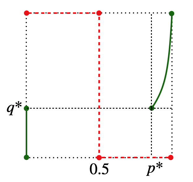
and the CPT value of player for this lottery is given by . The best response black-box strategy set of player to player ’s black-box strategy satisfies the following: for , for , and for . As a result, see figure 5, there does not exist any such that and , and hence no black-box strategy Nash equilibrium exists for this game.
∎
Let denote a conjecture over the black-box strategy of player . This will induce a conjecture over the action of player , given by
Given conjectures over black-box strategies , let .
Definition 3.10.
A profile of conjectures over black-box strategies is said to be a mixed black-box strategy Nash equilibrium if, for each player , we have
Proposition 3.11.
For a profile of conjectures , consider the condition
| (3.3) |
Proof.
Suppose is a mixed black-box strategy Nash equilibrium. Let . Then, for all , we have , and hence . This proves statement (i).
The content of this proposition is that in order to determine whether a profile of conjectures on black box strategies is a mixed black-box strategy Nash equilibrium or not it suffices to study the associated profile of conjectures on actions that is induced by . This justifies the study of the set discussed below.
Theorem 3.12.
For any game , there exists a profile of conjectures that satisfies (3.3).
Proof.
The idea is to use the Kakutani fixed-point theorem, as in the proof of the existence of mixed action Nash equilibrium (Nash, 1950). Assume the usual topology on , for each , and let have the corresponding product topology. The set is a non-empty compact convex subset of the Euclidean space . Let be the set-valued function given by
for all . Since is non-empty and convex for each (lemma 3.6), the function is non-empty and convex for any . We now show that the function has a closed graph. Let and be two sequences in that converge to and , respectively, and let for all . It is enough to show that . For all , let
Since the product distribution is jointly continuous in and , and, as noted earlier, is continuous with respect to the probability vector , for any fixed outcome profile , the function is jointly continuous in and . This implies that the function is jointly continuous in and (see Appendix A). From the definition of , it follows that
Indeed, the maximum on the left-hand side is well-defined since is a compact space and is a continuous function. The maximum on the right-hand side is well-defined and the maximum is achieved by all (lemma 3.6). Hence,
Since , for all , we have
Since is jointly continuous in and , we get
Hence we have . This shows that the function has a closed graph. By the Kakutani fixed-point theorem, there exists such that , i.e. satisfies condition (3.3) (Kakutani, 1941). This completes the proof. ∎
Corollary 3.13.
For any finite game , there exists a mixed black-box strategy Nash equilibrium. In particular, there is one that is a profile of finite support conjectures over the black-box strategies of players.
We now compare the different notions of Nash equilibrium defined above. To that end, we will associate each of the equilibrium notions with their corresponding natural profile of mixtures over actions. For example, corresponding to any pure Nash equilibrium , assign the profile of mixtures over actions . Let denote the set of all profiles of mixtures over actions that correspond to pure Nash equilibria. Let denote the set of all mixed action Nash equilibria . Let denote the set of all black-box strategy Nash equilibria . Corresponding to any mixed black-box strategy Nash equilibrium , assign the profiles of mixtures over actions , and let denote the set of all such profiles. Note that each of the above subsets depends on the underlying game and the CPT features of the players.
Proposition 3.14.
For any fixed game and CPT features of the players, we have
-
(i)
-
(ii)
and
-
(iii)
Proof.
The proof of statement (i) can be found in Keskin (2016).
For statement (ii), let . For a black-box strategy of player , the belief of player gives rise to the lottery . From the definition of CPT value (see equation (2.2)), we observe that is optimal as long as the probability distribution does not assign positive probability to any suboptimal outcome. Hence,
In particular, , and hence .
In the following, we show via examples that each of the labeled regions ((a)–(g)), in figure 6, is non-empty in general.
Example 3.15.
For each of the seven regions in figure 6, we provide a game with the accompanying CPT features for the two players verifying that the corresponding region is non-empty. Let the action sets be . With an abuse of notation, let denote the mixtures over actions for players and , respectively, where and are the probabilities corresponding to action for both the players. Thus, the set of all profiles of mixtures over actions is . Let and denote the corresponding lotteries faced by the two players. (All decimal numbers in these examples are correct to three decimal places.)
-
(a)
Let both the players have EUT preferences with their utility functions given by the identity functions , for . Let the payoff matrix be as shown in figure 7. Clearly, .
- (b)
-
(c)
Let the CPT features for both the players be as in (b). Let the payoff matrix be as shown in figure 7, where and (here as in (b)). As observed in (b), . From the definition of , we see that player is indifferent between her two actions, given her belief over player ’s actions. Thus .
-
(d)
Let , for . Let . Let the payoff matrix be as shown in figure 7, where . Note that the payoffs for player are negations of her payoffs in (b), and her probability weighing function for losses is same as her probability weighing function for gains in (b). Thus her CPT value function is the negation of her CPT value function in (b). In particular, we have for all . Thus, , but . The payoffs and CPT features of player are same as in (b). Thus, .
-
(e)
Let the CPT features for both the players be as in (b). Let the payoff matrix be as shown in figure 7, where , and ; here is the unique maximizer of (see figure 9). We have and with . From the definition of , we see that player is indifferent between her two actions, given her belief over player ’s actions. Thus, .
-
(f)
Let the CPT features be as in example 3.9. Let and be the same as in example 3.9. Let the payoff matrix be as shown in figure 7. Note that the payoffs for both the players are the same as in example 3.9. Recall for , for , and for , and hence and . Further, from the definition of , we have . Hence, .
-
(g)
Finally, if we let the players have EUT preferences and the payoffs as in (a), then .
| 0 | 1 | |
|---|---|---|
| 0 | ||
| 1 |
| 0 | 1 | |
|---|---|---|
| 0 | ||
| 1 |
| 0 | 1 | |
|---|---|---|
| 0 | ||
| 1 |
| 0 | 1 | |
|---|---|---|
| 0 | ||
| 1 |
| 0 | 1 | |
|---|---|---|
| 0 | ||
| 1 |
| 0 | 1 | |
|---|---|---|
| 0 | ||
| 1 |
∎
4 Conclusion
In the study of non-cooperative game theory from a decision-theoretic viewpoint, it is important to distinguish between two types of randomization:
-
1.
conscious randomizations implemented by the players, and
-
2.
randomizations in conjectures resulting from the beliefs held by the other players about the behavior of a given player.
This difference becomes evident when the preferences of the players over lotteries do not satisfy betweenness, a weakened form of independence property. We considered -player normal form games where players have CPT preferences, an important example of preference relation that does not satisfy betweenness. This gives rise to four types of Nash equilibrium notions, depending on the different types of randomizations. We defined these different notions of equilibrium and discussed the question of their existence. The results are summarized in table 1.
| Type of Nash equilibrium | Strategies | Conjectures | Always exists |
|---|---|---|---|
| Pure Nash equilibrium | Pure actions | Exact conjectures | No |
| Mixed action Nash equilibrium | Pure actions | Mixed conjectures | Yes (Keskin, 2016) |
| Black-box strategy Nash equilibrium | Black box strategies | Exact conjectures | No (Example 3.9) |
| Mixed black-box strategy Nash equilibrium | Black box strategies | Mixed conjectures | Yes (Theorem 3.12) |
Appendix A Joint continuity of the concave hull of a jointly continuous function
Let and be simplices of the corresponding dimensions with the usual topologies. Let be a continuous function on (with the product topology). Let denote the space of all probability measures on with the topology of weak convergence. Let be given by
where is the identity function and the expectation is over a random variable taking values in with the distribution .
Proposition A.1.
The function is continuous on .
Proof.
We first prove that the function is upper semi-continuous. Let and . Let be a convergent subsequence of with limit . It is enough to show that the limit . Since for all the set is compact, we know that there exists , such that and . The sequence has a convergent subsequence, say (because is a compact space). Now, . Further, , since the product distributions , for all , on , converge weakly to the product distribution . Thus, and the function is upper-semicontinuous.
We now prove that the function is lower semi-continuous. Let and . The simplex can be triangulated into finitely many other simplices, say , whose vertices are and some of the vertices of . Let be any subsequence such that all for some simplex. It is enough to show that the of the sequence is greater than or equal to . Let the other vertices of be . Let be the barycentric coordinates of with respect to the simplex , i.e.
The function is concave in for any fixed by construction. We have,
Since and are all finite we get,
Let be such that and . Then, , for all , and hence,
This shows that the function is lower semi-continuous.
Since the function is upper and lower semi-continuous, it is continuous. ∎
Appendix B An interesting functional equation
Lemma B.1.
Let be a continuous, strictly increasing function such that and . For any such that , let
| (B.1) |
Then for all .
Proof.
Taking and in (B.1) we get,
and hence,
Note that . Taking and in (B.1) we get,
and hence,
Note that . Taking and in (B.1) we get,
and substituting for we get,
Note that
Taking and in (B.1) we get,
Simplifying we get,
Substituting for and we get,
Since and , we get
Since , we get .
For any fixed , let
Note that is a continuous, strictly increasing function with and . Further, if are such that , then
Thus and hence Using this repeatedly we get for , . Continuity of then implies , for all . ∎
References
- Agranov and Ortoleva [2017] M. Agranov and P. Ortoleva. Stochastic choice and preferences for randomization. Journal of Political Economy, 125(1):40–68, 2017.
- Allais [1953] M. Allais. L’extension des théories de l’équilibre économique général et du rendement social au cas du risque. Econometrica, Journal of the Econometric Society, pages 269–290, 1953.
- Aumann and Brandenburger [1995] R. Aumann and A. Brandenburger. Epistemic conditions for Nash equilibrium. Econometrica: Journal of the Econometric Society, pages 1161–1180, 1995.
- Bordley and Hazen [1991] R. Bordley and G. B. Hazen. SSB and weighted linear utility as expected utility with suspicion. Management Science, 37(4):396–408, 1991.
- Bordley [1992] R. F. Bordley. An intransitive expectations-based Bayesian variant of prospect theory. Journal of Risk and Uncertainty, 5(2):127–144, 1992.
- Camerer and Ho [1994] C. F. Camerer and T.-H. Ho. Violations of the betweenness axiom and nonlinearity in probability. Journal of risk and uncertainty, 8(2):167–196, 1994.
- Chew and MacCrimmon [1979] S. Chew and K. MacCrimmon. Alpha-nu choice theory: an axiomatization of expected utility. University of British Columbia Faculty of Commerce working paper, 669, 1979.
- Chew [1983] S. H. Chew. A generalization of the quasilinear mean with applications to the measurement of income inequality and decision theory resolving the Allais paradox. Econometrica: Journal of the Econometric Society, pages 1065–1092, 1983.
- Chew [1989] S. H. Chew. Axiomatic utility theories with the betweenness property. Annals of operations Research, 19(1):273–298, 1989.
- Dekel [1986] E. Dekel. An axiomatic characterization of preferences under uncertainty: Weakening the independence axiom. Journal of Economic theory, 40(2):304–318, 1986.
- Dwenger et al. [2012] N. Dwenger, D. Kübler, and G. Weizsäcker. Flipping a coin: Theory and evidence. 2012.
- Fishburn [1988] P. C. Fishburn. Nonlinear preference and utility theory. Number 5. Johns Hopkins University Press Baltimore, 1988.
- Gul [1991] F. Gul. A theory of disappointment aversion. Econometrica: Journal of the Econometric Society, pages 667–686, 1991.
- Kakutani [1941] S. Kakutani. A generalization of Brouwer’s fixed point theorem. Duke mathematical journal, 8(3):457–459, 1941.
- Keskin [2016] K. Keskin. Equilibrium notions for agents with cumulative prospect theory preferences. Decision Analysis, 13(3):192–208, 2016.
- Machina [1992] M. J. Machina. Choice under uncertainty: Problems solved and unsolved. In Foundations of Insurance Economics, pages 49–82. Springer, 1992.
- Machina [2014] M. J. Machina. Nonexpected utility theory. Wiley StatsRef: Statistics Reference Online, 2014.
- Nash [1951] J. Nash. Non-cooperative games. Annals of Mathematics, pages 286–295, 1951.
- Nash [1950] J. F. Nash. Equilibrium points in n-person games. Proceedings of the national academy of sciences, 36(1):48–49, 1950.
- Phade and Anantharam [2019] S. R. Phade and V. Anantharam. On the geometry of Nash and correlated equilibria with cumulative prospect theoretic preferences. Decision Analysis, 16(2):142–156, 2019.
- Prelec [1990] D. Prelec. A “pseudo-endowment” effect, and its implications for some recent nonexpected utility models. Journal of Risk and Uncertainty, 3(3):247–259, 1990.
- Prelec [1998] D. Prelec. The probability weighting function. Econometrica, pages 497–527, 1998.
- Rudin [1991] W. Rudin. Functional analysis. 1991. Internat. Ser. Pure Appl. Math, 1991.
- Sopher and Narramore [2000] B. Sopher and J. M. Narramore. Stochastic choice and consistency in decision making under risk: An experimental study. Theory and Decision, 48(4):323–350, 2000.
- Tversky and Kahneman [1992] A. Tversky and D. Kahneman. Advances in prospect theory: Cumulative representation of uncertainty. Journal of Risk and uncertainty, 5(4):297–323, 1992.
- Wakker [2010] P. P. Wakker. Prospect theory: For risk and ambiguity. Cambridge university press, 2010.
- Weber and Camerer [1987] M. Weber and C. Camerer. Recent developments in modelling preferences under risk. Operations-Research-Spektrum, 9(3):129–151, 1987.