Blind Super-resolution via Projected Gradient Descent
Abstract
Blind super-resolution can be cast as low rank matrix recovery problem by exploiting the inherent simplicity of the signal. In this paper, we develop a simple yet efficient non-convex method for this problem based on the low rank structure of the vectorized Hankel matrix associated with the target matrix. Theoretical guarantees have been established under the similar conditions as convex approaches. Numerical experiments are also conducted to demonstrate its performance.
Index Terms— Blind super-resolution, non-convex optimization, projected gradient descent, vectorized Hankel lift.
1 Introduction
Blind super-resolution of point sources is the problem of simultaneously estimating locations and amplitudes of point sources and point spread functions from low-resolution measurements. Such problem arises in various applications, including single-molecule imaging [1], medical imaging [2], multi-user communication system [3] and so on.
Under certain subspace assumption and applying the lifting technique, blind super-resolution can be cast as a matrix recovery problem. Recent works in [4, 5, 6, 7, 8] exploit the intrinsic structures of data matrix and propose different convex relaxation methods for such problem. Theoretical guarantees for these methods have been established. However, due to the limitations of convex relaxation, all of these methods do not scale well to the high dimensional setting.
In contrast to convex relaxation, a non-convex recovery method is proposed in this paper based on the Vectorized Hankel Lift [8] framework. More precisely, harnessing low-rank structure of vectorized Hankel matrix corresponding to the signal in terms of the Burer-Monteiro factorization, we develop a projected gradient descent algorithm, named PGD-VHL, to directly recover the low rank factors. We show that such a simple algorithm possesses a remarkable reconstruction ability. Moreover, our algorithm started from an initial guess converges linearly to the target matrix under the similar sample complexity as convex approaches.
The rest of this paper is organized as follows. We begin with the problem formulation and describe the proposed algorithm in Section 2. Section 3 provides a convergence analysis of PGD-VHL. Numerical experiments to illustrate the performance of PGD-VHL are provided in Section 4. Section 5 concludes this paper.
2 Algorithm
2.1 Problem formulation
The point source signal can be represented as a superposition of spikes
where and are the amplitude and location of -th point source respectively. Let be the unknown point spread functions. The observation is a convolution between and ,
After taking Fourier transform and sampling, we obtain the measurements as
| (2.1) |
Let be a vector corresponding to the -th unknown point spread function. The goal is to estimate as well as from (2.1). Since the number of unknowns is larger than , this problem is an ill-posed problem without any additional assumptions. Following the same route as that in [4, 5, 6, 8], we assume belong to a known subspace spanned by the columns of , i.e.,
Then under the subspace assumption and applying the lifting technique [9], the measurements (2.1) can be rewritten as a linear observations of :
| (2.2) |
where is the -th row of , is the -th standard basis of , and is the vector defined as
The measurement model (2.2) can be rewritten succinctly as
| (2.3) |
where is the linear operator. Therefore, blind super-resolution can be cast as the problem of recovering the data matrix from its linear measurements (2.3).
Let be the vectorized Hankel lifting operator which maps a matrix into an matrix,
where is the -th column of and . It is shown that is a rank- matrix [8] and thus the matrix admits low rank structure when . It is natural to recover by solving the constrained least squares problem
To introduce our algorithm, we assume that is -incoherent which is defined as below.
Assumption 2.1.
Let be the singular value decomposition of , where and . Denote , where is the -th block of for . The matrix is -incoherence if and obey that
for some positive constant .
Remark 2.1.
Letting and , we have
where . Since that target data matrix is -incoherence and the low rank structure of the vectorized Hankel matrix can be promoted by , it is natural to recover the low rank factors of the ground truth matrix by solving an optimization problem in the form of
| (2.4) |
where , is the Moore-Penrose pseudoinverse of obeying that , the second term in objective guarantees that admits vectorized Hankel structure. Last term penalizes the mismatch between and , which is widely used in rectangular low rank matrix recovery [12, 13, 14]. The convex feasible set is defined as follows
| (2.5) |
where is the -th block of , and be two absolute constants such that and .
2.2 Projected gradient descent method
Inspired by [15], we design a projected gradient descent method for the problem (2.1), which is summarized in Algorithm 1.
The initialization involves two steps: (1) computes the best rank approximation of via one step hard thresholding , where is the adjoint of ;(2) projects the low rank factors of best rank- approximated matrix onto the set . Given a matrix , the projection onto , denoted by , has a closed form solution:
for and
for . Let be the current estimator. The algorithm updates along gradient descent direction with step size , followed by projection onto the set . The gradient of is computed with respect to Wirtinger calculus given by where
To obtain the computational cost of , we first introduce some notations. Let be the Hankel operator which maps a vector into an matrix,
where is the -th entry of . The adjoint of , denoted by , is a linear mapping from to . It is known that the computational complexity of both and is flops [16]. Moreover, the authors in [8] show that , where is a matrix constructed by stacking all on top of one another, and is a permutation matrix. Therefore we can compute and by using flops. Thus the implementation of our algorithm is very efficient and the main computational complexity in each step is .
3 Main results
In this section, we provide an analysis of PGD-VHL under a random subspace model.
Assumption 3.1.
The column vectors of are independently and identically drawn from a distribution which satisfies the following conditions
| (3.1) | ||||
| (3.2) |
Remark 3.1.
Assumption 3.1 is a standard assumption in blind super-resolution [4, 5, 6, 17, 8], and holds with by many common random ensembles, for instance, the components of are Rademacher random variables taking the values with equal probability or is uniformly sampled from the rows of a Discrete Fourier Transform (DFT) matrix.
Now we present the main result of the paper.
Theorem 3.1.
Remark 3.2.
Remark 3.3.
Theorem 3.1 implies that PGD-VHL converges to with a linear rate. Therefore, after iterations, we have . Given the iterates returned by PGD-VHL, we can estimate by .
Remark 3.4.
Once the data matrix is recovered, the locations can be computed from by MUSIC algorithm and the weights can be estimated by solving an overdetermined linear system [8].
4 Numerical simulations
In this section, we provide numerical results to illustrate the performance of PGD-VHL. The locations of the point source signal is randomly generated from and the amplitudes are selected to be , where is uniformly sampled from and is uniformly sampled from . The coefficients are i.i.d. sampled from standard Gaussian with normalization. The columns of are uniformly sampled from the DFT matrix. The stepsize of PGD-VHL is chosen via backtracking line search and PGD-VHL will be terminated if is met or a maximum number of iterations is reached. We repeat 20 random trials and record the probability of successful recovery in our tests. A trial is declared to be successful if .
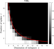
The first experiment studies the recovery ability of PGD-VHL through the framework of phase transition and we compare it with two convex recovery methods: VHL [8] and ANM [5]. Both VHL and ANM are solved by CVX [19]. The tests are conducted with and the varied and . Figure 1(a), 1(c) and 1(e) show that phase transitions of VHL, ANM and PGD-VHL when the locations of point sources are randomly generated, and Figure 1(b), 1(d) and 1(f) illustrate the phase transitions of VHL, ANM and PGD-VHL when the separation condition is imposed. It can be seen that PGD-VHL is less sensitive to the separation condition than ANM and has a higher phase transition curve than VHL.
(a)

(b)

(c)

(d)

(e)

(f)
In the second experiment, we study the phase transition of PGD-VHL when one of and is fixed. Figure 2(a) indicates a approximately linear relationship between and for the successful recovery when the number of point sources is fixed to be . The same linear relationship between and can be observed when the dimension of the subspace is fixed to be , see Figure 2(b). Therefore there exists a gap between our theory and empirical observation and we leave it as future work.

(a)

(b)
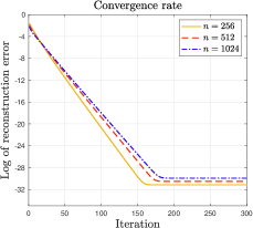
In the third simulation, we investigate the convergence rate of PGD-VHL for different . The results are shown in Figure 3. The -axis denotes and the -axis represents the iteration number. It can be clearly seen that PGD-VHL converges linearly as shown in our main theorem.
5 Conclusion
In this paper, we propose an efficient algorithm named PGD-VHL towards recovering low rank matrix in blind super-resolution. Our theoretical analysis shows that the proposed algorithm converges to the target matrix linearly. This is also demonstrated by our numerical simulations.
References
- [1] Sean Quirin, Sri Rama Prasanna Pavani, and Rafael Piestun, “Optimal 3D single-molecule localization for superresolution microscopy with aberrations and engineered point spread functions,” Proceedings of the National Academy of Sciences, vol. 109, no. 3, pp. 675–679, 2012.
- [2] Xiaobo Qu, Maxim Mayzel, Jian-Feng Cai, Zhong Chen, and Vladislav Orekhov, “Accelerated NMR spectroscopy with low-rank reconstruction,” Angewandte Chemie International Edition, vol. 54, no. 3, pp. 852–854, 2015.
- [3] Xiliang Luo and Georgios B Giannakis, “Low-complexity blind synchronization and demodulation for (ultra-) wideband multi-user ad hoc access,” IEEE Transactions on Wireless communications, vol. 5, no. 7, pp. 1930–1941, 2006.
- [4] Yuejie Chi, “Guaranteed blind sparse spikes deconvolution via lifting and convex optimization,” IEEE Journal of Selected Topics in Signal Processing, vol. 10, no. 4, pp. 782–794, 2016.
- [5] Dehui Yang, Gongguo Tang, and Michael B Wakin, “Super-resolution of complex exponentials from modulations with unknown waveforms,” IEEE Transactions on Information Theory, vol. 62, no. 10, pp. 5809–5830, 2016.
- [6] Shuang Li, Michael B Wakin, and Gongguo Tang, “Atomic norm denoising for complex exponentials with unknown waveform modulations,” IEEE Transactions on Information Theory, vol. 66, no. 6, pp. 3893–3913, 2019.
- [7] Mohamed A Suliman and Wei Dai, “Mathematical theory of atomic norm denoising in blind two-dimensional super-resolution,” IEEE Transactions on Signal Processing, vol. 69, pp. 1681–1696, 2021.
- [8] Jinchi Chen, Weiguo Gao, Sihan Mao, and Ke Wei, “Vectorized hankel lift: A convex approach for blind super-resolution of point sources,” arXiv preprint arXiv:2008.05092, 2020.
- [9] Ali Ahmed, Benjamin Recht, and Justin Romberg, “Blind deconvolution using convex programming,” IEEE Transactions on Information Theory, vol. 60, no. 3, pp. 1711–1732, 2013.
- [10] Emmanuel J Candès and Benjamin Recht, “Exact matrix completion via convex optimization,” Foundations of Computational Mathematics, vol. 9, no. 6, pp. 717, 2009.
- [11] Shuai Zhang, Yingshuai Hao, Meng Wang, and Joe H Chow, “Multichannel Hankel matrix completion through nonconvex optimization,” IEEE Journal of Selected Topics in Signal Processing, vol. 12, no. 4, pp. 617–632, 2018.
- [12] Stephen Tu, Ross Boczar, Max Simchowitz, Mahdi Soltanolkotabi, and Ben Recht, “Low-rank solutions of linear matrix equations via procrustes flow,” in International Conference on Machine Learning. PMLR, 2016, pp. 964–973.
- [13] Qinqing Zheng and John Lafferty, “Convergence analysis for rectangular matrix completion using burer-monteiro factorization and gradient descent,” arXiv preprint arXiv:1605.07051, 2016.
- [14] Yuejie Chi, Yue M Lu, and Yuxin Chen, “Nonconvex optimization meets low-rank matrix factorization: An overview,” IEEE Transactions on Signal Processing, vol. 67, no. 20, pp. 5239–5269, 2019.
- [15] Jian-Feng Cai, Tianming Wang, and Ke Wei, “Spectral compressed sensing via projected gradient descent,” SIAM Journal on Optimization, vol. 28, no. 3, pp. 2625–2653, 2018.
- [16] Jian-Feng Cai, Tianming Wang, and Ke Wei, “Fast and provable algorithms for spectrally sparse signal reconstruction via low-rank Hankel matrix completion,” Applied and Computational Harmonic Analysis, vol. 46, no. 1, pp. 94–121, 2019.
- [17] Mohamed A Suliman and Wei Dai, “Blind two-dimensional super-resolution and its performance guarantee,” arXiv preprint arXiv:1811.02070, 2018.
- [18] Sihan Mao and Jinchi Chen, “Fast blind super-resolution of point sources via projected gradient descent,” Under Preparation, 2021.
- [19] Michael Grant and Stephen Boyd, “CVX: Matlab software for disciplined convex programming, version 2.1,” Mar. 2014.