5pt {textblock}0.80(0.10, 0.01) ©2021 IEEE. Personal use of this material is permitted. Permission from IEEE must be obtained for all other uses, in any current or future media, including reprinting/republishing this material for advertising or promotional purposes, creating new collective works, for resale or redistribution to servers or lists, or reuse of any copyrighted component of this work in other works.
Block Coordinate Descent Algorithms for Auxiliary-Function-Based Independent Vector Extraction
Abstract
In this paper, we address the problem of extracting all super-Gaussian source signals from a linear mixture in which (i) the number of super-Gaussian sources is less than that of sensors , and (ii) there are up to stationary Gaussian noises that do not need to be extracted. To solve this problem, independent vector extraction (IVE) using a majorization minimization and block coordinate descent (BCD) algorithms has been developed, attaining robust source extraction and low computational cost. We here improve the conventional BCDs for IVE by carefully exploiting the stationarity of the Gaussian noise components. We also newly develop a BCD for a semiblind IVE in which the transfer functions for several super-Gaussian sources are given a priori. Both algorithms consist of a closed-form formula and a generalized eigenvalue decomposition. In a numerical experiment of extracting speech signals from noisy mixtures, we show that when in a blind case or at least transfer functions are given in a semiblind case, the convergence of our proposed BCDs is significantly faster than those of the conventional ones.
Index Terms:
Blind source extraction, independent component analysis, independent vector analysis, block coordinate descent method, generalized eigenvalue problemI Introduction
Blind source separation (BSS) is a problem concerned with estimating the original source signals from a mixture signal captured by multiple sensors. When the number of sources is no greater than that of sensors, i.e., in the (over-)determined case, independent component analysis (ICA [1, 2, 3, 4]) has been a popular approach to BSS because it is simple and effective. When each original source is a vector and a multivariate random variable, independent vector analysis (IVA [5, 6]), also termed joint BSS [7, 8, 9], has been widely studied as an extension of ICA.
In this paper, we will only focus on the problem of extracting all the super-Gaussian sources from a linear mixture signal under the following assumptions and improve the computational efficacy of IVA (ICA can also be improved in the same way as IVA, and so we only deal with IVA):
-
1.
The number of super-Gaussian sources is known and fewer than that of sensors , i.e., .
-
2.
There can be up to stationary Gaussian noises, and thus the problem remains (over-)determined.
The second assumption, which concerns the rigorous development of efficient algorithms, can be violated to some extent when applied in practice (see numerical experiments in Section VII). To distinguish it from a general BSS, this problem is called blind source extraction (BSE [2]). The BSE problem is often encountered in such applications as speaker source enhancement, biomedical signal processing, or passive radar/sonar. In speaker source enhancement, for instance, the maximum number of speakers (super-Gaussian sources) can often be predetermined as a certain number (e.g., two or three) while an audio device is equipped with more microphones. In real-word applications, the observed signal is contaminated with background noises, and most noise signals are more stationary than speaker signals.
BSE can be solved by simply applying IVA as if there were super-Gaussian sources and selecting the top super-Gaussian signals from the separated signals in some way. However, this approach is computationally intensive if gets too large. To reduce the computing cost, for preprocessing of IVA, the number of channels (or sensors) can be reduced to by using principle component analysis or by selecting sensors with high SNRs. These channel reductions, however, often degrade the separation performance due to the presence of the background noises.
BSE methods for efficiently extracting just one or several non-Gaussian signals (not restricted to super-Gaussian signals) have already been studied mainly in the context of ICA [10, 11, 12, 13, 14, 15, 16, 17, 18, 19, 20]. The natural gradient algorithm and the FastICA method with deflation techniques [16, 17, 18] can sequentially extract non-Gaussian sources one by one. In FastICA, the deflation is based on the orthogonal constraint where the sample correlation between every pair of separated signals equals zero. This constraint was also used to develop FastICA with symmetric orthonormalization [17, 18, 19, 20] that can simultaneously extract non-Gaussian signals.
I-A Independent vector extraction (IVE)
Recently, maximum likelihood approaches have been proposed for BSE in which the background noise components are modeled as stationary Gaussians. These methods include independent vector extraction (IVE [21, 22, 23]) and overdetermined IVA (OverIVA [24, 25, 26, 27]), which will be collectively referred to as IVE in this paper. When non-Gaussian sources are all super-Gaussian (as defined in Assumption 2), IVE can use a majorization-minimization (MM [28]) optimization algorithm developed for an auxiliary-function-based ICA (AuxICA [29]) and an auxiliary-function-based IVA (AuxIVA [30, 31, 32]). In this paper, we only deal with an IVE based on the MM algorithm [24, 25, 26, 27, 23] and always assume that the super-Gaussian distributions are defined by Assumption 2 in Section III-A.
In the MM-based IVE, each separation matrix is optimized by iteratively minimizing a surrogate function of the following form:
Here, are filters that extract the target-source signals and is a filter that extracts the noise components. are the Hermitian positive definite matrices that are updated in each iteration of the MM algorithm. Interestingly, when or when viewing the second term of as , the problem of minimizing has been discussed in ICA/IVA literature [33, 34, 35, 36, 37]. Among the algorithms developed so far, block coordinate descent (BCD [38]) methods with simple analytical solutions have attracted much attention in the field of audio source separation because they have been experimentally shown to give stable and fast convergence behaviors. A family of these BCD algorithms [29, 30, 31, 32], summarized in Table I, is currently called an iterative projection (IP) method. The IP method has been widely applied not only to ICA and IVA but also to audio source separation methods using more advanced source models (see [39, 40, 41, 42, 43] for the details of such methods).
I-B Conventional BCD (or IP) algorithms for IVE
When we consider directly applying the IP methods developed for AuxIVA to the BSE problem of minimizing with respect to , AuxIVA-IP1 [30] in Table I, for instance, will cyclically update one by one. However, in the BSE problem, the signals of interests are non-Gaussian sources, and most of the optimization of should be skipped.
Therefore, in a previous work [24], an algorithm (IVE-OC in Table I) was proposed that cyclically updates one by one with a computationally cheap formula for . In this work [24], the updating equation for was derived solely from the (weak) orthogonal constraint (OC [22, 21, 23]) where the sample correlation between the separated non-Gaussian sources and the background noises equals zero. (Note that the non-Gaussian sources are not constrained to be orthogonal in the OC.) Although the algorithm has successfully reduced the computational cost of IVA by nearly a factor of , the validity of imposing the heuristic OC remains unclear.
After that, IVE-OC has been extended by removing the OC from the model. One such extension is a direct method that can obtain a global minimizer of when [25, 27]. The other extension is a BCD algorithm for that cyclically updates the pairs one by one [26], but the computational cost is not so cheap due to the full update of in each iteration. These algorithms are called IVE-IP2 in this paper (see Table I).
I-C Contributions
In this work, we propose BCD algorithms for IVE, which are summarized in Table I with comparisons to the previous BCDs (IPs). The followings are the contributions of this paper.
(i) We speed up the previous IVE-IP2 for by showing that ’s update can be omitted in each iteration of BCD without changing the behaviors of the algorithm (Section IV-F). This is attained by carefully exploiting the stationary Gaussian assumption for the noise components. In an experiment of speaker source enhancement, we confirmed that the computational cost of the conventional IVE-IP2 is consistently reduced.
(ii) We provide a comprehensive explanation of IVE-IP2 for (Sections IV-D and IV-H). Interestingly, it turns out to be a method that iteratively updates the maximum signal-to-noise-ratio (MaxSNR [44, 45]) beamformer and the power spectrum for the unique () target-source signal. The experimental result shows that this algorithm has much faster convergence than conventional algorithms. Note that IVE-IP2 for was developed independently and simultaneously in our conference paper [27] and by Scheibler–Ono [25].
(iii) We reveal that IVE-OC [24], which was developed with the help of the heuristic orthogonal constraint (OC), can also be obtained as a BCD algorithm for our proposed IVE without the OC (Section IV-G). (This interpretation of IVE-OC as a BCD algorithm was described in our conference paper [27], but it is not mathematically rigorous. We here provide a rigorous proof of this interpretation.)
(iv) We further extend the proposed IVE-IP2 for the semiblind case where the transfer functions for () sources of interests can be given a priori (Section V). We call the proposed semiblind method Semi-IVE. In Semi-IVE, separation filters, e.g., , which correspond to the known transfer functions are optimized by iteratively solving the linear constrained minimum variance (LCMV [44]) beamforming algorithm, and the remaining (and ) are optimized by the full-blind IVE-IP2 algorithm. We experimentally show that when transfer functions are given Semi-IVE yields surprisingly fast convergence.
Organization: The rest of this paper is organized as follows. The BSE and semi-BSE problems are defined in Section II. The probabilistic model for the proposed IVE is compared with related methods in Section III. The optimization algorithms are developed separately for the BSE and semi-BSE problems in Sections IV and V. The computational time complexity for these methods is discussed in Section VI. In Sections VII and VIII, experimental results and concluding remarks are described.
I-D Notations
Let or denote the set of all Hermitian positive semidefinite (PSD) or positive definite (PD) matrices of size . Let denote the set of all (complex) nonsingular matrices of size . Also, let be the zero vector, let be the zero matrix, let be the identity matrix, and let be a vector whose -th element equals one and the others are zero. For a vector or matrix , and represent the transpose and the conjugate transpose of . The element-wise conjugate is denoted as . For a matrix , is defined as the subspace . For a vector , denotes the Euclidean norm.
| Method | Algorithm | Reference | Assumption | Optimization process of BCD | |
| Conventional | (Aux)IVA | IP1 | [30] | - | |
| IP2 | [31] | (direct optimization) | |||
| IP2 | [32] | (if is even) | |||
| Conventional | IVE | IVE-OC1) | [24], §III-C | Orthogonal constraint (OC) | |
| IP23) | [26], §IV-E | ||||
| Proposed | IVE | IP11) | §IV-G | - | |
| IP22) | §IV-D | (direct optimization) | |||
| IP23) | §IV-F | ||||
| Proposed | Semi-IVE | IP24) | §V | Given | (direct optimization) |
| §V | Given | ||||
| 1) The two algorithms are identical as shown in Section IV-G. | |||||
| 2) It was developed independently and simultaneously by Scheibler–Ono [25] and the authors [27] in Proceedings of ICASSP2020. | |||||
| 3) The proposed IVE-IP2 for is an acceleration of the conventional IVE-IP2 developed in [26]. | |||||
| 4) , which correspond to , are directly globally optimized as the LCMV beamformers (see Section V-B). | |||||
| 2,3,4) In the proposed IVE-IP2 and Semi-IVE, the optimizations for are skipped (see Sections IV-D, IV-F, and V-C). | |||||
II Blind and semiblind source extraction
II-A Blind source extraction (BSE) problem
Throughout this paper, we discuss IVA and IVE using the terminology from audio source separation in the short-term Fourier transform (STFT) domain.
Suppose that super-Gaussian target-source signals and a stationary Gaussian noise signal of dimension are transmitted and observed by sensors. In this paper, we only consider the case where . The observed signal in the STFT domain is modeled at each frequency bin and time-frame as
| (1) | ||||
| (2) | ||||
| (3) | ||||
| (4) |
where and are the STFT coefficients of target source and the noise signal, respectively. is the (time-independent) acoustic transfer function (or steering vector) of source to the sensors, and is that of the noise. It is assumed that the source signals are statistically mutually independent.
In the blind source extraction (BSE) problem, we are given an observed mixture and the number of target sources . From these inputs, we seek to estimate the spatial images for the target sources, which are defined as , .
II-B Semiblind source extraction (Semi-BSE) problem
In the semiblind source extraction (Semi-BSE) problem, in addition to the BSE inputs, we are given transfer functions for super-Gaussian sources, where . From these inputs, we estimate all the target-source spatial images . If , then Semi-BSE is known as a beamforming problem.
Motivation to address Semi-BSE: In some applications of audio source extraction, such as meeting diarization [46], the locations of some (but not necessarily all) point sources are available or can be estimated accurately, and their acoustic transfer functions can be obtained from, e.g., the sound propagation model [47]. For instance, in a conference situation, the attendees may be sitting in chairs with fixed, known locations. On the other hand, the locations of moderators, panel speakers, or audience may change from time to time and cannot be determined in advance. In such a case, by using these partial prior knowledge of transfer functions, Semi-BSE methods can improve the computational efficiency and separation performance of BSE methods. In addition, since there are many effective methods for estimating the transfer function of (at least) a dominant source [48, 49, 50], there is a wide range of applications where Semi-BSE can be used to improve the performance of BSE.
III Probabilistic models
We start by presenting the probabilistic models for the proposed auxiliary-function-based independent vector extraction (IVE), which is almost the same as those of such related methods as IVA [5], AuxIVA [30, 31, 32], and the conventional IVE [22, 21, 23, 24, 25, 26].
III-A Probabilistic model of proposed IVE
In the mixing model (1), the mixing matrix
| (5) |
is square and generally invertible, and hence the problem can be converted into one that estimates a separation matrix satisfying , or equivalently, satisfying
| (6) | ||||
| (7) |
where we define
| (8) | ||||
| (9) | ||||
| (10) |
Denote by the vector of all the frequency components for source and time-frame . The proposed IVE exploits the following three assumptions. Note that Assumption 2 was introduced for developing AuxICA [29] and AuxIVA [30, 31, 32].
Assumption 1 (Independence of sources).
The random variables are mutually independent:
Assumption 2 (Super-Gaussian distributions for the target sources [29, 30]).
The target-source signal follows a circularly symmetric super-Gaussian distribution:
| (11) |
where is differentiable and satisfies that is nonincreasing on . Here, is the first derivative of . Candidates of (or the probability density functions) include the function and the circularly symmetric generalized Gaussian distribution (GGD) with the scale parameter and the shape parameter , which is also known as the exponential power distribution [51]:
| (12) |
GGD is a parametric family of symmetric distributions, and when it is nothing but the complex Laplace distribution. It has been experimentally shown in many studies that ICA type methods including IVA and IVE can work effectively for audio source separation tasks when audio signals such as speech signals are modeled by the super-Gaussian distributions (see, e.g., [5, 6, 21, 22, 23, 24, 25, 26, 27, 30, 31, 32]).
Assumption 3 (Stationary Gaussian distribution for the background noise).
The noise signal follows a circularly symmetric complex Gaussian distribution with the zero mean and identity covariance matrix:
| (13) | ||||
| (14) |
Assumption 3 plays a central role for deriving several efficient algorithms for IVE. Despite this assumption, as we experimentally confirm in Section VII, the proposed IVE can extract speech signals even in a diffuse noise environment where the noise signal is considered super-Gaussian or nonstationary and has an arbitrary large spatial rank.
With the model defined by (6)–(13), the negative loglikelihood, , can be computed as
| (15) | ||||||
where are the variables to be optimized.
Remark 1.
III-B Relation to IVA and AuxIVA
If we assume that the noise components also independently follow super-Gaussian distributions, then the IVE model coincides with that of IVA [5] or AuxIVA [30, 31, 32]. The following are the two advantages of assuming the stationary Gaussian model (13).
(i) As we confirm experimentally in Section VII, when we optimize the IVE model, separation filters extract the top highly super-Gaussian (or nonstationary) signals such as speech signals from the observed mixture while extracts only the background noises that are more stationary and approximately follow Gaussian distributions. On the other hand, in IVA, which assumes super-Gaussian noise models, () target-source signals need to be chosen from the separated signals after optimizing the model.
III-C Relation to IVE with orthogonal constraint
The proposed IVE is inspired by OverIVA with an orthogonal constraint (OC) [24]. This conventional method will be called IVE-OC in this paper.
IVE-OC [24] was proposed as an acceleration of IVA [30] for the case where , while maintaining its separation performance. The IVE-OC model is defined as the proposed IVE by replacing the noise model from (13) to (16) and introducing two additional constraints:
| (18) | ||||
| (19) |
The first constraint (18) may be applicable because there is no need to extract the noise components (see [24, 26] for details). The second constraint (19), called an orthogonal constraint (OC [21]), was introduced to help the model distinguish between the target-source and noise signals.
OC, which forces the sample correlation between the separated target-source and noise signals to be zero, can equivalently be expressed as
| (20) | ||||
| (21) | ||||
| (22) |
which together with (18) imply
| (23) |
where we define
| (24) | ||||
| (25) |
From (18) and (23), it turns out that is uniquely determined by in the IVE-OC model. Hence, in a paper on IVE-OC [24], an algorithm was proposed in which is updated based on (18) and (23) immediately after updating any other variables to always impose OC on the model. Although the algorithm was experimentally shown to work well, its validity from a theoretical point of view is unclear because the update rule for is derived solely from the constraints (18)–(19) and does not reflect an objective of the optimization problem for parameter estimation, such as minimizing the negative loglikelihood.
In this paper, we develop BCD algorithms for the maximum likelihood estimation of the proposed IVE that does not rely on OC, and identify one such algorithm (IVE-IP1 developed in Section IV-G) that exactly coincides with the conventional algorithm for IVE-OC. This means that OC is not essential for developing fast algorithms in IVE-OC. Due to removing OC from the model, we can provide other more computationally efficient algorithms for IVE, which is the main contribution of this paper.
IV Algorithms for the BSE problem
We develop iterative algorithms for the maximum likelihood estimation of IVE. The proposed and some conventional algorithms [24, 25, 26, 27] are based on the following two methods.
- •
-
•
The other is block coordinate descent (BCD) algorithms. In each iteration of BCDs, several columns are updated to globally minimize the above surrogate function with respect to that variable. In this paper, we propose several BCDs that improve the conventional BCDs.
Our proposed algorithms are summarized in Algorithm 1. The optimization processes of all the BCDs are summarized in Table I and detailed in the following subsections. The computational time complexities of the algorithms are discussed in Section VI.
IV-A Majorization-minimization (MM) approach
We briefly describe how to apply the conventional MM technique developed for AuxICA [29] to the proposed IVE.
In IVE as well as AuxICA/AuxIVA, a surrogate function of is designed with an auxiliary variable that satisfies
| (26) |
Then, variables and are alternately updated by iteratively solving
| (27) | ||||
| (28) |
for until convergence. In the same way as in AuxIVA [30], by applying Proposition 5 in Appendix A to the first term of , problem (28) in IVE comes down to solving the following subproblems:
| (29) |
where and
| (30) | ||||
| (31) | ||||
| (32) | ||||
| (33) | ||||
| (34) |
Here, the computation of (33)–(34) corresponds to the optimization of (27). Recall that in (33) is the first derivative of (see Assumption 2). To efficiently solve (29), we propose BCD algorithms in the following subsections. From the derivation, it is guaranteed that the objective function is monotonically nonincreasing at each iteration in the MM algorithm.111 Due to space limitations, showing the convergence rate and other convergence properties of the proposed algorithms will be left as a future work.
IV-B Block coordinate descent (BCD) algorithms and the stationary condition for problem (29)
No algorithms have been found that obtain a global optimal solution for problem (29) for general . Thus, iterative algorithms have been proposed to find a local optimal solution. Among them, a family of BCD algorithms has been attracting much attention (e.g., [29, 30, 31, 32, 24, 26, 25, 27, 39, 40, 41, 42]) because they have been experimentally shown to work faster and more robustly than other algorithms such as the natural gradient method [52]. The family of these BCD algorithms (specialized to solve (29)) is currently called an iterative projection (IP) method.
As we will see in the following subsections, all the IP algorithms summarized in Table I can be developed by exploiting the stationary condition, which is also called the first-order necessary optimality condition [53]. To simplify the notation, when we discuss (29), we abbreviate frequency bin index without mentioning it. For instance, and are simply denoted as and (without confusion).
To rigorously derive the algorithms, we always assume the following two technical but mild conditions (C1) and (C2) for problem (29):222 If (C1) is violated, problem (29) has no optimal solutions and algorithms should diverge to infinity (see [54, Proposition 1] for the proof). Conversely, if (C1) is satisfied, it is guaranteed that problem (29) has an optimal solution by Proposition 6 in Appendix A. In practice, the number of frames exceeds that of sensors , and (C1) holds in general. Condition (C2) is satisfied automatically if we initialize as nonsingular. Intuitively, singular implies , which will never occur during optimization.
- (C1)
-
are positive definite.
- (C2)
-
Estimates of are always nonsingular during optimization.
IV-C Conventional methods: IVA-IP1, IVA-IP2, and IVE-OC
IV-C1 IVA-IP1
Let . As shown in Table I, IVA-IP1 [30] cyclically updates each separation filter by solving the following subproblem for each one by one:
| (37) |
This can be solved under (C1) and (C2) by
| (38) | ||||
| (39) |
Here, we define for , and the th column of in (38), i.e., , is set to the current value before update. When applied to the BSE problem, IVA-IP1’s main drawback is that the computation time increases significantly as gets larger since it updates even though there is no need to extract the background noises.
IV-C2 IVE-OC
To accelerate IVA-IP1 when it is applied to the BSE problem, IVE-OC [24] updates using (18) and (23) (see Section III-C and Algorithm 2). Although this update rule seems heuristic, we reveal in Section IV-G that IVE-OC can be comprehended in terms of BCD for the proposed IVE that does not rely on OC.
IV-C3 IVA-IP2
IV-D Proposed IVE-IP2 for the case of
We focus on the case where and derive the proposed algorithm IVE-IP2333 The algorithm IVE-IP2 for was developed independently and simultaneously by Scheibler–Ono (called the fast IVE or FIVE [25]) and the authors [27] in the Proceedings of ICASSP2020. In this paper, we give a complete proof for the derivation of IVE-IP2 and add some remarks (see also Section IV-H for the projection back operation). that is expected to be more efficient than IVE-IP1. The algorithm is summarized in Algorithm 3.
When or , problem (29) can be solved directly through a generalized eigenvalue problem [35, 31, 32]. We here extend this direct method to the case where and in the following proposition.
Proposition 2.
Proof.
We prove the “only if” part. The stationary conditions (35)–(36) imply that vectors and are orthogonal to the subspace of dimension . Hence, it holds that for some , where is given by (44). This is restricted by , and we obtain (41). In a similar manner, (36) implies that vector is orthogonal to of dimension . Hence, it holds that for some , where is given by (43). This is restricted by , and we have (42).
We next show the latter statement. By Proposition 6 in Section IV-G, global optimal solutions exist, and they must satisfy the stationary conditions, which are equivalent to (41)–(44). Since (41)–(44) satisfy (35)–(36), the sum of the first and second terms of becomes , which is constant. On the other hand, for the term, it holds that
where we define and use in the second equality. Hence, the largest leads to the smallest , which concludes the proof. ∎
By Proposition 2, under condition (C1), a global optimal solution for problem (29) can be obtained by updating using (41)–(44) with and and choosing the generalized eigenvalue in (44) as the largest one. Moreover, this algorithm can be accelerated by omitting the computation of (42)–(43) and updating only according to (41) and (44). It is applicable for extracting the unique target-source signal because the formulas for computing , , and are independent of . The obtained algorithm IVE-IP2 is shown in Algorithm 3.
IV-E Drawback of conventional IVE-IP2 for the case of
Suppose . The conventional IVE-IP2 developed in [26, Algorithm 2] is a BCD algorithm that cyclically updates the pairs by solving the following subproblem for each one by one:
| (45) |
It was shown in [26, Theorem 3] that a global optimal solution of problem (45) can be obtained through a generalized eigenvalue problem. In this paper, we simplify the result of [26, Theorem 3] in the next proposition, based on which we will speed up the conventional IVE-IP2 in Section IV-F.
Proposition 3.
Let , and . A global optimal solution of problem (45) is obtained as
| (46) | ||||
| (47) | ||||
| (48) | ||||
| (49) | ||||
| (50) | ||||
| (51) | ||||
| (52) |
where is defined by (25), and and in (50) are set arbitrarily as long as is nonsingular (for instance they can be set to the current values under condition (C2)). Also, (52) is the generalized eigenvalue problem for , and is the eigenvector corresponding to the largest generalized eigenvalue .
Proof.
The proof is given in Appendix B. ∎
In the conventional IVE-IP2, under condition (C2), problem (45) is solved by (46)–(50) where is computed through the following generalized eigenvalue problem instead of using (51)–(52):
| (53) |
Since the computational cost of solving (53) is greater than computing (51)–(52), we can speed up the conventional IVE-IP2, as shown in the next subsection.
IV-F Proposed IVE-IP2 for
The proposed IVE-IP2 for , which is summarized in Algorithm 4, is an acceleration of the conventional IVE-IP2 described in the previous subsection. We here provide another efficient formula to solve (45) without changing the behavior of the conventional IVE-IP2.
Thanks to newly providing Proposition 3, we can update the pair according to (46)–(52) in which only the first generalized eigenvector has to be computed. Moreover, for the purpose of optimizing , we do not have to update using Eqs. (47) and (51) when solving problem (45) for each . To see this, observe that
- 1.
-
2.
never contributes to the construction of the surrogate function during iterative optimization.
This observation implies that problem (45) remains the same during iterative optimization regardless whether we update or not. Hence, in IVE-IP2, it is sufficient to update only in (45) using Eqs. (46), (48)–(50), (52).
This advantage stems from the stationary Gaussian assumption for the noise components. To the contrary, suppose that the noise components are nonstationary or non-Gaussian. Then, the surrogate function as well as should depend on in the same way that depends on , meaning that must be optimized in subproblem (45). In this way, the stationary Gaussian assumption is important to derive a computationally efficient algorithm for IVE.
IV-G IVE-IP1: Reinterpretation of the conventional IVE-OC
In this subsection, we model the noise components by (16) with a general time-independent covariance matrix , i.e.,
| (54) |
and develop a BCD algorithm called IVE-IP1 that cyclically updates by solving the following subproblems one by one:
| (55) | ||||
| (56) |
Here, the frequency bin index is omitted. Due to considering the noise covariance , the objective function is slightly changed to
| (57) | ||||||
It will turn out that the BCD algorithm IVE-IP1 is identical to the conventional IVE-OC summarized in Algorithm 2. In other words, IVE-OC, which relies on the orthogonal constraint (OC), can be interpreted as a BCD algorithm for the proposed IVE without OC.
Since problem (55) is the same as problem (37), the update rules for are given by (38)–(39). On the other hand, an algorithm for problem (56) can be obtained from the next proposition.
Proposition 4.
Let with , , and let be full column rank. Then, a pair is a global optimal solution of problem (56) if and only if it is computed by
| (58) | ||||
| (59) |
(Note that must be full column rank to guarantee the positive definiteness of .)
Proof.
The stationary condition which is the necessary optimality condition of problem (56) is expressed as
| (60) | ||||||||
| (61) |
Hence, the “only if” part is obvious.
To see the “if” part, we show that all stationary points are globally optimal. To this end, it suffices to prove that
- (i)
-
takes the same value on all stationary points; and
- (ii)
-
attains its minimum at some .
We first check (i). By (59), the second term of becomes , which is constant. Let and be two stationary points. Since by the first part of (60), we have for some . Then, by (61), . Hence, for the terms of , we have
which concludes (i).
We next show (ii). Let us change the variables from and to and . Then, the objective function with respect to and is expressed as
which is independent of . By Proposition 6, the problem of minimizing with respect to attains its minimum at some , which in turn implies that problem (56) also attains its minimum at some . ∎
Proposition 4 implies that in problem (56) it is sufficient to optimize , instead of , to satisfy the orthogonal constraint (OC), i.e., Eq. (58), which is part of the stationary condition (60).444 The observation that OC appears as part of the stationary condition was pointed out in [26]. Since the update formula (18) and (23) for in IVE-OC surely satisfies OC, it is applicable for the solution of problem (56). Hence, it turns out that the conventional IVE-OC summarized in Algorithm 2 can be obtained as BCD for the proposed IVE.
IV-H Source extraction and projection back
After optimizing separation matrix in IVE, we can achieve source extraction by computing the minimum mean square error (MMSE) estimator of the source spatial image for each :
| (62) |
The projection back operation [55] adjusts the amplitude ambiguity of the extracted signals between frequency bins.
We here show that in the projection back operation, i.e., for , we need only but not (frequency bin index is dropped off for simplicity). To see this, let
| (63) |
satisfy . Then, we have
This implies for , meaning that the projection back operation depends only on , as we required.
Remark 2.
V Algorithm for semiblind BSE problem
V-A Proposed Semi-IVE
We next address the semiblind source extraction problem (Semi-BSE) defined in Section II. In Semi-BSE, we are given a priori the transfer functions (steering vectors) for target sources (), denoted as
| (64) |
In this situation, it is natural in the context of the linear constrained minimum variance (LCMV [44]) beamforming algorithm to regularize the separation matrix as , where is defined by (71) below. We can thus immediately propose the Semi-BSE method called Semi-IVE as IVE with the linear constraints, i.e.,
| (67) |
Here, .
The optimization of Semi-IVE is also based on the MM algorithm described in Section IV-A. The surrogate function for Semi-IVE is the same as that of IVE, i.e., Eq. (30), and the problem of minimizing the surrogate function becomes the following constrained optimization problem for each frequency bin :
| (70) |
The goal of this section is to develop an efficient algorithm to obtain a (local) optimal solution for problem (70).
Hereafter, we omit frequency bin index and use the following notations for simplicity:
| (71) | ||||
| (72) | ||||
| (73) |
Here, the superscript (d) in represents the length of the unit vectors.
V-B LCMV beamforming algorithm for
By applying Proposition 7 in Appendix A, the objective function can be expressed as
| (74) | ||||||
Hence, in problem (70), separation filters that correspond to the given transfer functions can be globally optimized by solving
| (77) |
This problem is nothing but the LCMV beamforming problem that is solved as
| (78) |
V-C Block coordinate descent (BCD) algorithm for
We develop a BCD algorithm for optimizing the remaining variables . Since is restricted by the linear constraints , it can be parameterized using the variables. One such choice is given by
| (79) | ||||
| (80) |
where is defined as (72), and it is assumed that is nonsingular. It is easy to see that this certainly satisfies the linear constraints. By substituting (79)–(80) into (74), we can reformulate problem (70) as an unconstrained optimization problem of minimizing
with respect to , where we define
| (81) | ||||
| (82) | ||||
| (83) | ||||
| (84) |
Interestingly, this problem is nothing but the BSE problem and was already discussed in Section IV.
In a similar manner to IVE-IP2, our proposed Semi-IVE algorithm updates one by one by solving the following subproblem for each :
| (85) |
- •
- •
-
•
Note that for the same reason as in the proposed IVE-IP2, updating in (85) is not necessary.
In summary, Semi-IVE can be presented in Algorithm 5, in which we use the following notations:
| (86) | ||||
| (87) | ||||
| (88) |
Remark 3.
Semi-IVE does not update and from the initial values. Hence, for the same reason as in Remark 2, we need to optimize and after the optimization and before performing the projection back operation. For this purpose, we adopt the following formula:
| (89) |
Here, we use the following notations:
The formula (89) optimizes (and hence ) as described in Remark 2.
VI Computational time complexity
We compare the computational time complexity per iteration of the algorithms presented in Table I. In IVE-IP1, IVE-IP2, and Semi-IVE, the runtime is dominated by
- •
- •
Thus, the time complexity of these algorithms is
| (90) |
On the other hand, the time complexity of IVA-IP1 and IVA-IP2 is
| (91) |
due to the computation of covariance matrices . Consequently, IVE reduces the computational time complexity of IVA by a factor of .
VII Experiments
In this numerical experiment, we evaluated the following properties of the IVE and Semi-IVE algorithms:
-
•
The source extraction performance for the speech signals in terms of the signal-to-distortion ratio (SDR [56]) between the estimated and oracle source spatial images;
-
•
the runtime performance.
We compared the performance of the following five methods whose optimization procedures are summarized in Table I:
-
1.
IVA-IP1-old: The conventional AuxIVA with IP1 [30], followed by picking signals in an oracle manner.
- 2.
- 3.
-
4.
IVE-IP2-new: The proposed IVE-IP2 (Algorithms 1, 3, and 4), where the generalized eigenvalue problems will be solved using the power method with 30 iterations (see Section VII-C for details).555 Note that in the case of , IVE-IP2-old (called FIVE [25]) and IVE-IP2-new are the same algorithm (see Section IV-D). However, we distinguish between them because we propose to use the power method to efficiently obtain the first generalized eigenvector in the proposed IVE-IP2-new.
- 5.
VII-A Dataset
As evaluation data, we generated synthesized convolutive noisy mixtures of speech signals.
Room impulse response (RIR) data: We used the RIR data recorded in room E2A from the RWCP Sound Scene Database in Real Acoustical Environments [57]. The reverberation time () of room E2A is 300 ms. These data consist of nine RIRs from nine different directions.
Speech data: We used point-source speech signals from the test set of the TIMIT corpus [58]. We concatenated the speech signals from the same speaker so that the length of each signal exceeded ten seconds. We prepared 168 speech signals in total.
Noise data: We used a background noise signal recorded in a cafe (CAF) from the third ‘CHiME’ Speech Separation and Recognition Challenge [59]. We chose a monaural signal captured at ch1 on a tablet and used it as a point-source noise signal. The noise signal was about 35 minutes long.
Mixture signals: We generated 100 mixtures consisting of speech signals and noise signals:
-
1.
We selected speech signals at random from the 168 speech data. We selected non-overlapping segments at random from the noise data and prepared noise signals. We selected RIRs at random from the original nine RIRs.
-
2.
We convolved the speech and noise signals with the selected RIRs to create spatial images.
-
3.
We added the obtained spatial images in such a way that becomes 0 dB if and 5 dB if , where and denote the sample variances of the th speech-source and th noise-source spatial images.
VII-B Experimental conditions
For all the methods, we initialized and assumed that each super-Gaussian source follows the generalized Gaussian distribution (GGD). More concretely, we set to with shape parameter in Assumption 2. Scale parameters are optimized to every after is updated (Step 1 in Algorithm 1).
In Semi-IVE--new, we prepared oracle transfer functions using oracle spatial images . We set to the first eigenvector of sample covariance matrix for each source . Here, was normalized to be .
The performance was tested for one to three speakers and two to eight microphones. The sampling rate was 16 kHz, the reverberation time was 300 ms, the frame length was 4096 (256 ms), and the frame shift was 1024 (64 ms).
VII-C Implementation notes
We implemented all the algorithms in Python 3.7.1.
In IVE-IP2-new and Semi-IVE, we need to solve the generalized eigenvalue problems of form where we require only the first generalized eigenvector. To prevent ‘for loops’ in the Python implementation, we solved them (i) by first transforming the problem into an eigenvalue problem , and then (ii) using power iteration (also known as the power method [60]) to obtain the required first eigenvector. The number of iterations in the power method was set to 30 in this experiment.
On the other hand, in IVE-IP2-old for , all the generalized eigenvectors have to be obtained. To prevent ‘for loops,’ we implemented it (i) by first transforming the generalized eigenvector problem into an eigenvector problem in the same way as above, and then (ii) by calling the numpy.linalg.eig function. IVE-IP2-old for (i.e., FIVE [25]) was implemented in the same way.
These implementations are not recommended for numerical stability, but we adopted them to make the algorithms run fast.
| Number of sources | |||||||||
|---|---|---|---|---|---|---|---|---|---|
| Number of microphones | |||||||||
| Signal length [sec] | 11.77 | 11.77 | 11.77 | 12.43 | 12.43 | 12.43 | 12.81 | 12.81 | 12.81 |
| IVA-IP1-old | 0.08 | 0.58 | 0.99 | 0.18 | 0.61 | 1.05 | 0.31 | 0.70 | 1.20 |
| IVE-IP1-old | 0.05 | 0.13 | 0.18 | 0.14 | 0.27 | 0.36 | 0.28 | 0.44 | 0.67 |
| IVE-IP2-old | 0.07 | 0.32 | 0.48 | 0.21 | 0.59 | 0.93 | 0.38 | 0.81 | 1.45 |
| IVE-IP2-new | 0.06 | 0.16 | 0.22 | 0.19 | 0.40 | 0.59 | 0.35 | 0.59 | 1.00 |
| Semi-IVE--new | 0.04 | 0.12 | 0.17 | 0.15 | 0.29 | 0.41 | 0.32 | 0.54 | 0.89 |
| Semi-IVE--new | - | - | - | 0.14 | 0.26 | 0.35 | 0.28 | 0.44 | 0.70 |
| Semi-IVE--new | - | - | - | - | - | - | 0.28 | 0.42 | 0.65 |
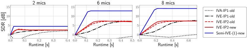
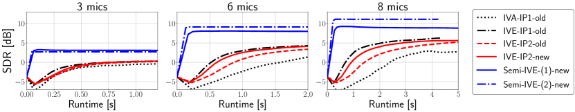
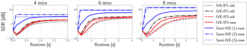
VII-D Experimental results
Figure 1 shows the SDR performance of each algorithm as a function of the runtime, and Table II presents the realtime factor (RTF) of the algorithms when the number of iterations is set to 50 for all the algorithms. These results were obtained by running the algorithms on a PC with Intel(R) Core(TM) i7-7820X CPU @ 3.60GHz using a single thread.
VII-D1 Effectiveness of IVE-IP2-new for extracting unique target source ()
In Fig. 1(a), IVE-IP2-new showed faster convergence than the conventional algorithms while achieving a similar SDR performance. Interestingly, the full-blind IVE algorithms in the cases produced rather better SDRs than the informed Semi-IVE--new in the case. This result motivates us to use more microphones at the expense of increased runtime. As desired, these increased runtime of the IVE algorithms, especially the proposed IVE-IP2-new, was shown to be very small compared to IVA-IP1-old.
VII-D2 Effectiveness of IVE-IP2-new compared to IVE-IP2-old
From Fig. 1 and Table II, it can be confirmed for that the computational cost of the proposed IVE-IP2-new is consistently smaller than IVE-IP2-old while maintaining its separation performance, which shows the effectiveness of IVE-IP2-new. On the other hand, if is small, IVE-IP2-new gave almost the same performance as IVE-IP2-old.
VII-D3 Comparison of IVA-IP1-old, IVE-IP1-old, and IVE-IP2-new
If (Fig. 1(a)), the proposed IVE-IP2-new gave the fastest convergence among other blind algorithms, which clearly shows the superiority of IVE-IP2-new. On the other hand, if (Fig. 1(b)–(c)), the convergence of IVE-IP2-new is slower than that of IVE-IP1-old, mainly because the computational cost per iteration of IVE-IP2-new exceedes that of IVE-IP1-old (see Table II). Therefore, IVE-IP1-old is still important when extracting more than two sources.
VII-D4 Effectiveness of Semi-IVE--new
In Fig. 1, the proposed Semi-IVE algorithms naturally outperformed all of the full-blind IVA and IVE algorithms. Surprisingly, when the transfer functions are given a priori (and ), the Semi-IVE algorithms (Semi-IVE--new if and Semi-IVE--new if ) achieved comparable or sometimes better performance than Semi-IVE--new. The convergence of Semi-IVE--new with was also extremely fast. These results clearly show the effectiveness of the proposed Semi-IVE algorithms.
VIII Concluding remarks
We presented two new efficient BCD algorithms for IVE: (i) IVE-IP2, which extracts all the super-Gaussian sources from a linear mixture in a fully blind manner, and (ii) Semi-IVE, which improves IVE-IP2 in the semiblind scenario in which the transfer functions for several super-Gaussian sources are available as prior knowledge. We also argued that the conventional IVE that relies on the orthogonal constraint (IVE-OC) can be interpreted as BCD for IVE (IVE-IP1). Due to the stationary Gaussian noise assumption, these BCD (or IP) algorithms can skip most of the optimization of the filters for separating the noise components, which plays a central role for achieving a low computational cost of optimization.
Our numerical experiment, which extracts speech signals from their noisy reverberant mixture, showed that when or given at least transfer functions in a semiblind case, the proposed IVE-IP2 and Semi-IVE resulted in significantly faster convergence compared to the conventional algorithms, where is the number of the target-source signals. The new IVE-IP2 consistently speeded up the old IVE-IP2, and the conventional IVE-IP1 remains important for extracting multiple sources.
Appendix A
We prepare several propositions that are needed to rigorously develop the algorithms in Sections IV and V.
Proposition 5 below gives an inequality which is the basis of the MM algorithm for AuxICA [29], AuxIVA [30], and (the auxiliary-function-based) IVE.
Proposition 5 (See [29, Theorem 1]).
Let be differentiable and satisfy that is nonincreasing on . Then, for arbitrary , it holds that
| (92) |
The inequality holds with equality if .
To give a proof of Propositions 2, 3, and 4, we need the following proposition that provides a sufficient condition for the existence of globally optimal solutions.
Proposition 6.
Suppose and . Let be full column rank. The function with respect to , defined by
is lower bounded and attains its minimum at some .
Proof.
Proposition 7 below gives a useful expression of . The same statement for in Proposition 7 can be found in [61], and we here extend it for general .
Proposition 7.
Let and
Then, holds.
Proof.
The orthogonal projection onto is given by . Then, it holds that
where we use in the second equality. ∎
Appendix B Proof of Proposition 3
Proof.
The proof is very similar to that of [26, Theorem 3]. By Proposition 6, problem (45) has global optimal solutions, and they satisfy the stationary conditions (35)–(36). In Eqs. (35)–(36), the first rows except for the th row is linear with respect to and , and so they can be solved as
| (93) | ||||||
| (94) |
where and for are defined by (48)–(49), and and are free variables (the roles of and will be clear below). Substituting (93)–(94) into the objective function , we have
| (95) |
where .
Now, let us consider minimizing with respect to and . In (95), the term can be simplified as
Here, we used twice in the second equality. Hence, by applying Proposition 2, attains its minimum when
| (96) | ||||
| (97) | ||||
| (98) |
where in (98) denotes the largest generalized eigenvalue. Because (97)–(98) are equivalent to (51)–(52) through and , a global optimal solution for (45) can be obtained by
as we desired. ∎
References
- [1] P. Comon and C. Jutten, Handbook of Blind Source Separation: Independent component analysis and applications. Academic press, 2010.
- [2] A. Cichocki and S. Amari, Adaptive blind signal and image processing: learning algorithms and applications. John Wiley & Sons, 2002.
- [3] T.-W. Lee, “Independent component analysis,” in Independent component analysis. Springer, 1998, pp. 27–66.
- [4] J. V. Stone, Independent component analysis: a tutorial introduction. MIT press, 2004.
- [5] T. Kim, H. T. Attias, S.-Y. Lee, and T.-W. Lee, “Blind source separation exploiting higher-order frequency dependencies,” IEEE Trans. Audio, Speech, Language Process., vol. 15, no. 1, pp. 70–79, 2007.
- [6] A. Hiroe, “Solution of permutation problem in frequency domain ICA, using multivariate probability density functions,” in Proc. ICA, 2006, pp. 601–608.
- [7] Y.-O. Li, T. Adali, W. Wang, and V. D. Calhoun, “Joint blind source separation by multiset canonical correlation analysis,” IEEE Trans. Signal Process., vol. 57, no. 10, pp. 3918–3929, 2009.
- [8] X.-L. Li, T. Adalı, and M. Anderson, “Joint blind source separation by generalized joint diagonalization of cumulant matrices,” Signal Processing, vol. 91, no. 10, pp. 2314–2322, 2011.
- [9] M. Anderson, T. Adali, and X.-L. Li, “Joint blind source separation with multivariate Gaussian model: Algorithms and performance analysis,” IEEE Trans. Signal Process., vol. 60, no. 4, pp. 1672–1683, 2011.
- [10] J. H. Friedman and J. W. Tukey, “A projection pursuit algorithm for exploratory data analysis,” IEEE Trans. Comput., vol. 100, no. 9, pp. 881–890, 1974.
- [11] P. J. Huber, “Projection pursuit,” The annals of Statistics, pp. 435–475, 1985.
- [12] J. H. Friedman, “Exploratory projection pursuit,” Journal of the American statistical association, vol. 82, no. 397, pp. 249–266, 1987.
- [13] J.-F. Cardoso and A. Souloumiac, “Blind beamforming for non-Gaussian signals,” in IEE proceedings F (radar and signal processing), vol. 140, no. 6, 1993, pp. 362–370.
- [14] N. Delfosse and P. Loubaton, “Adaptive blind separation of independent sources: A deflation approach,” Signal processing, vol. 45, no. 1, pp. 59–83, 1995.
- [15] S. A. Cruces-Alvarez, A. Cichocki, and S. Amari, “From blind signal extraction to blind instantaneous signal separation: Criteria, algorithms, and stability,” IEEE Trans. Neural Netw., vol. 15, no. 4, pp. 859–873, 2004.
- [16] S. Amari and A. Cichocki, “Adaptive blind signal processing-neural network approaches,” Proceedings of the IEEE, vol. 86, no. 10, pp. 2026–2048, 1998.
- [17] A. Hyvärinen and E. Oja, “A fast fixed-point algorithm for independent component analysis,” Neural Comput., vol. 9, no. 7, pp. 1483–1492, 1997.
- [18] A. Hyvarinen, “Fast and robust fixed-point algorithms for independent component analysis,” IEEE Trans. Neural Netw., vol. 10, no. 3, pp. 626–634, 1999.
- [19] E. Oja and Z. Yuan, “The FastICA algorithm revisited: Convergence analysis,” IEEE Trans. Neural Netw., vol. 17, no. 6, pp. 1370–1381, 2006.
- [20] T. Wei, “A convergence and asymptotic analysis of the generalized symmetric FastICA algorithm,” IEEE Transl. Signal Process., vol. 63, no. 24, pp. 6445–6458, 2015.
- [21] Z. Koldovský and P. Tichavský, “Gradient algorithms for complex non-Gaussian independent component/vector extraction, question of convergence,” IEEE Trans. Signal Process., vol. 67, no. 4, pp. 1050–1064, 2018.
- [22] Z. Koldovský, P. Tichavský, and V. Kautský, “Orthogonally constrained independent component extraction: Blind MPDR beamforming,” in Proc. EUSIPCO, 2017, pp. 1155–1159.
- [23] J. Janský, J. Málek, J. Čmejla, T. Kounovský, Z. Koldovský, and J. Žd’ánský, “Adaptive blind audio source extraction supervised by dominant speaker identification using x-vectors,” in Proc. ICASSP, 2020, pp. 676–680.
- [24] R. Scheibler and N. Ono, “Independent vector analysis with more microphones than sources,” in Proc. WASPAA, 2019, pp. 185–189.
- [25] ——, “Fast independent vector extraction by iterative SINR maximization,” in Proc. ICASSP, 2020, pp. 601–605.
- [26] ——, “MM algorithms for joint independent subspace analysis with application to blind single and multi-source extraction,” arXiv:2004.03926v1, 2020.
- [27] R. Ikeshita, T. Nakatani, and S. Araki, “Overdetermined independent vector analysis,” in Proc. ICASSP, 2020, pp. 591–595.
- [28] K. Lange, MM optimization algorithms. SIAM, 2016, vol. 147.
- [29] N. Ono and S. Miyabe, “Auxiliary-function-based independent component analysis for super-Gaussian sources,” in Proc. LVA/ICA, 2010, pp. 165–172.
- [30] N. Ono, “Stable and fast update rules for independent vector analysis based on auxiliary function technique,” in Proc. WASPAA, 2011, pp. 189–192.
- [31] ——, “Fast stereo independent vector analysis and its implementation on mobile phone,” in Proc. IWAENC, 2012, pp. 1–4.
- [32] ——, “Fast algorithm for independent component/vector/low-rank matrix analysis with three or more sources,” in Proc. ASJ Spring Meeting, 2018, (in Japanese).
- [33] D.-T. Pham and J.-F. Cardoso, “Blind separation of instantaneous mixtures of nonstationary sources,” IEEE Trans. Signal Process., vol. 49, no. 9, pp. 1837–1848, 2001.
- [34] S. Dégerine and A. Zaïdi, “Separation of an instantaneous mixture of Gaussian autoregressive sources by the exact maximum likelihood approach,” IEEE Trans. Signal Process., vol. 52, no. 6, pp. 1499–1512, 2004.
- [35] ——, “Determinant maximization of a nonsymmetric matrix with quadratic constraints,” SIAM J. Optim., vol. 17, no. 4, pp. 997–1014, 2006.
- [36] A. Yeredor, “On hybrid exact-approximate joint diagonalization,” in Proc. CAMSAP, 2009, pp. 312–315.
- [37] A. Yeredor, B. Song, F. Roemer, and M. Haardt, “A “sequentially drilled” joint congruence (SeDJoCo) transformation with applications in blind source separation and multiuser MIMO systems,” IEEE Trans. Signal Process., vol. 60, no. 6, pp. 2744–2757, 2012.
- [38] P. Tseng, “Convergence of a block coordinate descent method for nondifferentiable minimization,” Journal of optimization theory and applications, vol. 109, no. 3, pp. 475–494, 2001.
- [39] D. Kitamura, N. Ono, H. Sawada, H. Kameoka, and H. Saruwatari, “Determined blind source separation unifying independent vector analysis and nonnegative matrix factorization,” IEEE/ACM Trans. Audio, Speech, Language Process., vol. 24, no. 9, pp. 1622–1637, 2016.
- [40] H. Kameoka, L. Li, S. Inoue, and S. Makino, “Supervised determined source separation with multichannel variational autoencoder,” Neural computation, vol. 31, no. 9, pp. 1891–1914, 2019.
- [41] N. Makishima, S. Mogami, N. Takamune, D. Kitamura, H. Sumino, S. Takamichi, H. Saruwatari, and N. Ono, “Independent deeply learned matrix analysis for determined audio source separation,” IEEE/ACM Trans. Audio, Speech, Language Process., vol. 27, no. 10, pp. 1601–1615, 2019.
- [42] K. Sekiguchi, A. A. Nugraha, Y. Bando, and K. Yoshii, “Fast multichannel source separation based on jointly diagonalizable spatial covariance matrices,” in Proc. EUSIPCO, 2019, pp. 1–5.
- [43] N. Ito and T. Nakatani, “FastMNMF: Joint diagonalization based accelerated algorithms for multichannel nonnegative matrix factorization,” in Proc. ICASSP, 2019, pp. 371–375.
- [44] H. L. Van Trees, Optimum array processing: Part IV of detection, estimation, and modulation theory. John Wiley & Sons, 2004.
- [45] E. Warsitz and R. Haeb-Umbach, “Blind acoustic beamforming based on generalized eigenvalue decomposition,” IEEE Trans. Audio, Speech, Language Process., vol. 15, no. 5, pp. 1529–1539, 2007.
- [46] N. Ito, S. Araki, and T. Nakatani, “Data-driven and physical model-based designs of probabilistic spatial dictionary for online meeting diarization and adaptive beamforming,” in Proc. EUSIPCO, 2017, pp. 1165–1169.
- [47] D. H. Johnson and D. E. Dudgeon, Array signal processing: concepts and techniques. Simon & Schuster, Inc., 1992.
- [48] E. Warsitz and R. Haeb-Umbach, “Blind acoustic beamforming based on generalized eigenvalue decomposition,” IEEE Trans. Audio, Speech, Language Process., vol. 15, no. 5, pp. 1529–1539, 2007.
- [49] A. Khabbazibasmenj, S. A. Vorobyov, and A. Hassanien, “Robust adaptive beamforming based on steering vector estimation with as little as possible prior information,” IEEE Trans. Signal Process., vol. 60, no. 6, pp. 2974–2987, 2012.
- [50] S. A. Vorobyov, “Principles of minimum variance robust adaptive beamforming design,” Signal Processing, vol. 93, no. 12, pp. 3264–3277, 2013.
- [51] E. Gómez, M. Gomez-Viilegas, and J. Marin, “A multivariate generalization of the power exponential family of distributions,” Communications in Statistics-Theory and Methods, vol. 27, no. 3, pp. 589–600, 1998.
- [52] S. Amari, A. Cichocki, and H. H. Yang, “A new learning algorithm for blind signal separation,” in Proc. NIPS, 1996, pp. 757–763.
- [53] J. Nocedal and S. Wright, Numerical optimization. Springer Science & Business Media, 2006.
- [54] R. Ikeshita, N. Ito, T. Nakatani, and H. Sawada, “Independent low-rank matrix analysis with decorrelation learning,” in Proc. WASPAA, 2019, pp. 288–292.
- [55] N. Murata, S. Ikeda, and A. Ziehe, “An approach to blind source separation based on temporal structure of speech signals,” Neurocomputing, vol. 41, no. 1-4, pp. 1–24, 2001.
- [56] E. Vincent, R. Gribonval, and C. Févotte, “Performance measurement in blind audio source separation,” IEEE Trans. Audio, Speech, Language Process., vol. 14, no. 4, pp. 1462–1469, 2006.
- [57] S. Nakamura, K. Hiyane, F. Asano, T. Nishiura, and T. Yamada, “Acoustical sound database in real environments for sound scene understanding and hands-free speech recognition,” in LREC, 2000.
- [58] J. Garofolo, L. Lamel, W. Fisher, J. Fiscus, D. Pallett, N. Dahlgren, and V. Zue, “TIMIT Acoustic-Phonetic Continuous Speech Corpus LDC93S1. Web Download. Philadelphia: Linguistic Data Consortium,” 1993.
- [59] J. Barker, R. Marxer, E. Vincent, and S. Watanabe, “The third ‘CHiME’ speech separation and recognition challenge: Dataset, task and baselines,” in Proc. ASRU, 2015, pp. 504–511.
- [60] K. E. Atkinson, An introduction to numerical analysis. John wiley & sons, 2008.
- [61] T. Nakatani and K. Kinoshita, “Maximum likelihood convolutional beamformer for simultaneous denoising and dereverberation,” in Proc. EUSIPCO, 2019, pp. 1–5.