-jettiness in electroweak high-energy processes
Abstract
We study -jettiness in electroweak processes at extreme high energies, in which the mass of the weak gauge bosons can be regarded as small. The description of the scattering process such as is similar to QCD. The incoming leptons emit initial-state radiation and the resultant particles, highly off-shell, participate in the hard scattering, which are expressed by the beam functions. After the hard scattering, the final-state leptons or leptonic jets are observed, described by the fragmenting jet functions or the jet functions respectively. At present, electroweak processes are prevailed by the processes induced by the strong interaction, but they will be relevant at future colliders at high energy. The main difference between QCD and electroweak processes is that the initial- and final-state particles should appear in the form of hadrons, that is, color singlets in QCD, while there can be weak nonsinglets as well in electroweak interactions. We analyze the factorization theorems for the -jettiness in , and compute the factorized parts to next-to-leading logarithmic accuracy. To simplify the comparison with QCD, we only consider the gauge interaction, and the extension to the Standard Model is straightforward. Put it in a different way, it corresponds to an imaginary world in which colored particles can be observed in QCD, and the richer structure of effective theories is probed. Various nonzero nonsinglet matrix elements are interwoven to produce the factorized results, in contrast to QCD in which there are only contributions from the singlets. Another distinct feature is that the rapidity divergence is prevalent in the contributions from weak nonsinglets due to the different group theory factors between the real and virtual corrections. We verify that the rapidity divergence cancels in all the contributions with a different number of nonsinglet channels. We also consider the renormalization group evolution of each factorized part to resum large logarithms, which are distinct from QCD.
Keywords:
jettiness, electroweak processes, rapidity divergence, resummation1 Introduction
The understanding of high-energy scattering has reached a state of the art with the advent of the effective theories such as soft-collinear effective theory (SCET) Bauer:2000ew ; Bauer:2000yr ; Bauer:2001ct ; Bauer:2001yt . The basic picture to this understanding lies in the following procedure. The partons from the incoming protons, as in Large Hadron Collider, participate in the hard scattering and produce a plethora of final-state particles including hadrons, electroweak gauge bosons, Higgs particles and possibly heavy particles beyond the Standard Model. Quantum chromodynamics (QCD) plays a major role in comprehending collider physics phenomenology because the strong interaction acts in every stage of the scattering process with disparate energy scales.
The essence of disentangling the strong interaction is to construct factorization theorems which decompose the high-energy processes into hard, collinear and soft parts. SCET is the appropriate effective theory of QCD for high-energy processes, in which energetic, collinear particles form jets immersed in the sea of soft particles. In SCET we select the relevant collinear and soft modes and integrate out all the other degrees of freedom. Factorization of high-energy processes can be accomplished in SCET by decoupling the soft interaction from the collinear particles. Subsequently the collinear sectors in different directions do not interact with each other. Depending on the observables of interest, the phase space is divided by the definite properties of the specific modes and the factorization theorem is constructed according to how the modes or the phase spaces are organized. Each mode has its own characteristic scale, and typically there is a hierarchy of such scales. The scattering cross sections or event shape observables are expressed in terms of the logarithms of the ratios of the different energy scales, which necessitates the resummation of the large logarithms. Because each factorized part is governed by a single scale in each phase space, the large logarithms in each sector can be resummed to all orders using the renormalization group (RG) equations.
So far, we have described the factorization of high-energy processes in QCD. Here we change gears to employ SCET in extremely high-energy electroweak processes, in which all the masses of the particles including the weak gauge bosons can be regarded as small. By way of illustration, we consider the process , where denotes arbitrary final states, and the jet denotes the jet which includes the muon in the final state.111From now on, we will write for the jets including muons. If we refer to the muons instead of the muon jets, we will explicitly state it. In order to simplify the situation, we consider only the weak gauge interaction by turning off all the other gauge interactions. Therefore we imagine a world with the weak gauge interaction out of the full gauge interactions of the Standard Model. The extension to the Standard Model is complicated, but straightforward. In the high-energy limit, the incoming electron can be regarded as a collection of the “partons” which consist of leptons, weak gauge bosons. These partons undergo a hard collision and produce final-state energetic particles, along with soft particles.
This scenario may sound rather dull because everything mimics the processes in QCD, and one may wonder what, if any, can be learned from this imaginary world. The most interesting issue in this context is that the weak gauge interaction is not confining. It means that the incoming particles or the outgoing particles do not have to be gauge singlets. This is in contrast to QCD, where all the strongly-interacting particles are produced as color singlets, that is, hadrons. Due to this constraint, various matrix elements of the operators in QCD in, say, the parton distribution functions (PDF) or the jet functions are evaluated only for the color singlet configurations. However, the gauge singlets, as well as the gauge nonsinglets participate in weak high-energy processes. It makes the procedure of the factorization more sophisticated, and requires more care in analyzing the interwoven structure. Put it in a different way, it corresponds to imagining QCD without confinement and ask how the factorization works if there are free quarks and gluons. The underlying hard scattering processes can be traced directly and the measurement of the jets and the properties can be reconstructed explicitly by the constituents without worrying about hadronization.
We sketch electroweak high-energy processes by analogy with QCD. The incoming on-shell “partons” (electrons in our case) possess certain fractions of the energy from the initial particles and they radiate away gauge bosons to be far off-shell. This process is described by the electroweak beam functions. Then the energetic partons undergo a hard scattering and the final-state particles can be observed in terms of individual particles, described by the fragmentation functions, or jets by the jet functions or the fragmenting jet functions (FJF). And the soft interaction is interspersed between the collinear parts. In electroweak high-energy processes, gauge singlets and nonsinglets are involved in all these factorized components, which makes the analysis more intriguing. This study will be relevant in high-energy electron-positron colliders such as CEPC dEnterria:2016sca , ILC Djouadi:2007ik , FCC-ee Abada:2019zxq , and CLIC Charles:2018vfv . Our analysis can be extended to include the production of the Higgs boson, weak gauge bosons and top quarks.
There appear many different energy scales, the energy of the hard scattering , the invariant masses of the initial- and final-states as a typical collinear scale, and the soft scale, and possibly more if we are interested in more differential processes describing event shapes. In addition, the mass of the weak gauge bosons also enters into the picture as a physical mass. In radiative corrections, there are logarithms of the ratios of these scales and we need to resum the large logarithms to all orders. In SCET, the factorization is achieved by dissecting the phase space and devising the modes in that phase space such that the radiative corrections depend on a single scale in each phase space. Then the resummation is obtained by solving the RG equation.
Besides the conventional RG behavior, there is additional rapidity divergence because the phase space is divided into different regions. It is obviously absent in the full theory because there is no separation of the phase space. Therefore it is a good consistency check for an effective theory to see whether the rapidity divergences are cancelled when all the factorized contributions are added. It is one of the goals in this paper to check this point even in the presence of the nonsinglets participating in the scattering.
Though the sum of the rapidity divergences cancels, the rapidity divergence remains in each sector and it affects the RG behavior of the factorized parts. The rapidity divergence has been regulated using diverse methods, such as the use of the Wilson lines off the lightcone collins_2011 , the -regulator Idilbi:2007ff ; Idilbi:2007yi , the analytic regulator Becher:2011dz , the rapidity regulator Chiu:2011qc ; Chiu:2012ir , the exponential regulator Li:2016axz , and the pure rapidity regulator Ebert:2018gsn , etc.. Recently one of us has proposed a consistent scheme of applying rapidity regulators to the soft and collinear sectors Chay:2020jzn . It correctly produces the directional dependence in the soft function, which is essential in our case because there are four different collinear directions involved. The independence of the rapidity scale in the cross section critically depends on the interplay between the collinear and the soft functions.
The dependence on the rapidity scale in each sector becomes highly nontrivial and more interesting when gauge nonsinglets as well as singlets participate in high-energy scattering. First of all, let us describe the rapidity divergence for singlets, which is well understood in QCD. The rapidity divergence appears distinctively in and . In , since collinear and soft particles have different offshellness, there is no overlap in rapidity between these modes, hence no rapidity divergence arises. In other words, the rapidity divergence cancels in each sector. On the other hand, in , where collinear and soft particles have the same offshellness, they overlap near the rapidity boundary. The soft particles with small rapidity cannot perceive the large rapidity region which belongs to collinear sector, causing the rapidity divergence in the soft sector. In the collinear sector, according to our regularization scheme of the rapidity divergence, which will be described in detail, the rapidity divergence arises from the zero-bin subtraction Chiu:2011qc ; Chiu:2012ir . The zero-bin subtraction replaces the spurious rapidity divergence in the naive contribution. It is analogous to the pullup mechanism Manohar:2000kr ; Hoang:2001rr in the dimensional regularization, in which the IR divergence is replaced by the UV divergence. The rapidity divergence may survive in each sector, but their sum cancels. However, the persistent existence of the rapidity divergence in each sector offers additional evolution to complete the resummation.
In weak interaction, the structure of the rapidity divergence is more intricate. For gauge singlets, there is no rapidity divergence as in QCD. For gauge nonsinglets, regardless of or , the rapidity divergence is not cancelled in each sector when the weak charges of the initial or final states are specified. Nor are the Sudakov logarithms. The non-cancellation of the electroweak logarithms is known as the Block-Nordsieck violation in electroweak processes Ciafaloni:2000df ; Ciafaloni:2001vt ; Ciafaloni:2006qu ; Manohar:2014vxa . In contrast, the Sudakov logarithms in QCD cancel from virtual and real contributions in inclusive processes. It yields, for example, the Dokshitzer-Gribov-Lipatov-Altarelli-Parisi (DGLAP) evolution of the PDF. The non-cancellation in weak interaction affects the UV behavior as well as the rapidity behavior. Our result is, in some sense, a manifestation of the non-cancellation in considering the event shape through the jettiness.
In the framework of SCET, it was pointed out in ref. Manohar:2018kfx that the nonsinglet electroweak PDFs possess this property. It is also true for the beam function in the initial state, and for the jet functions, or the FJFs in the final state, and for the soft function. The purposes of this paper are to analyze the structure of the factorization in the weak processes, and to resum large logarithms by probing the structure of the divergences including the rapidity divergence from the nonsinglet contributions.
As a concrete example, we consider an event shape, especially the -jettiness Stewart:2010tn ; Jouttenus:2011wh (in fact, 2-jettiness) in . By considering the jettiness, we can probe the hierarchy of scales in effective theories, and the characteristics of a measurement-dependent factorization can be discussed. In addition, we are interested in the case in which there are four distinct lightlike directions. For this reason, -jettiness is better suited than the beam thrust in the Drell-Yan process Stewart:2010pd or the jet thrust in collisions. In terms of QCD, it corresponds to the -jettiness from the partonic subprocess .
The rest of the paper is organized as follows. In section 2, we explain the -jettiness, and establish the power counting of the relevant momenta and the jettiness to choose the appropriate effective theories. In section 3, we first construct the factorization of the -jettiness in , in which the ingredients of the factorized parts are extracted and defined. The beam functions, the semi-inclusive jet functions, and the soft functions are constructed in the context of with the weak singlet and nonsinglet contributions. Then we scale down to and establish the factorization by probing the relations between the beam function in , and the PDF in , or those between the fragmenting jet functions and the fragmentation functions. In section 4, we examine the source of the rapidity divergence, set up the rapidity regulators in the collinear and the soft sectors and discuss their characteristics.
In section 5, we present the radiative corrections of the collinear parts at next-to-leading order (NLO), which consist of the beam functions, the PDFs, the jet functions, the fragmentation functions and the FJFs. In section 6, the hard functions are collected for the process with the left-handed electron and muon doublets, and the hard anomalous dimension matrix is presented. The soft functions are analyzed in section 7, which are expressed in terms of the matrices in weak-charge space. In section 8, we combine all the factorized parts to show the RG evolution of the -jettiness, and we conclude in section 9. Long technical calculations are relegated to appendices. In appendix A, we list the Laplace transforms of the distributions. In appendices B and C, we present how to obtain the collinear functions and the matching coefficients in the limit of small . In appendix D, we illustrate the color matrices for the soft functions at tree level, and we show that there is no mixing at one loop for the soft functions with four nonsinglets.
2 SCET setup for the jettiness in
We consider the -jettiness222We keep using the terminology -jettiness, bearing in mind that we actually consider the 2-jettiness in our case., which is defined as Stewart:2010tn ; Jouttenus:2011wh
| (1) |
where runs over 1, 2 for the beams, and for the final-state jets. Here are the reference momenta of the beams and the jets with the normalization factors , and are the momenta of all the measured particles in the final state.
| (2) |
where are the momentum fractions of the beams. Here and are lightcone vectors for the beams, which are aligned to the direction, , and are the lightcone vectors specifying the jet directions. Typically we write the lightlike vectors as , , where the unit vector denotes the direction of the spatial momentum . The -jettiness in eq. (1) can also be expressed in terms of some arbitrary hard scales instead of the normalization factor .
In references Jouttenus:2011wh ; Bertolini:2017efs , the authors have considered the differential distribution with respect to the individual jettiness, which is defined as
| (3) |
Here we consider the total -jettiness , which is given by .
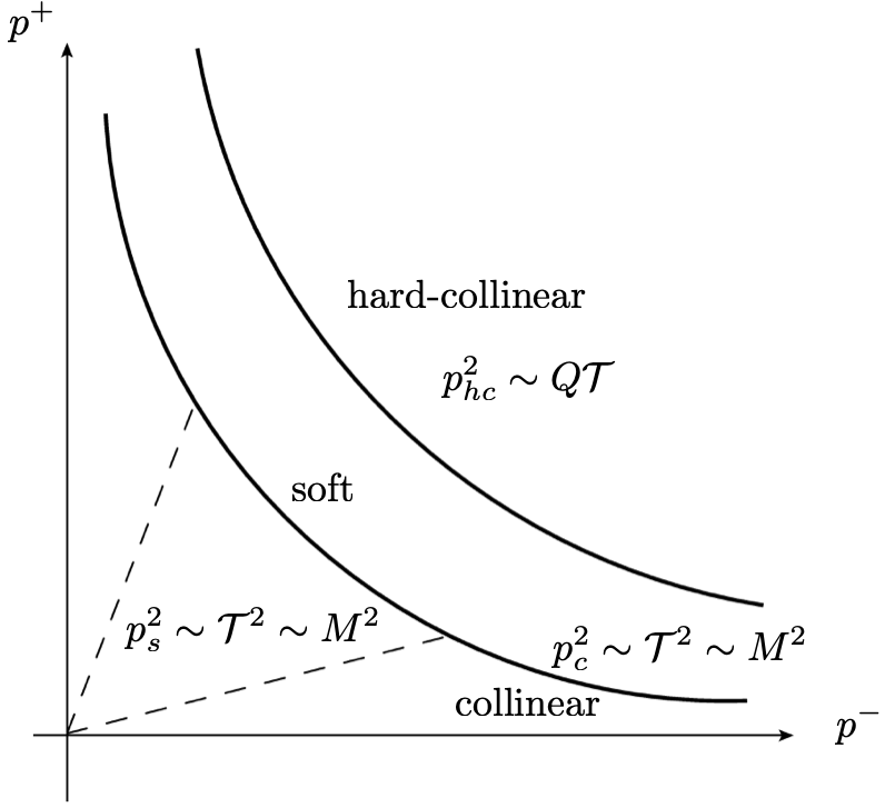
For , SCET can be applied to the process , but we should determine which effective theories are to be employed, depending on the hierarchy of the scales in the collinear and soft momenta and the magnitude of the jettiness. The -collinear momentum scales as , where is the small parameter in SCET. We can consider either , or continue down to , depending on the power counting of the soft momentum.
In , the ultrasoft (usoft) momentum scales as , while the soft momentum in scales as . The gauge boson mass is another mass scale which enters into the system. When the usoft or the soft gauge bosons are on their mass shell, , it implies that the gauge boson mass is power counted as in , and in .
The scale of the -jettiness from eq. (1), is extracted from the lightcone component . Note, however, that the magnitudes of for the collinear and the usoft momenta in are comparable to each other, hence the contribution to the -jettiness comes both from the collinear and the usoft sectors. On the other hand, the magnitude of for the collinear momentum is much smaller than that for the soft momentum in . In this case, the contribution to the -jettiness comes only from the soft sector. Therefore we expect that the structure of the factorization takes different forms in and in .
In , the hierarchy of the scales is given as . The relevant modes scale as
| (4) |
The -jettiness probes the scale of order , hence both the collinear and the usoft parts contribute to the -jettiness.
If we consider the kinematical situation in which , the framework of suffices to describe the -jettiness. However, we would like to include another kinematical case, in which the jet becomes narrower, and we reach the region . Then the plus component does not contribute to the jettiness. However, there remains large logarithms associated with , which should be resummed. This can be achieved by going from to through the matching. The beam functions and the jet functions in have virtuality , and we need a second stage of matching to separate these scales. And the ultrasoft function is scaled down to the soft function, which develops the rapidity divergence. These necessitate the use of .
In , the hierarchy of scales is given by . The hard-collinear, collinear and soft modes scale as
| (5) |
In fact, the hard-collinear modes are not the dynamical degrees of freedom in , but these are the modes from to be integrated out to obtain . The -jettiness probes the scale of order , and the collinear contribution with does not contribute to the jettiness. This is also recognized in ref. Lustermans:2019plv in a different context of measuring the transverse momentum and the 0-jettiness .
We first describe in order to set up the elements of the factorization. In order to obtain , the hard-collinear modes, which are previously collinear modes in , are integrated out to reach the collinear modes in . Note that the scaling of the usoft momentum in , and the soft momentum in remain the same, but the small parameter , responsible for the power counting, is rescaled from to . We present the results in both cases.
3 Factorization for the -jettiness
3.1 :
The procedure of obtaining the effective operators by integrating out the degrees of freedom of order with their Wilson coefficients was previously studied extensively in constructing the weak effective Hamiltonian with the QCD radiative corrections Buchalla:1995vs . We follow the same technique, and the Wilson coefficients for the operators are obtained by matching the full theory onto SCET at any fixed order. The four-lepton operators for the process in SCET are given as333In ref. Manohar:2018kfx , other four-fermion operators are listed for neutrino scattering .
| (6) |
at leading order in . We label the incoming leptons as 1 and 2, and the outgoing leptons as 3 and 4. The index refers to the weak charge ( for the nonsinglet and for the singlet). At tree level, is obtained by the exchange of a gauge boson, which leads to the matching coefficient
| (7) |
where the incoming momenta are and for the weak doublets and with . The matching coefficient for begins at order . Here we can utilize the results of the corresponding four-quark operators in QCD for at NLO, and the Wilson coefficients can be read off from those in QCD in ref. Kelley:2010fn by adjusting the group theory factors for . In constructing the Wilson coefficients for our process, note that only the left-handed doublets participate in the scattering. The effective Lagrangian for the leptonic high-energy scattering can be written as
| (8) |
The fields in the operators are now expressed in terms of the collinear fields in SCET. We refer to refs. Bauer:2000ew ; Bauer:2000yr ; Bauer:2001ct ; Bauer:2001yt for the detailed formulation of SCET, and here we collect the necessary ingredients to express the operators in SCET. We introduce a lightcone vector , and its conjugate light-cone vector such that and . A four-vector can be decomposed as , and the -collinear momentum scales as , where is a small parameter in SCET. The usoft momentum scales as .
The collinear operators, which are invariant under collinear gauge transformations, are constructed in terms of the product of the fields and the Wilson lines. The basic building blocks for the lepton and the gauge bosons are defined as
| (9) |
where is the covariant derivative. The collinear Wilson line is given as
| (10) |
where P denotes the path ordering along the integration path.
At leading order in SCET, the interactions of soft gauge bosons with collinear fields exponentiate to form eikonal soft Wilson lines444When no confusion arises, we refer to the usoft momentum as the soft momentum.. The soft gauge bosons are decoupled by the field redefinition Bauer:2001yt
| (11) |
In this paper we use the fields after the decoupling and we drop the superscript (0) for simplicity. Here is the soft Wilson line in the fundamental representation
| (12) |
Employing SCET, the operators in eq. (6) are written as
| (13) |
The differential cross section for the 2-jettiness is given by Bauer:2008jx
| (14) |
where represents the initial state, denotes the final state, and the sum over includes a sum over states with the appropriate phase space. The function computes the value of the jettiness for the final state . In SCET, the final states consist of the collinear states in the directions () and the soft states . Since the -collinear particles do not interact with each other, and the soft particles are decoupled from the collinear sectors by the redefinition in eq. (11), the final states in the Hilbert space can be expressed in terms of the tensor product of the collinear states and the soft states as
| (15) |
The factorization in SCET is established in the scattering cross section, that is, at the amplitude-squared level, instead of at the amplitude level, as shown in eq. (14). Therefore we need to factorize the product of the operators , which will be reorganized in terms of the collinear operators in each collinear direction along with the soft Wilson lines, and it will be implemented in eq. (14) to express the factorized result for the -jettiness. The product of the operators is given as
| (16) |
We rewrite the product by grouping the fields in respective collinear directions, and use the relation Manohar:2018kfx
| (17) |
where , are the gauge indices, , are the Dirac indices, and . To make the notation concise, we have extended the index to 0 such that
| (18) |
with and are the gauge generators for . We keep as it is for the gauge interaction, and the Casimir invariants are denoted by and . For the gauge group, we put .
After some manipulation, eq. (3.1) can be written as
| (19) |
Here the coefficient will be absorbed into the hard function. In order to construct the expression for the jettiness, all the collinear and the soft parts should be organized in such a way that the contribution to the jettiness from each part becomes manifest.
The -jettiness (the 2-jettiness here) can be expressed in terms of the matrix elements for each collinear part and the soft part, which is schematically expressed as
| (20) |
Eq. (3.1) is unavoidably complicated due to the presence of the gauge indices, compared to the corresponding expression in QCD, in which there are only singlet contributions.
The matrix elements between the corresponding states in the Hilbert space can be obtained because the collinear currents in different collinear directions and the soft part are decoupled. For example, yields the electron beam function, and when we consider the intermediate states, the projection into the -collinear states is inserted. The matrix element describes the final-state jet and the projection is inserted for the intermediate states. The matrix element for the soft Wilson lines yields the soft function, and the intermediate states consist of . The treatment of the matrix elements is delineated below.
3.1.1 The beam function
The beam functions are obtained by taking the matrix elements of and in eq. (3.1) between the initial states or . For the matrix element of , the coordinate can be expanded around the lightcone coordinate , and the subleading terms can be neglected. Then by writing , , the matrix element can be written as
| (21) |
where for the singlet and () for the nonsinglets. In the second line, the integration of the delta functions, which is equal to the identity, is inserted. The operators extract the corresponding momenta for the annihilated particles. And is translated to the origin using the momentum operator .
The last part in the last eq. (3.1.1) can be manipulated as
| (22) |
using the relation , where the operator in the bracket acts only inside the bracket.
Now we change the variables to , with . Then eq. (3.1.1) is written as
| (23) |
where the electron beam function is defined as
| (24) |
Note that the quantity is the contribution to the jettiness. Similarly, the matrix element for can be written as
| (25) |
where the anti-electron (positron) beam function is defined as
| (26) |
3.1.2 The jet function and the semi-inclusive jet function
The matrix element for can be written, by inserting the identity , and translating to the origin, as
| (27) |
where , and the lepton jet function is defined as
| (28) |
The quantity contributes to the jettiness from the jet function. Here the trace refers to the sum over the Dirac indices and the weak charge indices. The definition of the jet function in eq. (3.1.2) may look different from the conventional one, but it turns out to be the same. Eq. (3.1.2) can be written as
| (29) |
which is the same as eq. (2.30) in ref. Stewart:2010qs except the factor . Note that the QCD jet functions single out the color singlet components by taking the color and spin averages. However, since we are dealing with the left-handed fields with a given weak charge, we do not average over spin and color.
Note that is the inclusive jet function, and the nonsinglet part is zero, because the weak doublets with the opposite weak charges contribute with the opposite sign. It is the reason why there is only the color singlet contribution in QCD. Here we can extend the definition of the jet functions such that the individual nonsinglet contribution can be extracted. And it can be probed by observing a muon and an antimuon in each final jet experimentally. If we are interested in the jet in which, say, a lepton (a muon) is observed, we can define the semi-inclusive jet function as
| (30) |
where the lepton is specified in the final state, noting that the phase space for can be written as
| (31) |
Then the semi-inclusive jet function at tree level is normalized as , where is the projection operator to the given lepton . For example, the projection operator for the muon is given by in the weak interaction, and for the muon neutrino.
The terminology ‘semi-inclusive jet function’ was used in ref. Kang:2016mcy , but it is different from ours. Their definition corresponds to our fragmentation function with the final jet instead of a final lepton. It is called the fragmentation function to a jet (FFJ) in ref. Dai:2016hzf . The relation among the FJF, the semi-inclusive jet function and the fragmentation function will be discussed in section 5.3.
In terms of the semi-inclusive lepton jet function, , with the lepton in the final state, can be written as
| (32) |
In a similar way, the collinear matrix element, can be written as
| (33) |
where the semi-inclusive antilepton jet function is given as
| (34) |
The fragmentation function or the FJF will be discussed later.
3.1.3 The soft function
The soft matrix elements from eq. (3.1) are written as
| (35) |
where is given by
| (36) | ||||
Note that we have reshuffled the Wilson lines such that those with the coordinate are moved to the left.
The exponential factor in eq. (3.1.3) disappears by appropriate reparameterization transformations Ellis:2010rwa , and eq. (3.1.3) can be written as , where the soft function for the 2-jettiness is defined as
| (37) |
In this form, the virtual contribution comes from the contraction of the soft Wilson lines to the left-hand side or to the right-hand side of the delta function. The real contribution can be obtained by contracting the Wilson lines across the delta function.
3.1.4 Factorized -jettiness in
Combining all these components, the factorized cross section for the 2-jettiness, according to eq. (14), can be written as
| (38) |
After integrating over the coordinate , the exponential factors in eqs. (3.1.1), (25), (32) and (33) yield the delta function, responsible for the momentum conservation. Note that the last delta function in eq. (3.1.4) corresponds to in eq. (14). The corresponding factorization formula for the -jettiness in QCD in the framework of SCET is presented in refs. Stewart:2009yx ; Stewart:2010tn , and this result is an extension including the nonsinglet contributions.
The Mandelstam variables , , are given by , , , where are the partonic momenta. In terms of , is given by We set the hard coefficients as
| (39) |
where the Wilson coefficients are defined as . The phase space is denoted as , which is given by
| (40) |
At tree level, the jet function is proportional to , and when combined with , it gives , which is the phase space for the final-state particle .
3.2 :
In , the soft momentum scales as , while the -collinear momentum scales as . Therefore the small component does not contribute to the jettiness, and the factorized form of the 2-jettiness in Eq. (3.1.4) should be changed. If we naively employed the PDFs and the fragmentation functions instead of the beam functions and the jet functions, there would be no contribution to the jettiness from these collinear functions Lustermans:2019plv . Schematically, the 2-jettiness in might be written as
| (41) |
where the phase space and the integration with respect to other variables are omitted. The imminent problem in this formulation is that the sum of the anomalous dimensions does not cancel. Here the soft anomalous dimension depends on the jettiness . (This will be explicitly shown later.) But, if we use the factorization of the form in eq. (41), there is no dependence of the anomalous dimensions on the jettiness in collinear functions. As a result, the total sum of the anomalous dimensions does not cancel.
Therefore, care must be taken in obtaining from . In fact, the collinear modes in , scaling as , are integrated out to obtain . We call the collinear modes in as the hard-collinear modes in . In fig. 1, the hyperbolas for the collinear and soft modes and for the hard-collinear modes are shown. By integrating out the hard-collinear modes, we obtain the corresponding matching coefficients between and .
The relation between the beam function and the PDF can be obtained by the operator product expansion (OPE) of the relevant operators. Let us consider the operators
| (42) |
of which the matrix elements yield the beam function in eq. (24), and
| (43) |
of which the matrix elements yield the PDFs555For SU() with , there should be an additional nonsiglet gauge boson operator , where is replaced by the structure constant . It is also true in eq. (3.2) below.. [See eq. (73) below.]
Using the OPE in the limit , we can expand the operators in terms of a sum of the operators Stewart:2010qs
| (44) |
Eq. (44) shows the matching relation between the operators in , and the operators in , where are the corresponding Wilson coefficients. When we take the electron matrix element of eq. (44), we obtain the OPE for the beam functions, with ,
| (45) |
We can establish the relation between the semi-inclusive jet functions in , and the fragmentation functions in in the same way. Let us consider the operators in
| (46) |
which yield the semi-inclusive jet functions, and the operators in
| (47) |
where we will choose the frame such that the transverse momentum is zero in taking the matrix elements. We employ the OPE in the limit to expand the operators in terms of the operators as
| (48) |
This equation shows the matching relation between in , and in , where are the corresponding matching coefficients. In order to obtain the relation between the semi-inclusive jet function in , and the fragmentation function in , we take the vacuum expectation values, but with the state included in the intermediate states. The result is written as
| (49) |
In addition, the soft Wilson lines are obtained by integrating out the offshell modes when the soft gauge particles are emitted from the collinear source, which are given by
| (50) |
where is the soft gauge field. As a result, the soft Wilson line in is replaced by , which is the rescaled version in .
With these ingredients, the cross section for the 2-jettiness in is written as
| (51) |
In addition to the contribution of the soft function to the 2-jettiness, note that there are contributions from the hard-collinear contributions. The expression in eq. (3.2) also conforms to the consistent RG behavior of the 2-jettiness. That is, the sum of the anomalous dimensions of all the factorized parts should be zero so that the 2-jettiness is independent of the factorization scale. It cancels only when we use eq. (3.2).
We will present the matching coefficients and explicitly, but a practical way to calculate the collinear parts in is to compute the beam functions and the jet functions using the power counting in , and perform the soft zero-bin subtraction. That is, we compute the combination of the matching coefficients and the PDF or the fragmentation functions together in , which are equivalent to the computation of the beam functions and the FJF in .
The factorization for the -jettiness is established both in and . However, there is an important caveat that Glauber exchange between spectator partons may violate factorization when the weak charges of the final states are specified Baumgart:2018ntv . The possible breakdown of the factorization may start at order of the magnitude , and it is due to the fact that the group-theory factors for the exchange of two Glauber gauge bosons in different configurations across the unitarity cuts are different and the overall effects do not cancel. This should be considered seriously in ascertaining the factorization in electroweak interaction, but it is beyond the scope of this paper, and will not be considered here.
4 Treatment of rapidity divergence
In SCET, the rapidity divergence shows up because the collinear and the soft modes reside in disparate phase spaces. When these modes have the same invariant mass, they are distinguished by their rapidities. The rapidity divergence appears without regard to the UV and IR divergences, hence it has to be regulated independently. As mentioned in section 1, there are various methods to regulate the rapidity divergence collins_2011 ; Idilbi:2007ff ; Idilbi:2007yi ; Becher:2011dz ; Chiu:2011qc ; Chiu:2012ir ; Li:2016axz ; Ebert:2018gsn . In ref. Chay:2020jzn , one of the authors has constructed consistent rapidity regulators both for the collinear and the soft sectors, and we use this prescription here.
The essential idea is to attach a regulator of the form for the -collinear field, where the rapidity divergence arises. And the rapidity regulator in the soft sector should have the same form as that of the collinear rapidity regulator because we track the same source of the radiation, which causes the rapidity divergence, as in the collinear sector. However, it can be written in such a way to conform to the expression of the soft Wilson line. As an example, let us specify the rapidity regulator for the collinear current with , which is not necessarily back-to-back. The collinear and soft Wilson lines and are inserted to make the current collinear and soft gauge invariant. For the collinear Wilson line and the soft Wilson line , the modified Wilson lines with the rapidity regulator are given as
| (52) |
where is the operator extracting the momentum. The remaining Wilson lines and can be obtained by switching and . The point in selecting the rapidity regulator is to trace the same emitted gauge bosons both in the collinear and the soft sectors, which are eikonalized to produce the Wilson lines. Note that the rapidity divergences from and have the same origin because the collinear and soft gauge bosons are emitted from the -collinear quark for both of the Wilson lines. For the soft momentum , in the limit where the rapidity divergence occurs in the soft sector, it becomes and the soft rapidity regulator approaches
| (53) |
which has the same form as the collinear rapidity regulator for . Another pair possessing the same source of rapidity divergence is and . Tracking the same source of the emission of gauge bosons in the soft sector gives the correct directional dependence in the soft anomalous dimensions, in the sense that they cancel the total anomalous dimensions when combined with other factorized parts Bertolini:2017efs .
The source of the rapidity divergence can be understood as follows: For the soft modes with small rapidities, they cannot recognize the region with large rapidity, in which the collinear modes reside. But these collinear modes are obtained by traversing the boundary from the soft sector to the collinear sector. Technically, with the momentum , the rapidity divergence arises when or approaches infinity while is fixed. Therefore we modify the region with large rapidity such that the rapidity divergence can be extracted.
On the other hand, for the -collinear modes, cannot approach infinity in the real contribution because it cannot exceed the large scale . Therefore, in our choice of the rapidity regulators, there is no rapidity divergence in the naive collinear contribution, though there appears the divergence associated with the region . However, the true collinear contribution is obtained by performing the zero-bin subtraction Chiu:2011qc ; Chiu:2012ir in which the collinear contribution in the soft limit is removed to avoid double counting. The zero-bin subtraction can be regarded as the matching between the collinear part with large rapidity and the soft part with small rapidity when the soft part is obtained by integrating out the region with large rapidity.
The divergence in the collinear part as with fixed is cancelled by the zero-bin subtraction in analogy to the cancellation of the IR divergence in matching. Note that the rapidity divergence from the collinear sector has the opposite sign compared to the rapidity divergence in the soft sector. It is the reason why the rapidity divergences cancel when the collinear and the soft sectors are combined. It is consistent with the fact that the full QCD does not have any rapidity divergence since there is no such kinematic constraint, separating the collinear and the soft modes. However, the structure of rapidity divergence and its evolution in each sector sheds light on the intricate nature of the theory.
In electroweak interaction, in which the weak nonsinglets can appear in each factorized part, the behavior of the rapidity divergence is strikingly different from QCD. In collinear quantities such as the jet function, and the FJF, etc., the rapidity divergence cancels for the gauge singlets in each function. Technically, this happens due to the fact that the real and virtual contributions to the rapidity divergence are equal, but with the opposite sign. For gauge nonsinglets, the group theory factors are different for real and virtual contributions, hence producing nontrivial rapidity divergence in each sector. We will present the resummed result at next-to-leading logarithmic (NLL) order for the 2-jettiness in , evolving both under the renormalization scale and the rapidity scale. The cancellation of the rapidity divergence when all the contributions are added becomes more sophisticated. But the non-cancellation of the rapidity divergence in each sector for the gauge singlets induces the additional evolution with respect to the rapidity scale in the process of resummation.
5 Collinear functions
5.1 Beam function and PDF
The beam functions for QCD are defined in refs. Stewart:2009yx ; Stewart:2010qs , and they describe the initial-state radiations from the incoming particles. We can extend them to those for the weak interaction. The singlet and nonsinglet beam functions are defined as the matrix elements with a target electron in our case, which are given as [See eq. (26).]
| (54) |
where and are the weak generators. The beam functions at tree level are given as
| (55) |
where is the projection operator in the weak charge space to project out the electron , because the beam function is initiated by the incoming electron. Otherwise, the nonsinglet beam function vanishes because the contributions from the electron and the electron neutrino cancel. In QCD, since the initial state consists of a color singlet, say, a proton, the color average is performed in the beam function. However it is not true in this case. If we consider the imaginary situation in which the color can be measured in QCD, we should define the beam function with fixed color charges. The beam functions for antileptons can be defined accordingly as
| (56) |
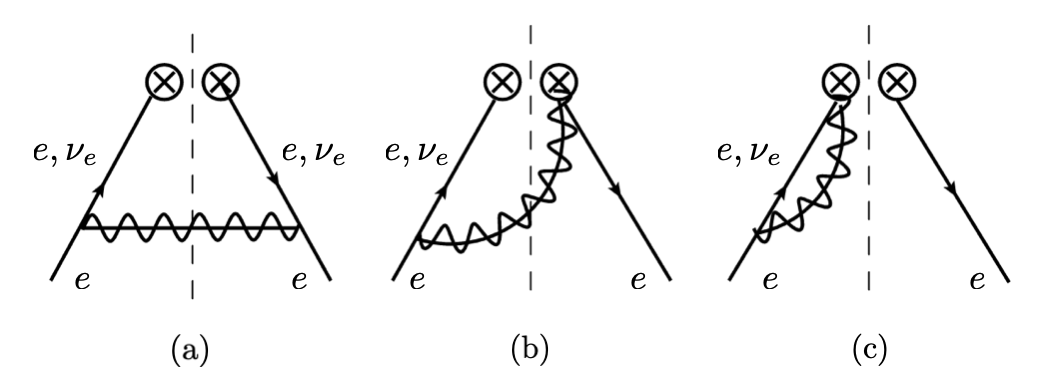
The Feynman diagrams for the beam function at order are shown in figure 2. We choose the reference frame in which the transverse momentum of the incoming particle is zero. Our computational method is different from what was performed in ref. Stewart:2010qs . Here all the massless fermions are on the mass shell with the nonzero gauge boson mass . In our computation, we express the beam functions and the PDFs in terms of the variables and , while we put . Nonzero plays the role of an IR regulator in ref. Stewart:2010qs . In our calculation, the massless fermions are on the mass shell and there is no IR divergence because of the physical nonzero gauge boson mass .
The radiative correction of the singlet beam function at order is different in finite terms from the result in ref. Stewart:2010qs , but the matching coefficients between the beam functions and the PDFs turn out to be the same. However, what is new here is that we include the nonsinglet contributions which show distinct behavior, compared to the singlet contributions. In , since , we take the limit of small in the final result. In , the hard-collinear contribution from the matching coefficients contains , and we also take the small limit.
The contribution of figure 2 (a) apart from the group theory factor is given by
| (57) |
The last result is obtained by taking the small limit. The detailed calculation taking this limit is presented in appendix B. There is no zero-bin contribution for at leading order.
The naive collinear contribution in figure 2 (b), with the momentum of the gauge boson, yields
| (58) |
We put because there is neither UV nor rapidity divergence.
The zero-bin contribution from figure 2 (b), in which the rapidity regulator in eq. (4) is implemented, is given by
| (59) |
where the following relation is used.
| (60) |
The distributions are listed in appendix C.1 Ligeti:2008ac .
By performing the contour integral in the complex -plane, the naive collinear contribution of figure 2 (c) is given as
| (61) |
where . And the zero-bin contribution is given as
| (62) |
The net contribution with the zero-bin subtraction is given as
| (63) |
where the zero-bin contribution is split such that there is no divergence near . Note that the rapidity divergence occurs at large region due to the zero-bin subtraction which cancels the divergence at small from the naive collinear contribution. The result is consistent with ref. Chay:2020jzn . The zero-bin contributions can be computed for the jet functions, FJF, etc. in the same spirit. The wavefunction renormalization and the residue at one loop are given by
| (64) |
We express the singlet and nonsinglet beam functions and in terms of and by extracting and separating the group theory factors as666We will also separate the group theory factors and express the singlet and nonsinglet functions in a similar way for the PDFs [eq. (76)], the matching coefficients between the beam functions and the PDFs [eq. (81)], the jet functions [eq. (84)], the FJFs [eq. (5.3)], and the matching coefficients between the fragmentation functions and the FJFs [eq. (101)].
| (65) |
The bare beam functions and are given at NLO as
| (66) | ||||
Here the splitting function for is the same as the quark splitting function , and is given by
| (67) |
Note that the group theory factors for the real emission (, ) and for the virtual correction (, and ) are the same for the singlet, while they are different for the nonsinglet. Due to this fact, the rapidity divergence cancels in the singlet, while it does not in the nonsinglet.
The -anomalous dimensions and the -anomalous dimensions of the beam functions are given as
| (68) |
where at NLO.
The 2-jettiness in eqs. (3.1.4) and (3.2) is expressed in terms of the convolution of the collinear and the soft functions, but it is convenient to express it in terms of the Laplace transform because the 2-jettiness is expressed in terms of the products. For the beam function, we make a Laplace transform with respect to the jettiness , which is written as
| (69) |
When we make a Laplace transform of the various collinear functions, each part should contain the same scale, and we choose . Here is an arbitrary scale involved in the Laplace transform. Various distributions appearing in eq. (5.1) are expressed as regular functions in the Laplace transforms. (See appendix A.) As we will show later, the evolution of the jettiness is independent of the factorization scale , as well as .
The anomalous dimensions of the Laplace-transformed beam functions are given as
| (70) |
To be precise, these anomalous dimensions are those of the beam functions in , but in , they are regarded as the anomalous dimensions of the combination of the matching coefficients and the PDFs. Here is the cusp anomalous dimension Korchemsky:1987wg ; Korchemskaya:1992je , which can be expanded as
| (71) |
with
| (72) |
To NLL accuracy, the cusp anomalous dimension to two loops is needed.
The PDFs are defined in terms of the matrix elements with a target as
| (73) |
and it is normalized at tree level as
| (74) |
The Feynman diagrams for the PDFs at one loop are shown in figure 2. Note that the Feynman diagrams are the same as those for the beam functions, but the measured quantities are different. Including the zero-bin subtractions, the matrix elements apart from the group theory factors are given as
| (75) |
The singlet and nonsinglet PDFs are expressed in terms of and as
| (76) |
where and at NLO are given as
| (77) |
Here the rapidity divergence shows up in the nonsinglet PDF for the same reason as in the beam functions. It coincides with the result in ref. Manohar:2018kfx . The - and -anomalous dimensions of the PDFs are given as
| (78) | ||||
It is noteworthy to compare the distinction between QCD and the weak interaction. The results for the singlets correspond to QCD and there is only a single logarithm in the singlet PDF, and it satisfies the usual DGLAP equation
| (79) |
where is the analog of the splitting function in QCD. On the other hand, the nonsinglet PDF shows the double logarithms due to the mismatch of the real and virtual contributions, along with the rapidity divergence. Due to the double logarithms, the nonsinglet PDF satisfies more complicated RG equations. It happens to all the collinear functions and the soft function, which necessitates the introduction of .
The beam functions are related to the PDFs as
| (80) |
where are the matching coefficients, which describe the collinear initial-state radiation and can be computed perturbatively. Here , are the indices for particle species, and , are the weak indices. The only nonzero matching coefficients are those which are diagonal in weak-charge space, from which the singlet and nonsinglet matching coefficients and are defined as
| (81) |
The matching coefficients for the singlet and for the nonsinglet at NLO are given as
| (82) |
The finite terms in the beam functions and PDFs are different compared to the result in ref. Stewart:2010qs due to the presence of the gauge boson mass , but the matching coefficient is the same. Note that there is no dependence on in the matching coefficients, because they should be independent of the low-energy physics. The matching coefficient for the nonsinglet is new, but interestingly enough, it is proportional to for the singlet.
5.2 Semi-inclusive jet functions
The semi-inclusive jet functions are defined in eq. (3.1.2). The Feynman diagrams at order are shown in Fig. 3. As in computing the beam functions, the final result is obtained by taking the limit of small . All the contributions including the zero-bin contributions without the group theory factors at NLO are given as (See appendix C.1.)
| (83) |
and the wavefunction renormalization and the residue are given by eq. (64). We put , where , and is the jettiness from the jet.
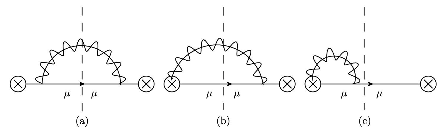
The bare singlet and nonsinglet semi-inclusive jet functions and , which include the lepton in the final state, are given as
| (84) |
where is the projection operator to the lepton (). With the appropriate group theory factors, the bare singlet and the nonsinglet jet functions at NLO are given as
| (85) | ||||
Here again the nonsinglet jet function develops the rapidity divergence.
The anomalous dimensions are given as
| (86) |
The Laplace transforms of the anomalous dimensions with conjugate to the jettiness are given by
| (87) |
which are the same as the anomalous dimensions of the beam functions in eq. (70).
5.3 Fragmentation functions and fragmenting jet functions
The collinear parts pertaining to the final states are described either by the fragmentation functions or by the FJFs. The fragmentation function is used when a single particle is observed with no properties of the jet to be probed. The FJF describes the fragmentation of a parton to another parton within a jet originating from with the measurement of the momentum fraction and the invariant mass of the jet.
The fragmentation function from to the lepton is extended from the definition in QCD Procura:2009vm ; Jain:2011xz to
| (88) |
where is the fraction of the largest lightcone components of the observed lepton originating from . At tree level, the fragmentation functions are normalized as
| (89) |
The matrix elements for the fragmentation functions are the same as those for the PDFs in eq. (5.1), and we will not present them here.
The FJF is defined as
| (90) | ||||
where is the invariant mass of the collinear jet. The small component is the jettiness from the fragmented lepton. The FJF is normalized at tree level as
| (91) |
The relations between the FJF, the semi-inclusive jet functions, and the fragmentation functions can be found by comparing eqs. (3.1.2), (88) and (90). The FJF probes the differential distributions with respect to the invariant mass and the momentum fraction . If we integrate the FJF over all the possible invariant masses, it yields the fragmentation functions which shows the distributions of the momentum fraction of the observed lepton. On the other hand, if we integrate the FJF over the momentum fraction , it yields the semi-inclusive jet function for the lepton in the final state. Therefore the relations can be expressed as
| (92) |
and it is confirmed at order . Our definition of the semi-inclusive (singlet) jet function is different from that in ref. Kang:2016mcy . As explained by the authors in ref. Kang:2016mcy , their semi-inclusive jet function is similar to the fragmentation function. To be exact, it is the fragmentation function, in which the final-state hadron forms a jet. Our semi-inclusive jet function describes the jet mass distribution with the lepton (or the leptonic jet which includes ) in the final state.
In ref. Jain:2011xz , integrating the FJF with an additional factor yields the inclusive jet function . The additional factor of is due to the symmetrization of the final states when all the hadrons in the final state are summed over. However, we refer to the semi-inclusive jet function for the lepton specified in the final state in eq. (92). If we sum over all the final leptons to yield the inclusive jet functions, the additional factor of should be included.
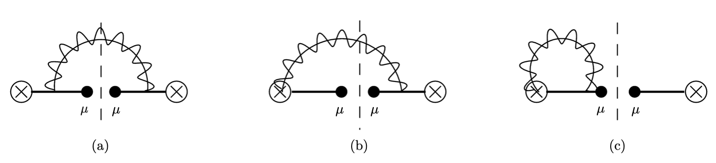
The Feynman diagrams for the fragmentation functions and the FJFs are shown in figure 4. Though we present the same Feynman diagrams for both functions, note that the observed quantities are different. The matrix elements for the FJF without the group theory factors are given at NLO as
| (93) |
Here we also express the matrix elements in the limit of small mass . The detailed derivation of taking the limit is presented in appendix C.2.
The singlet and nonsinglet FJFs are written as
| (94) |
The bare FJFs for the singlet and the nonsinglet at NLO are given as
| (95) | ||||
| (96) | ||||
The singlet FJF in eq. (95) is the same as the result in ref. Jain:2011xz though the individual contributions are different. However, the result for the nonsinglet FJFs is new, and note that the dependence on the rapidity scale remains in the nonsinglet FJFs, while there is none for the singlet FJFs.
The anomalous dimensions are given as
| (97) |
and their Laplace transforms are given by
| (98) |
Because there is a relation between the semi-inclusive jet function and the FJF in eq. (92), the anomalous dimensions of the jet functions and the FJFs are the same. [See eqs. (5.2) and (5.2).]
The matching between the fragmentation function and the FJF are written as
| (99) |
at leading power, where are the matching coefficients. At tree-level, it is given by
| (100) |
If we write
| (101) |
the singlet matching coefficient and the nonsinglet matching coefficient at order are given as
| (102) |
The matching coefficients for the singlet are the same as those in QCD Jain:2011xz . As in the case of the matching coefficients for the beam functions and the PDFs, the new nonsinglet matching coefficient is proportional to the singlet matching coefficient. These matching coefficients do not depend on the gauge boson mass , as in the matching coefficients in eq. (5.1).
6 Hard function
The hard functions are represented by a matrix in the basis of the singlet and nonsinglet operators , so are the soft functions. The hard functions are defined in eq. (39) as , where is the Wilson coefficient of the operators for the process . Here and are electron and muon doublets respectively because the relevant hard processes involve lepton doublets at higher orders. The hard coefficients are determined by matching the results of the full theory onto the effective theory.
We can utilize the results of the hard functions in previous literature. The detailed form of the hard function at one loop for partonic processes can be found in ref. Kelley:2010fn for QCD, and in ref. Chiu:2009mg for electroweak interactions. Since we deal with the left-handed fields, all the right-handed contributions are put to zero.
The Wilson coefficients to order are given by Kelley:2010fn ; Chiu:2009mg
| (103) |
where
| (104) |
The function as a function of the Mandelstam variables is given by
| (105) |
The RG equation for can be written as
| (106) |
where is the anomalous dimension matrix for the Wilson coefficients. Then the RG equation for the hard function is given as
| (107) |
The anomalous dimension matrix is given by Kelley:2010fn ; Chiu:2009mg
| (108) |
where the term compensates the dependence in the leading Wilson coefficients. Here the beta function is given by
| (109) |
The matrix can be written as
| (110) |
where , and . By explicitly computing the color factors Chiu:2009mg , the matrix is written as
| (111) | ||||
with .
7 Soft function
The soft functions for the -jettiness or more general jet observables have been discussed in refs. Jouttenus:2011wh ; Bertolini:2017efs . The authors have considered the differential jettiness, that is, the individual jettiness in the jets. [See eq. (3).] Here we consider the total jettiness which corresponds to the sum of the individual jettiness. The soft function for the jettiness is defined in eq. (3.1.3). Since the calculation was performed in massless cases in these references, they set the virtual contribution to zero since they consist of scaleless integrals. In our scheme with the nonzero gauge boson mass, there is nonzero virtual contribution, and we present the results here.
7.1 Hemisphere soft function
The diagrams for the emission of a gauge boson between the soft Wilson lines and ( and in ) are shown in figure 5, where is the soft Wilson line in the direction. Because , the emission from the soft Wilson lines with vanishes. Figure 5 (a) [figure 5 (b)] denotes the virtual contribution (the real contribution). In computing the total soft function, we include all the possible combinations of and with the appropriate group theory factors. The following calculations are based on the contractions of a gauge boson from the soft Wilson lines and . The additional minus signs when the contractions are performed between and or and are included in the group theory factors.
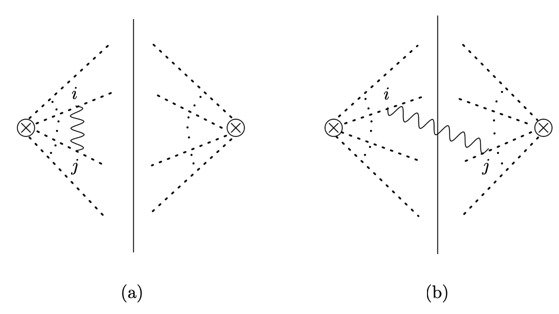
The real contribution is decomposed into the hemisphere and the non-hemisphere parts. Only the hemisphere part involves the divergence, and the non-hemisphere parts are finite Jouttenus:2011wh ; Bertolini:2017efs . Our case is relevant to ref. Jouttenus:2011wh , which corresponds to the case in ref. Bertolini:2017efs . We concentrate on the hemisphere soft function to extract the anomalous dimensions of the -jettiness soft function. The virtual contribution is not affected by the process of choosing the hemisphere functions in the real contribution.
The virtual contribution in figure 5 (a) aside from the group theory factor is written as
| (112) |
where and , and is the rapidity regulator, which can be written at NLO as Chay:2020jzn
| (113) |
Since the integrand in eq. (112) is symmetric under , the contributions from both terms in the rapidity regulator is the same. Here we pick up the first term in the rapidity regulator and multiply two to get the virtual contribution. It is given as
| (114) | ||||
In the third line, we change variables , . Then and are written as , with , with and .
Here we focus on the real part. The imaginary part can be obtained by implementing the prescription for the soft Wilson lines Chay:2004zn . The result can be summarized as follows: The logarithmic term can be expressed in the form , where when and are both incoming or outgoing, and when one is incoming and the other is outgoing. When , the imaginary part is induced.
The real soft contribution without the group theory factor at order is given as
| (115) |
where the function constrains the phase space on the emission of a single gauge boson, from which the hemisphere soft function is to be extracted.
For 2-jettiness, we consider four independent labels , , , and the constraint function is given by
| (116) |
(See ref. Jouttenus:2011wh for 1-jettiness.) In obtaining the second relation, the theta functions in the first term is replaced by
| (117) |
The hemisphere measurement function for the full hemisphere is given by
| (118) |
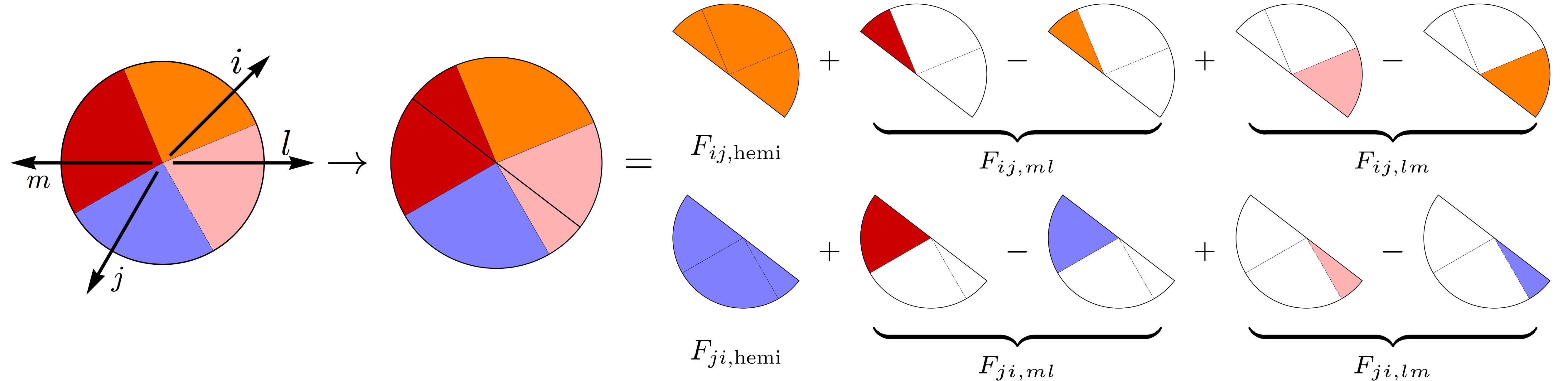
And the non-hemisphere functions are given by
| (119) |
which are the non-hemisphere measurement function for region and respectively. Note that the constraint function is constructed for the gauge boson emitted from the soft Wilson lines and ( and ). The hemisphere function for the and jet directions contains the collinear and the soft divergences. The contribution to the and directions only contains the soft divergence, which is subtracted from the corresponding region of the hemisphere parts. Here we focus on the hemisphere soft functions, from which the anomalous dimensions are obtained. The decomposition of the soft real contribution into the hemisphere functions and the non-hemisphere functions are schematically shown in figure 6. As can be seen in the figure, the soft divergence in the non-hemisphere parts is cancelled by the corresponding subtraction from the hemisphere parts.
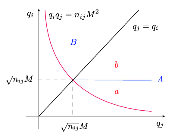
The phase space for the real emission is shown in figure 7, and we compute the real contribution in the phase space , which corresponds to the hemisphere constraint .
The real contribution from the region is given by
| (120) |
We divide the phase space into the region with and the region with , and the integral in the region is given as
| (121) |
where the following relation is used.
| (122) |
The integral in the region is written as
| (123) |
Note that is remains the same when and are switched. Therefore the real contribution is twice because the integration in the region is the same. The real hemisphere contribution is given by
| (124) | ||||
With the virtual contribution in eq. (114) and the real contribution in eq. (124), the hemisphere soft function can be written as
| (125) |
Here we represent the color structure of the soft function in the form , in which the indices represent the presence of the nonsinglets from the originating -th collinear particle ( for the incoming particles, and for the outgoing particles in our convention). For example, the soft color matrix with all the singlets is given by and the soft color matrix with the nonsinglet contributions from 1 and 3 is denoted as , etc.. For the soft color matrix at tree level, see appendix D.1. With these color matrices, the real soft function for the nonsinglets 1 and 3 is written as , where is the soft correction, which is given by eq. (124). Using this convention, the hemisphere soft function from incorporates by putting the generators and for the first and the third indices respectively, and in the second and the fourth indices.
The virtual and real contributions to the and soft anomalous dimensions without the group theory factors are given as
| (126) |
The derivatives of the Laplace-transformed soft parts are given by
| (127) | ||||
| (128) |
It is noteworthy to compare eq. (127) with the results in ref. Manohar:2018kfx , in which the soft anomalous dimensions are given in inclusive cross sections. In ref. Manohar:2018kfx , the virtual and the real contributions at order are the same except the sign, and the -anomalous dimensions depend on . However, in the case of the jettiness in which we give constraints on the phase space in the real emissions, the contribution to the anomalous dimension from the virtual corrections is the same as in ref. Manohar:2018kfx , but the contribution from the real emission is different, especially it is independent of .
Due to this difference, the -jettiness soft function with four nonsinglets does not have mixing in contrast to the inclusive soft function, in which the mixing is induced at one loop. The virtual corrections do not cause mixing, while the mixing is cancelled in the sum of the real contributions because the real soft anomalous dimensions in eq. (127) is independent of . The proof that there is no mixing in the -jettiness soft function with four nonsinglets at one loop is presented in detail in appendix D.2.
7.2 Soft anomalous dimensions
The soft functions are written as matrices in the operator basis. The Laplace transform of the soft function is given as
| (129) |
The RG equation with respect to the renormalization scale for the soft function in Laplace transform is written as
| (130) |
where is the -anomalous dimension matrix. At NLO, eq. (130) is written as
| (131) |
where is the renormalized soft function. The soft anomalous dimensions can be extracted from the requirement that the sum of the anomalous dimensions from all the factorized parts should cancel. The soft anomalous dimension at one loop is given by
| (132) |
where is the anomalous dimensions of the beam functions or the jet functions. The -anomalous dimensions of the soft function with nonsinglets () are given as
| (133) |
where is the matrix in eq. (111) appearing in the hard function. As in the hard function, the imaginary part in the identity matrix does not contribute to the evolution.
The RG equation with respect to the rapidity scale is written as
| (134) |
After color algebra Sjodahl:2012nk , the -soft anomalous dimensions with nonsinglets () are given as
| (135) |
Note that there is no contribution from those with one nonsinglet due to charge conservation.
8 Renormalization group evolution
In order to study the RG evolution, it is convenient to make a Laplace transform of the -jettiness which involves the convolution of the jet, beam and the soft functions in the factorization formulae, eqs. (3.1.4) and (3.2). The convolution becomes the product of the factorized parts with their Laplace transforms. Here we choose , which is the conjugate variable to the jettiness. Then we can take inverse Laplace transform and express the evolutions accordingly Becher:2006mr .
In order to resum large logarithms, the RG evolutions of the factorized functions start from their own characteristic scales to the common factorization scale and the rapidity scale . The characteristic scales are the scales which minimize the logarithms in the factorized functions, and they are give by
| (136) |
where () are the largest collinear components. The characteristic collinear scales (hard-collinear scales in ) apply both to the singlets and the nonsinglets of the collinear functions. The collinear rapidity scale belongs to the nonsinglets. The soft scale applies to both the singlets and the nonsinglets, while the scale belongs to the nonsinglet soft functions.
8.1 Hard function
The anomalous dimension of the hard function is given by eq. (108). The evolution of the hard function from the high-energy scale to the factorization scale is written as
| (137) |
where is the evolution from the identity matrix of the anomalous dimension, and is obtained by the exponentiating the matrix . They can be written as
| (138) |
where
| (139) |
and and are given as
| (140) |
for an arbitrary function . The explicit results of , and are presented at next-to-next-to-leading-logarithmic accuracy in ref. Stewart:2010qs . And is obtained by exponentiating as
| (141) |
8.2 Collinear functions
We present the evolution of the beam functions as a representative of the collinear functions. Since the semi-inclusive jet functions and the FJFs have the same anomalous dimensions as the beam functions, their evolutions can be described in a similar way.
The RG equation with respect to for the singlet beam function is given by
| (142) |
where the -anomalous dimension for the singlet is given by eq. (70). The evolution from the collinear scale to the factorization scale is given by
| (143) |
where the evolution kernel is given by
| (144) |
For the nonsinglet, the and RG equations are given by
| (145) |
where the -anomalous dimensions and the -anomalous dimensions for the nonsinglet are given by eq. (70). The order of the evolutions with respect to and is irrelevant, and here we evolve the beam function with respect to first, and then with respect to . Since the -anomalous dimension contains a large logarithm with , we resum this large logarithm first in expressing the evolution with respect to Chiu:2012ir . Then the evolution is written as
| (146) |
where the -evolution kernel and the -evolution kernel are given by
| (147) | ||||
The anomalous dimensions of the semi-inclusive jet functions in eq. (5.2) are the same as those of the beam functions. Therefore the evolution of the semi-inclusive jet functions is the same as the FJF. However, the largest lightcone component in each -th collinear direction is denoted by , which determines the characteristic collinear scale in each direction. Let us denote the collinear functions as , where it corresponds to the beam functions for and to the semi-inclusive jet functions or the FJFs for . Then the evolution of the collinear functions are written as ()
| (148) |
where the evolution kernels are given as
| (149) |
8.3 Soft function
The and anomalous dimensions for the soft function are given by eqs. (133) and (135) respectively. The evolution of the soft function can be proceeded as in the case of the hard function and the soft evolution with the nonsinglets can be written as
| (150) |
where the evolution kernel comes from the identity matrix, and the evolution kernel from .
Here we also evolve with respect to first, and then . The evolution kernel can be written as
| (151) |
where
| (152) |
and is given by
| (153) |
With the addition of nonsinglets, the anomalous dimension of the hard function is not affected, and the sum of all the other -anomalous dimensions for any number of nonsinglets is cancelled.
| (154) |
where it is understood that the soft function with the nonsinglets should be employed, if there are nonsinglets in the collinear parts.
9 Conclusion and outlook
The analysis of the -jettiness in high-energy electroweak processes is more sophisticated due to the presence of the nonsinglet contributions. It may be looked upon as a mere copy of QCD, but the most notable distinction, compared with QCD, is that a lot of different channels involving nonsinglet contributions enter the expression of the -jettiness. In QCD, only the projection to the color singlets for the collinear and the soft functions survives. As a result, the definitions of the factorized collinear and soft functions should be extended to the nonsinglet contributions to include all the possible channels. With these additional ingredients, we have established the factorization theorem for the jettiness in weak interaction. We have chosen the simplest gauge interaction only to show the distinction of the participation of the nonsinglets in the initial and the final states. The extension to the full Standard Model is nontrivial due to the additional particles, the gauge mixing and the effect of the electroweak symmetry breaking, but is necessary for phenomenology. It will be the next subject to pursue, following this development.
According to the different hierarchy of scales, different effective theories are employed. When , is appropriate, and both the collinear and the soft functions contribute to the jettiness. On the other hand, when , we employ . In this case, the collinear functions are the PDF or the fragmentation functions, which do not contribute to the jettiness, and only the soft function seems to contribute to the jettiness. However, the effect of the hard-collinear modes by integrating out the -collinear modes through the matching coefficients contributes to the jettiness. Though the detailed physics is different in and in , if we combine the contributions of the matching coefficients and the PDF or the fragmentation functions, and identify them as the beam functions or the FJFs, the jettiness in both cases can be obtained by computing the beam functions and the FJFs in . Taking account of all the intricacies, we have established the factorization of the 2-jettiness both in and in . In the computation of the jettiness, the gauge boson mass is regarded as small, and we take the small mass limit in our final results. Note that there is no IR divergence due to the physical gauge boson mass , however small that is.
When the nonsinglets participate in the scattering, the main distinction is the existence of the rapidity divergence in the collinear and soft functions. As in QCD, there is no rapidity divergence in the singlet contributions. However, the rapidity divergence arises when the nonsinglets are involved in the factorized parts owing to the different group theory factors between the real and the virtual contributions. Of course, in the final expression for the -jettiness when all the factorized parts are added, the rapidity divergence cancels for any number of nonsinglets. For the effective theory to be consistent, it should hold true because the full theory is free of the rapidity divergence. However, the effect of rapidity divergence in each collinear and soft sectors plays an important role in resumming large logarithms. Due to the presence of the double RG evolutions with respect to the renormalization scale and the rapidity scale for the nonsinglet contributions, we have to solve the coupled RG equation to evolve with respect to both of them, and the results have been presented here.
As mentioned in section 3, it is important to study the possible violation of the factorization in weak interaction due to the Glauber exchange between the spectator partons. It arises when the nonsinglets participate in the scattering because the group theory factors are not the same for different configurations of the Glauber gauge bosons across the unitarity cuts. The presence of the rapidity divergence due to the nonsinglets appear from a similar source. Therefore it is critical to look into the Glauber exchange in considering the factorization. It is beyond the scope of this paper, and we will investigate this topic in the future.
Despite the fact that we only employed the gauge interaction, we reiterate that this opens up a lot of possibilities in the phenomenology of the high-energy lepton colliders. The first task will be to include all the interactions to delineate the Standard Model completely. It also involves the electroweak symmetry breaking and the effect of the masses of the heavy particles. Next, the additional ingredients in the factorization should be provided to yield theoretical predictions. We have considered , but other modes such as , and the Higgs production should also be included for the study of the phenomenology. These topics will be our next areas of research.
Appendix A Laplace transforms of the distributions
It is convenient to consider the Laplace transform of the -jettiness, in which the factorized parts are written as the products of the hard, collinear and soft functions. After the individual parts are evolved, we can make an inverse Laplace transformation Becher:2006mr to obtain the original -jettiness. Another advantage is that the anomalous dimensions with the Laplace transforms are ordinary functions, while the original anomalous dimensions may contain distributions. Therefore the solution of the RG equation in the Laplace transform can be written in a more tangible form.
Let us begin with the Laplace transform of the soft function, which is given as
| (155) |
where the contour is chosen to stay to the right of all discontinuities () in the inverse Laplace transform. The scale is a conjugate variable to .
Note that the variable in the Laplace transform should be common to all the factorized parts including the collinear part, that is, it should be conjugate to the jettiness. It is straightforward to express the Laplace transform of the collinear functions with the same form as in eq. (A) by noting that in the beam functions and in the jet functions, where represents the jettiness.
| (156) |
with .
In the collinear and the soft functions, the distributions arise from the expressions and respectively. They can be expanded in powers of , and can be written as
| (157) |
The Laplace transforms of these functions are given as
| (158) |
By expanding eq. (158) in powers of and by comparing them with eq. (A), we can obtain the Laplace transforms of the distributions. If we denote the Laplace transform of the function by , the Laplace transforms of the first three terms for the collinear parts are given by
| (159) |
and the first three terms from the soft part are given as
| (160) |
Appendix B Beam functions and the matching coefficients for small
The matrix element in eq. (5.1) is given by
| (161) |
It is regarded as a distribution both in and for small . When is integrated over to an arbitrary renormalization scale , it is given by
| (162) |
which is regarded as the coefficient of . Because in this limit behaves like , it can be written as
| (163) |
where the function is to be determined.
Note that we have the identity
| (164) |
Taking the logarithmic derivative with respect to , we get
| (165) |
Comparing the coefficients of the powers of , we obtain the result
| (166) |
In order to determine , we use the fact that in eq. (5.1) is independent of , . If we compare the coefficients of , we obtain . The final result is given by
| (167) |
The naive collinear contribution in eq. (5.1) is given by
| (168) |
For small , it is proportional to , and should be regarded as distributions both in and . We first integrate over , and it is given as
| (169) |
which should be regarded as a coefficient of , but it is also a distribution in . Therefore the most general form can be written as
| (170) |
Because the integration of over yields a term proportional to , the distribution is included here. Or we can include with , but the coefficients of those functions turn out to be zero.
Eq. (169) is further integrated over to yield
| (171) |
and
| (172) |
Therefore is determined to be . The unknown quantities and are determined by requiring that is independent of , that is, . They are given by
| (173) |
The final result is given by
| (174) |
Appendix C Semi-inclusive jet functions and FJF for small in
C.1 Semi-inclusive jet functions
In taking the limit of small from eq. (5.2), we use the definition
| (175) |
and the following identities:
| (176) |
C.2 Fragmenting jet functions
Out of the matrix elements in eq. (5.3) for the FJFs, we need to consider and in the limit of small and the rest remains the same in the limit. Firstly, is given by
| (178) |
where the dimensionless variables , are introduced. Using the definitions of the distributions and their properties in eqs. (175) and (C.1), is written as
| (179) |
In order to compute the limit of small in
| (180) |
we first expand as distributions in the form
| (181) |
where the functions , and are to be determined. Following the procedure explained in appendix B, is given as
| (182) |
Appendix D Color structures of the soft functions
D.1 Tree-level color matrices for the soft functions
We present the color factors for the tree-level soft functions with different number of nonsinglets.
| (183) | ||||
Here , and the color indices are to be contracted with the corresponding collinear nonsinglet parts. Note that the soft color matrices with a single nonsinglet are zero due to weak charge conservation.777In SU(2), all the color matrices with the odd number of nonsinglets become zero.
| (184) |
The color structure with all the four nonsinglets is given by
| (185) |
D.2 No mixing in the soft function at order
We show that there is no mixing in the -jettiness soft function for the case with all the four nonsinglets. In ref. Manohar:2018kfx , there are three independent functions and there is a mixing among these terms at order . We treat the soft function in the operator basis as a matrix. Here when we consider the jettiness, there is also a mixing in the real contributions, while there is no mixing in the virtual contributions. But it turns out that the mixing is cancelled in the sum.
The soft color matrix in eq. (D.1) includes the color factors , , and . There is mixing because there appear different color factors at one loop, which are not present at tree level. It is helpful to look at the soft part in eq. (3.1.3) with all the nonsinglets, which is given as
| (186) |
The contractions of the fields at 0 or yield virtual contributions, while the contraction of the fields with 0 and yield real contributions.
Each contraction of and in the virtual contributions in figure 5 (a) does not produce new color structures, while the real contributions produce new color structures. The contractions of with in the real contributions at one loop in figure 5 (b) produce the following color structures:
| (187) |
where the extra terms in each contraction represents the new color structures which are not present in . The first term , for example, represents the sum of the contributions and , where the two contributions have different color factors and .
When summed over all the contractions , these additional contributions cancel in from eq. (131), because are independent of . Though depends on , there is no mixing in the color structure for the virtual contributions. As a consequence, there is no mixing in the soft anomalous dimensions at one loop. On the other hand, in inclusive cross sections in which both and depend on Manohar:2018kfx , there appears mixing in the contributions with four nonsinglets.
Acknowledgements.
This work is supported by Basic Science Research Program through the National Research Foundation of Korea (NRF) funded by the Ministry of Education (Grant No. NRF-2019R1F1A1060396).References
- (1) C. W. Bauer, S. Fleming, and M. E. Luke, Summing Sudakov logarithms in in effective field theory, Phys. Rev. D63 (2000) 014006, [hep-ph/0005275].
- (2) C. W. Bauer, S. Fleming, D. Pirjol, and I. W. Stewart, An Effective field theory for collinear and soft gluons: Heavy to light decays, Phys. Rev. D63 (2001) 114020, [hep-ph/0011336].
- (3) C. W. Bauer and I. W. Stewart, Invariant operators in collinear effective theory, Phys. Lett. B 516 (2001) 134–142, [hep-ph/0107001].
- (4) C. W. Bauer, D. Pirjol, and I. W. Stewart, Soft collinear factorization in effective field theory, Phys. Rev. D65 (2002) 054022, [hep-ph/0109045].
- (5) D. d’Enterria, Physics at the FCC-ee, in 17th Lomonosov Conference on Elementary Particle Physics, 2, 2016. arXiv:1602.05043.
- (6) ILC Collaboration, G. Aarons et al., International Linear Collider Reference Design Report Volume 2: Physics at the ILC, arXiv:0709.1893.
- (7) FCC Collaboration, A. Abada et al., FCC-ee: The Lepton Collider: Future Circular Collider Conceptual Design Report Volume 2, Eur. Phys. J. ST 228 (2019), no. 2 261–623.
- (8) CLICdp, CLIC Collaboration, T. K. Charles et al., The Compact Linear Collider (CLIC) - 2018 Summary Report, arXiv:1812.06018.
- (9) J. Collins, Foundations of Perturbative QCD. Cambridge Monographs on Particle Physics, Nuclear Physics and Cosmology. Cambridge University Press, 2011.
- (10) A. Idilbi and T. Mehen, On the equivalence of soft and zero-bin subtractions, Phys. Rev. D 75 (2007) 114017, [hep-ph/0702022].
- (11) A. Idilbi and T. Mehen, Demonstration of the equivalence of soft and zero-bin subtractions, Phys. Rev. D 76 (2007) 094015, [arXiv:0707.1101].
- (12) T. Becher and G. Bell, Analytic Regularization in Soft-Collinear Effective Theory, Phys. Lett. B 713 (2012) 41–46, [arXiv:1112.3907].
- (13) J.-y. Chiu, A. Jain, D. Neill, and I. Z. Rothstein, The Rapidity Renormalization Group, Phys. Rev. Lett. 108 (2012) 151601, [arXiv:1104.0881].
- (14) J.-Y. Chiu, A. Jain, D. Neill, and I. Z. Rothstein, A Formalism for the Systematic Treatment of Rapidity Logarithms in Quantum Field Theory, JHEP 05 (2012) 084, [arXiv:1202.0814].
- (15) Y. Li, D. Neill, and H. X. Zhu, An exponential regulator for rapidity divergences, Nucl. Phys. B 960 (2020) 115193, [arXiv:1604.00392].
- (16) M. A. Ebert, I. Moult, I. W. Stewart, F. J. Tackmann, G. Vita, and H. X. Zhu, Subleading power rapidity divergences and power corrections for qT, JHEP 04 (2019) 123, [arXiv:1812.08189].
- (17) J. Chay and C. Kim, Consistent treatment of rapidity divergence in soft-collinear effective theory, JHEP 03 (2021) 300, [arXiv:2008.00617].
- (18) A. V. Manohar and I. W. Stewart, Running of the heavy quark production current and 1 / v potential in QCD, Phys. Rev. D 63 (2001) 054004, [hep-ph/0003107].
- (19) A. H. Hoang, A. V. Manohar, and I. W. Stewart, The Running Coulomb potential and Lamb shift in QCD, Phys. Rev. D 64 (2001) 014033, [hep-ph/0102257].
- (20) M. Ciafaloni, P. Ciafaloni, and D. Comelli, Bloch-Nordsieck violating electroweak corrections to inclusive TeV scale hard processes, Phys. Rev. Lett. 84 (2000) 4810–4813, [hep-ph/0001142].
- (21) M. Ciafaloni, P. Ciafaloni, and D. Comelli, Bloch-Nordsieck violation in spontaneously broken Abelian theories, Phys. Rev. Lett. 87 (2001) 211802, [hep-ph/0103315].
- (22) P. Ciafaloni and D. Comelli, The Importance of weak bosons emission at LHC, JHEP 09 (2006) 055, [hep-ph/0604070].
- (23) A. Manohar, B. Shotwell, C. Bauer, and S. Turczyk, Non-cancellation of electroweak logarithms in high-energy scattering, Phys. Lett. B 740 (2015) 179–187, [arXiv:1409.1918].
- (24) A. V. Manohar and W. J. Waalewijn, Electroweak Logarithms in Inclusive Cross Sections, JHEP 08 (2018) 137, [arXiv:1802.08687].
- (25) I. W. Stewart, F. J. Tackmann, and W. J. Waalewijn, N-Jettiness: An Inclusive Event Shape to Veto Jets, Phys. Rev. Lett. 105 (2010) 092002, [arXiv:1004.2489].
- (26) T. T. Jouttenus, I. W. Stewart, F. J. Tackmann, and W. J. Waalewijn, The Soft Function for Exclusive N-Jet Production at Hadron Colliders, Phys. Rev. D 83 (2011) 114030, [arXiv:1102.4344].
- (27) I. W. Stewart, F. J. Tackmann, and W. J. Waalewijn, The Beam Thrust Cross Section for Drell-Yan at NNLL Order, Phys. Rev. Lett. 106 (2011) 032001, [arXiv:1005.4060].
- (28) D. Bertolini, D. Kolodrubetz, D. Neill, P. Pietrulewicz, I. W. Stewart, F. J. Tackmann, and W. J. Waalewijn, Soft Functions for Generic Jet Algorithms and Observables at Hadron Colliders, JHEP 07 (2017) 099, [arXiv:1704.08262].
- (29) G. Lustermans, J. K. L. Michel, F. J. Tackmann, and W. J. Waalewijn, Joint two-dimensional resummation in and -jettiness at NNLL, JHEP 03 (2019) 124, [arXiv:1901.03331].
- (30) G. Buchalla, A. J. Buras, and M. E. Lautenbacher, Weak decays beyond leading logarithms, Rev. Mod. Phys. 68 (1996) 1125–1144, [hep-ph/9512380].
- (31) R. Kelley and M. D. Schwartz, 1-loop matching and NNLL resummation for all partonic 2 to 2 processes in QCD, Phys. Rev. D 83 (2011) 045022, [arXiv:1008.2759].
- (32) C. W. Bauer, A. Hornig, and F. J. Tackmann, Factorization for generic jet production, Phys. Rev. D 79 (2009) 114013, [arXiv:0808.2191].
- (33) I. W. Stewart, F. J. Tackmann, and W. J. Waalewijn, The Quark Beam Function at NNLL, JHEP 09 (2010) 005, [arXiv:1002.2213].
- (34) Z.-B. Kang, F. Ringer, and I. Vitev, The semi-inclusive jet function in SCET and small radius resummation for inclusive jet production, JHEP 10 (2016) 125, [arXiv:1606.06732].
- (35) L. Dai, C. Kim, and A. K. Leibovich, Fragmentation of a Jet with Small Radius, Phys. Rev. D 94 (2016), no. 11 114023, [arXiv:1606.07411].
- (36) S. D. Ellis, C. K. Vermilion, J. R. Walsh, A. Hornig, and C. Lee, Jet Shapes and Jet Algorithms in SCET, JHEP 11 (2010) 101, [arXiv:1001.0014].
- (37) I. W. Stewart, F. J. Tackmann, and W. J. Waalewijn, Factorization at the LHC: From PDFs to Initial State Jets, Phys. Rev. D 81 (2010) 094035, [arXiv:0910.0467].
- (38) M. Baumgart, O. Erdoğan, I. Z. Rothstein, and V. Vaidya, Breakdown of the naive parton model in super-weak scale collisions, Phys. Rev. D 100 (2019), no. 9 096008, [arXiv:1811.04120].
- (39) Z. Ligeti, I. W. Stewart, and F. J. Tackmann, Treating the b quark distribution function with reliable uncertainties, Phys. Rev. D 78 (2008) 114014, [arXiv:0807.1926].
- (40) G. P. Korchemsky and A. V. Radyushkin, Renormalization of the Wilson Loops Beyond the Leading Order, Nucl. Phys. B 283 (1987) 342–364.
- (41) I. A. Korchemskaya and G. P. Korchemsky, On lightlike Wilson loops, Phys. Lett. B 287 (1992) 169–175.
- (42) M. Procura and I. W. Stewart, Quark Fragmentation within an Identified Jet, Phys. Rev. D 81 (2010) 074009, [arXiv:0911.4980]. [Erratum: Phys.Rev.D 83, 039902 (2011)].
- (43) A. Jain, M. Procura, and W. J. Waalewijn, Parton Fragmentation within an Identified Jet at NNLL, JHEP 05 (2011) 035, [arXiv:1101.4953].
- (44) J.-y. Chiu, A. Fuhrer, R. Kelley, and A. V. Manohar, Factorization Structure of Gauge Theory Amplitudes and Application to Hard Scattering Processes at the LHC, Phys. Rev. D 80 (2009) 094013, [arXiv:0909.0012].
- (45) J. Chay, C. Kim, Y. G. Kim, and J.-P. Lee, Soft Wilson lines in soft-collinear effective theory, Phys. Rev. D 71 (2005) 056001, [hep-ph/0412110].
- (46) M. Sjödahl, ColorMath - A package for color summed calculations in SU(Nc), Eur. Phys. J. C 73 (2013), no. 2 2310, [arXiv:1211.2099].
- (47) T. Becher, M. Neubert, and B. D. Pecjak, Factorization and Momentum-Space Resummation in Deep-Inelastic Scattering, JHEP 01 (2007) 076, [hep-ph/0607228].