Bond-length distributions classified by coordination environments

For finding new useful materials, we have to make a plan of experiments and computer simulations based on our current knowledge, and execute the plan. After we renew our knowledge by adding their results, we again have to make next plan and execute the next plan. This cycle is repeated until we find new materials. The purpose of the material informatics (MI) is to make this cycle as efficient as possible with minimum human efforts. We are going to replace what human have to do with what a computer system can do.

For MI, open database and open-source tools become available today. These are going to be integrated as was done in pymatgen Ong et al. (2013), ASE Larsen et al. (2017), and so on. Thanks to such open resources, we can perform theoretical research to accelerate MI.

The crystal structure database is one of the most fundamental part to support MI. There are works to analyze crystal structure databases for MI Ganose and Jain (2019); Zimmermann and Jain (2020). Recently, we have an open-source database, the crystal open database (COD) Vaitkus et al. (2021); Quirós et al. (2018); Merkys et al. (2016); Gražulis et al. (2012, 2009). It now contains more than four-hundred thousands crystal information files (cifs). In addition, tools to analyze the crystal structures are available as well. One of the interesting tool is the Chemenv given by Waronquers et al. Waroquiers et al. (2017, 2020). There are tools to specify local environments Ganose and Jain (2019); Zimmermann and Jain (2020). Chemenv is one among them to specify the local environment of cations by the coordination environments (CEs) in the crystal structures. Chemenv is integrated in pymatgen.

The local environment of a cation, that is, how a cation is surrounded by nearest neighbor (NN) oxygens is specified by one in a list of CEs. The list are illustrated in Figure 1 in Ref.Waroquiers et al. (2017). Specifying a CE gives more detailed description about how a cation is surrounded than just specifing the coordination number (CN). For example, one of CEs, “T:4 Tetrahedral”, means that we have four NN oxygens (CN=4) which surround the cation tetrahedrally.

In this paper, as a step along the line of MI, we give a bond-length analysis classified by CEs which is given by Chemenv. Our analysis is taken as a extension of the automated analysis of the CEs given by Waronquers et at Waroquiers et al. (2017), where they show pie chart each by each for ion species to show frequencies of CEs in percentage. We further resolve their pie chart along the axis of bond-length.

Bond-length analysis have been performed by other authors. One of the latest work is given by Gagnë and Hawthorne by a series of papers Gagné and Hawthorne (2016, 2020). With the inorganic crystal structure database (ICSD), they show the bond-length distribution classified by CN and ionic valence given by the bond-valence sum (BVS) method with their own parameters Gagné and Hawthorne (2015). In contrast to their works, we mainly show classified distribution just by CEs determined by Chemenv. Together with our results, we plot the bond lengths determined by Shannon’s crystal radius where the bond length is given as the sum of the cation and oxygen crystal radii.

In Sec.II, we explain our method. In Sec.III, we show results when cations are alkali, alkali-earth, 3d and 4d transition-metal elements in oxides. Then we show a discussion for the bond-length distribution classified by ionic valence determined by BVS as was done by Gagnë and Hawthorne. We have treated fluorite and nitride in the same manner, although we put data of them in the supplemental material SM . In Appendix A, we show an examination of the crystal radius of anions by Shannon Shannon (1976).

We first choose a set of cif files of oxides satisfying following conditions in COD. The cif files should be stoichiometric, and be measured at room temperature and at ambient pressure; when a cif file contains tags on temperature and on pressure, the file is picked up only when temperature range is 270 K – 370 K while the pressure range is 0 kPa – 1000 kPa. To pick up oxides made from oxygen and cations, we removed files including right-side of p-block elements, N, F, P, S, Cl, As, Se, Br, Sb, Te, I, Bi, Po, and At in addition to H and C. Furthermore, cif files which Chemenv could not recognize is removed, probably because of invalid cif files. The total number of cif files in the set of oxides is 9265.

In advance to the bond-length analysis, we have examined radii of anions as shown in Appendix A. Based on the analysis in Appendix, we confirmed that the Shannon’s crystal radius of oxygen is a reasonable choice.

We apply Chemenv to cif files in the set to get bonds between atoms and to determine CEs. $C_{\rm env}$ is the variable taking a name in the list of CEs, that is, $C_{\rm env}$ equals one of {‘S:1 Single neighbor’,‘L:2 Linear’, ‘A:2 Angular’,‘TL:3 Trigonal plane’,…}; this list is shown in Figure 1 in Ref.Waroquiers et al. (2017). At cation site ${\bf R}$, Chemenv tells us the CE probabilities $P^{\bf R}(C_{\rm env})$; for example, it tells us like “ $P^{\bf R}(C_{\rm env})=80.0$% for $C_{\rm env}=$‘L:2’ and $P^{\bf R}(C_{\rm env})=20.0$% for $C_{\rm env}=$‘A:2’ ”. The algorithm to determine the probability $P^{\bf R}(C_{\rm env})$ is given in Eq.(1) around in Ref.Waroquiers et al. (2017).

With the bond specified by ${\bf R}i$ where $i$ is the index to distinguish bonds starting from ${\bf R}$, we calculate bond weight $w_{{\bf R}i}(C_{\rm env})$ for a bond ${\bf R}i$ as

where $N_{\rm cation}$ is the number of cations in the primitive cell. $N_{{\bf R}}$ is the number of bonds starting from the cation ${\bf R}$. Thus the total weight is normalized to be $1=\sum_{{\bf R}i}\sum_{C_{\rm env}}w_{{\bf R}i}(C_{\rm env})$. That is, total weight of bonds from one cif file is unity. We accumulate $w_{{\bf R}i}(C_{\rm env})$ to the histogram $H_{s}(l,C_{\rm env})$, where as $l$ is the bond length, $s$ is the species of cation. We use 0.01 Å for bin width of $l$. In contrast, Gagnë and Hawthorne Gagné and Hawthorne (2016) use a method to accumulate a simple weight, unity for a bond, while they accumulate weight classified by CN in addition to by ion valence. We just use Eq.(1) as a natural choice. We do not claim priority of the weight because of difficulty to judge the priority from the view of MI.

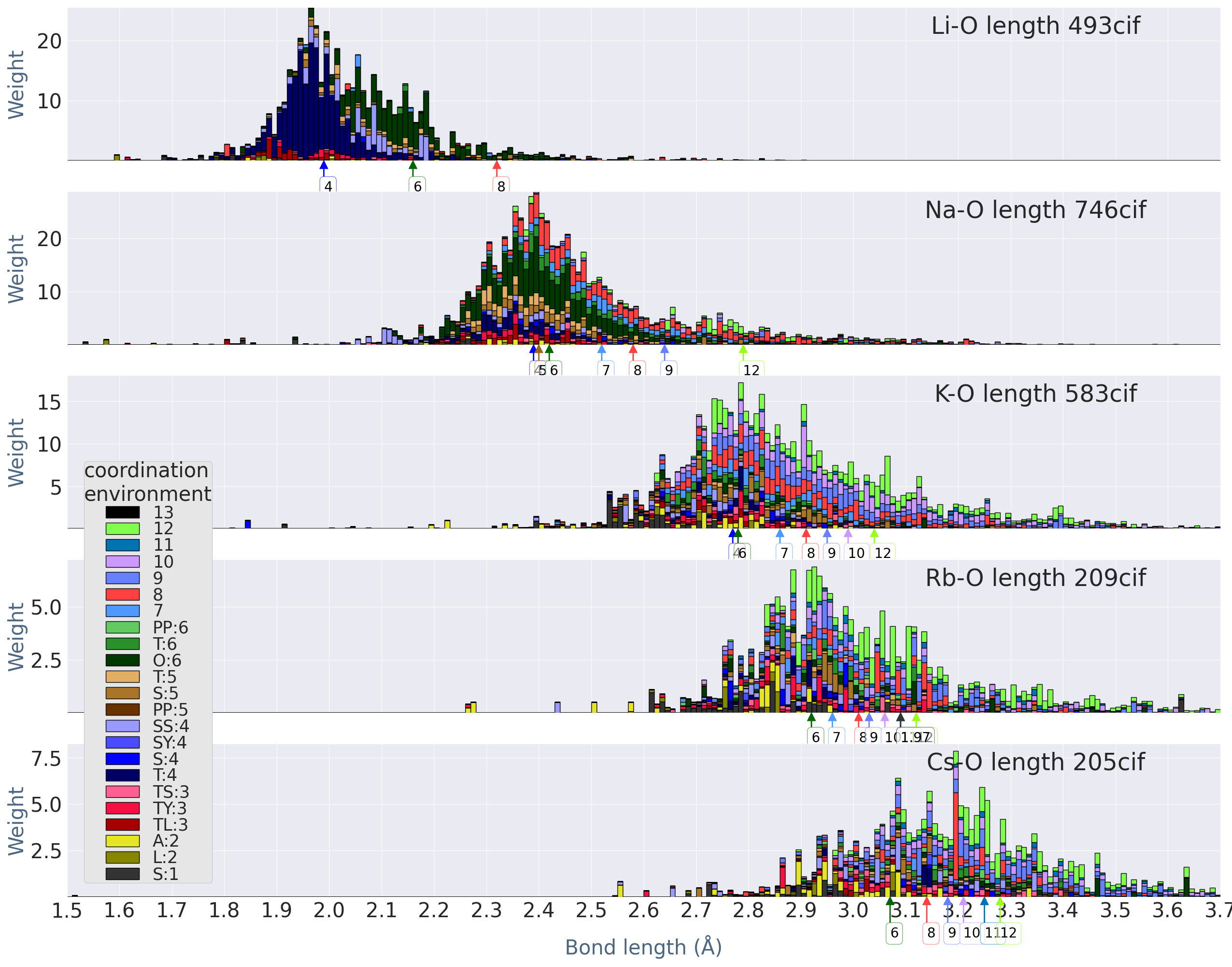
Fig.1 is for the bond-length distributions of alkali and alkali-earth elements. We show histograms $H_{s}(l,C_{\rm env})$, where we accumulate weights in Eq.(1). If we accumulate weight just by CEs neglecting bond-length, the histograms are in agreement with the pie charts in Ref.Waroquiers et al. (2017), except the difference due to the difference of used database. Very outliers shown in our histograms may be or may not be real because of the validation procedures of cifs in COD is still an ongoing problem Vaitkus et al. (2021). For example, we actually found cif files of theoretical models, however, we have not yet removed them because of the difficulty to remove them systematically. Thus our set of cif files should be refined more in future, however, we believe that our overall results will not be altered by such refinement because such refinements affect only to minor outlines.

We show classification to CEs by stacking histograms in order to have over-all view easily. Our histograms show chemical trends of bond-length distribution quite well. We see how the distribution changes for different elements. For CN$>6$, we did not distinguish CE, just showing CN. In our histograms, we resolve CN$<$7 into CEs Waroquiers et al. (2017) as

• •

  S:1 Single neighbor,

• •

  L:2 Linear, A:2 Angular

• •

  TL:3 Trigonal plane, TY:3 Triangular non-coplanar, TS:3 T-shaped,

• •

  T:4 Tetrahedron, S:4 Square plane, SY:4 Square non-coplanar, SS:4 See-saw,

• •

  PP:5 Pentagonal plane, S:5 Square pyramid, T:5 Trigonal bipyramid,

• •

  O:6 Octahedron, T:6 Trigonal prism, PP:6 Pentagonal pyramid,

where numbers show CN.

We see some differences from results from Gagnë and Hawthorne; for example, Na-O for Fig.1 gives a little larger weight for larger bond length than Figure 1 in Ref.Gagné and Hawthorne (2016), although overall features looks to show reasonable agreements. For example, length for CN=6 are distributed around 2.4 Å in agreement with Figure 5 in Ref.Gagné and Hawthorne (2016). The difference can be because of the difference of weight and how we define bonds.

We can observe chemical trend. For Li and Na, we see relatively simple CEs, while K, Rb, Cs show variety of CEs. For Na, we see some amount of weights for both T:5 and S:5. T:4 is dominant for Li and Be, while Li allows some varieties of CEs such as SS:4 and O:6. The length of Be (CN=4) calculated from Shannon’s crystal radii $\sim 1.67$ Å shown by the arrow only slightly larger than the center of the bond-length distribution. The calculated bond length from the radii show similar tendency for other cases.

Figs.2 and 3 are for transition metals. Our results can be compared with that by Gagnë and Hawthorne Gagné and Hawthorne (2020). From the histogram, we can see chemical trends that was not resolved in the pie chart in Ref.Waroquiers et al. (2017). The histogram changes as a function of atomic number, somehow systematically. For example, the peaks of T:4 distribution for V, Cr, and Mn are systematically decreasing. Both Cr and V have peaks of CN=4 and CN=6 at similar lengths, but the widths of distributions is quite narrower for Cr. We see some S:5 weights for V. Histograms for Mn, Fe, Co, and Ni show a systematic changes; two peaks of O:6 at $\sim$1.9 Å and at $\sim$2.2 Å for Mn may correspond to two peaks at $\sim$1.95 Å and at $\sim$2.1 Å for Ni. We see similarity between V and Mo, which belong to the different column of periodic table. Ti and Nb show similarity as well. Sc and Zr, too. From the view of material design, we may like examine possibilities of atomic replacement. For example, the distribution of Ru T:4 and that of Re T:4 is relatively similar, while allows relatively wide range of length for T:4 for Fe. This may suggest one of the condition for the replacement of these atoms each other at T:4 in crystals.

Fig.4 is further classification of V, Fe and Cu of Fig.2 into ion valences, which are determined by the BVS whose parameters are determined in Ref. Gagné and Hawthorne (2015). This is in order to evaluate the idea of BVS. Note that BVS is based on a simple idea to determine the charge transfer via a bond between atoms as a function of length. BVS differentiate Cu⁺ and Cu²⁺ well. Based on the formula of BVS, smaller valence means longer bond length and/or smaller CN. Thus it is reasonable that CN=2 is mainly selected in the case of Cu⁺. We see that shorter bond length are selected for larger valences for Fe and V.

The valence given by BVS is just a parameter to measure how a cation is surrounded. Longer bond length and less number of neighbors gives the same effects to BVS. For example, we can keep the same BVS of a cation when we move four neighbor oxygens away a cation but move another two neighbor oxygens closer simultaneously; BVS claims that such a move do not change the environment of cation in the sense of valence. This sounds reasonable qualitatively, however, we should note the limitation on BVS.

Our histograms have the information of bond length and CEs, without classified by BVS. When we have a new material, its CEs and bond lengths are compared with other materials so as to judge similarity and differences. Our histograms should be a help to perform such comparison.

We have given the histograms of the bond-length distributions of COD, classified by CEs. Our histograms show systematic and non-systematic features of the histograms dependent on species of cations. Our analysis should be a clue to use the bond-weight distribution as the finger print of materials. From the opposite point of view, our challenge is to predict crystal structures as accurate as possible for given composition formula. We believe such ability of prediction can be enhanced with further analysis of crystal structure database along the line of our analysis.

We thank to Prof. Masami Kanzaki for helpful discussions, especially for BVS. This work was partly supported by JSPS KAKENHI Grant Number 17K05499.

References

- Ong et al. (2013) S. P. Ong, W. D. Richards, A. Jain, G. Hautier, M. Kocher, S. Cholia, D. Gunter, V. L. Chevrier, K. A. Persson, and G. Ceder, Computational Materials Science 68, 314 (2013).
- Larsen et al. (2017) A. H. Larsen, J. J. Mortensen, J. Blomqvist, I. E. Castelli, R. Christensen, M. Dułak, J. Friis, M. N. Groves, B. Hammer, C. Hargus, E. D. Hermes, P. C. Jennings, P. B. Jensen, J. Kermode, J. R. Kitchin, E. L. Kolsbjerg, J. Kubal, K. Kaasbjerg, S. Lysgaard, J. B. Maronsson, T. Maxson, T. Olsen, L. Pastewka, A. Peterson, C. Rostgaard, J. Schiøtz, O. Schütt, M. Strange, K. S. Thygesen, T. Vegge, L. Vilhelmsen, M. Walter, Z. Zeng, and K. W. Jacobsen, Journal of Physics: Condensed Matter 29, 273002 (2017).
- Ganose and Jain (2019) A. M. Ganose and A. Jain, MRS Communications 9, 874 (2019).
- Zimmermann and Jain (2020) N. E. R. Zimmermann and A. Jain, RSC Advances 10, 6063 (2020).
- Vaitkus et al. (2021) A. Vaitkus, A. Merkys, and S. Gražulis, Journal of Applied Crystallography 54, 661 (2021).
- Quirós et al. (2018) M. Quirós, S. Gražulis, S. Girdzijauskaitė, A. Merkys, and A. Vaitkus, Journal of Cheminformatics 10, 23 (2018).
- Merkys et al. (2016) A. Merkys, A. Vaitkus, J. Butkus, M. Okulič-Kazarinas, V. Kairys, and S. Gražulis, Journal of Applied Crystallography 49, 292 (2016).
- Gražulis et al. (2012) S. Gražulis, A. Daškevič, A. Merkys, D. Chateigner, L. Lutterotti, M. Quirós, N. R. Serebryanaya, P. Moeck, R. T. Downs, and A. Le Bail, Nucleic Acids Research 40, D420 (2012).
- Gražulis et al. (2009) S. Gražulis, D. Chateigner, R. T. Downs, A. F. T. Yokochi, M. Quirós, L. Lutterotti, E. Manakova, J. Butkus, P. Moeck, and A. Le Bail, Journal of Applied Crystallography 42, 726 (2009).
- Waroquiers et al. (2017) D. Waroquiers, X. Gonze, G.-M. Rignanese, C. Welker-Nieuwoudt, F. Rosowski, M. Göbel, S. Schenk, P. Degelmann, R. André, R. Glaum, and G. Hautier, Chemistry of Materials 29, 8346 (2017).
- Waroquiers et al. (2020) D. Waroquiers, J. George, M. Horton, S. Schenk, K. A. Persson, G.-M. Rignanese, X. Gonze, and G. Hautier, Acta Crystallographica Section B: Structural Science, Crystal Engineering and Materials 76, 683 (2020).
- Gagné and Hawthorne (2016) O. C. Gagné and F. C. Hawthorne, Acta Crystallographica Section B, Structural Science, Crystal Engineering and Materials 72, 602 (2016).
- Gagné and Hawthorne (2020) O. C. Gagné and F. C. Hawthorne, “Bond-length distributions for ions bonded to oxygen: Results for the transition metals and quantification of the factors underlying bond-length variation in inorganic solids,” (2020).
- Gagné and Hawthorne (2015) O. C. Gagné and F. C. Hawthorne, Acta Crystallographica Section B Structural Science, Crystal Engineering and Materials 71, 562 (2015).
- (15) See a supplementary material, https://github.com/Iwamoto0904/Bond_length_distributions.
- Shannon (1976) R. D. Shannon, Acta Crystallographica Section A , 751 (1976).
- (17) A table summarizing Shannon’s radius: at http://abulafia.mt.ic.ac.uk/shannon/radius.php.