Boosted Dynamic Neural Networks
Abstract
Early-exiting dynamic neural networks (EDNN), as one type of dynamic neural networks, has been widely studied recently. A typical EDNN has multiple prediction heads at different layers of the network backbone. During inference, the model will exit at either the last prediction head or an intermediate prediction head where the prediction confidence is higher than a predefined threshold. To optimize the model, these prediction heads together with the network backbone are trained on every batch of training data. This brings a train-test mismatch problem that all the prediction heads are optimized on all types of data in training phase while the deeper heads will only see difficult inputs in testing phase. Treating training and testing inputs differently at the two phases will cause the mismatch between training and testing data distributions. To mitigate this problem, we formulate an EDNN as an additive model inspired by gradient boosting, and propose multiple training techniques to optimize the model effectively. We name our method BoostNet. Our experiments show it achieves the state-of-the-art performance on CIFAR100 and ImageNet datasets in both anytime and budgeted-batch prediction modes. Our code is released at https://github.com/SHI-Labs/Boosted-Dynamic-Networks.
Introduction
Despite the success of the deep learning models on various computer vision tasks, computational resources limitation and inference efficiency must be considered when deploying the models in real-world applications. As a crucial topic in deep learning application, efficient deep learning has been extensively investigated recently, including efficient architecture design (Iandola et al. 2016; Howard et al. 2017; Sandler et al. 2018; Zhang et al. 2018b; Han et al. 2020), network pruning (Han et al. 2015; Han, Mao, and Dally 2016; Li et al. 2016; He, Zhang, and Sun 2017; Luo, Wu, and Lin 2017; He et al. 2019; Lin et al. 2020), and network quantization (Courbariaux et al. 2016; Rastegari et al. 2016; Zhou et al. 2016; Li, Zhang, and Liu 2016; Zhang et al. 2018a; Liu et al. 2018; Wang et al. 2019b; Yu et al. 2019; Liu et al. 2021). Compared with the corresponding large baseline models, these lightweight models usually exhibit significant inference speed-up with small or negligible performance drop.
Dynamic neural networks is another branch of efficient deep learning models. Practically, lightweight models run faster with lower performance, while large models run slower with higher performance. Given a computational resource budget in a specific application scenario, deep learning practitioners often need to find a proper trade-off point between efficiency and performance. However, the budget is often dynamically changed in many scenarios, for example, when the computational resources are largely occupied by other applications or an edge-device’s battery level changes in a day. Therefore, a dynamic neural network (DNN) is desirable that can run at different trade-off points given different resource budgets and performance requirements. Extensive research has been conducted on various dynamic methods including dynamic model architectures, dynamic model parameters, dynamic spatial-wise inference, and more (Teerapittayanon, McDanel, and Kung 2016; Wang et al. 2018; Veit and Belongie 2018; Wu et al. 2018; Yu et al. 2019; Li et al. 2017; Wang et al. 2019a, 2020; Yang et al. 2020; Han et al. 2021). In this paper, we will focus on early-exiting dynamic neural network (EDNN) on image classification tasks, one of most widely explored dynamic architecture methods (Huang et al. 2017; McGill and Perona 2017; Li et al. 2019; Jie et al. 2019; Yang et al. 2020).
EDNN’s adaptive inference property comes from its adjustable layer depth. In inference, when the computational budget is tight or the input example is “easy” to recognize, EDNN exits at a shallow classifier. In the opposite, the model runs through more layers until the last classifier or the classifier that gives a confident prediction. To train such an EDNN model, existing methods usually employ joint optimization over all the classifiers (Huang et al. 2017; Li et al. 2019; Yang et al. 2020). Given a batch of training samples, the model runs through all the layers and classifiers, and the losses are accumulated and summed up. Then the gradients of the total loss are back-propagated to all the layers, and the model parameters are updated accordingly.
One issue in the above training procedure is the train-test mismatch problem, which is also discussed in (Han et al. 2021). In the training stage, all the classifiers in the model are optimized over all the training samples, while in the inference stage, not all the classifiers will see all types of testing data: when the budget is tight or the input is “easy” to process, only shallow layers and classifiers will be executed. In other words, there exists a data distribution gap between the training and testing stages. Although the “easy” examples may also help regularize the deep classifiers in the training stage, the deep classifiers should not be designed to focus too much on these examples in order to avoid the distribution mismatch problem.
To mitigate the train-test mismatch problem, we propose a new type of early-exiting dynamic networks named Boosted Dynamic Neural Networks (BoostNet), inspired by the well-known gradient boosting theory. Assuming the final model is a weighted sum of weak prediction models, gradient boosting algorithms minimize the loss function by iteratively training each weak model with gradient descent in function space. In each training step, the model that points to the negative gradient of the loss function is selected as a new weak model. In this way, each weak model is supplementary to the ensemble of its previous weak models. This property is what we desire in training an EDNN model.
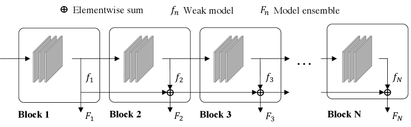
A straightforward manner to incorporate gradient boosting into EDNN training is to directly follow the conventional gradient boosting pipeline to iteratively train the classifiers in the network. However, this does not work well in practice. We speculate there are two main reasons. The first reason is that the deeper classifiers share network layers with the shallower classifiers, so the classifiers are not independent in terms of the network parameters111One may argue to disentangle the classifiers in the EDNN into independent ones. Compared with backbone sharing, training independent classifiers is not efficient in the aspects of model size and computational complexity.. The second reason is that a multi-layer neural network is not a weak prediction model. These two properties do not comply with the assumptions of gradient boosting. Therefore, naïvely training the classifiers in a gradient boosting way will not work. In this paper, we propose BoostNet, which shares the similar spirits of gradient boosting but is organized and trained in a manner adapted to dynamic neural networks. Refer to Fig. 1 for an architecture overview of the proposed BoostNet, where the classifiers are organized as a dynamic-depth neural network with early exits.
To train the model effectively, we propose three training techniques. First, we employ joint optimization over all the classifiers. Training the weak classifiers in the gradient boosting way will lead to a sub-optimal solution for the whole model. On the other hand, training the classifiers sequentially on each training batch is time-costly. Therefore, we train all the classifiers via joint optimization. Second, we propose a prediction reweighting strategy to rescale the ensemble of the previous classifiers before being used an ensemble member of the current classifier. We define a training sample as a valid sample if its training loss is large enough. We experimentally find that the percent of valid training data decreases when the network goes to the deeper classifiers. To avoid the lack of training data for the deep classifiers, we use a temperature to rescale the ensemble of the previous classifiers in order to weaken its prediction. Third, we apply a gradient rescaling technique to the network gradients in order to bound the gradients of parameters at different layer depths. Our ablation study shows this improves the deep classifiers’ performance over the baseline without gradient rescaling.
In summary, the main contributions of this paper are in three folds:
-
•
To our best knowledge, this work is the first attempt to address the train-test mismatch problem in dynamic-depth neural networks with early exits. To this end, we formulate a dynamic neural network as an additive model, and train it in a boosting manner.
-
•
To train the model effectively, we propose several techniques including multi-classifier joint optimization, prediction reweighting, and gradient rescaling techniques.
-
•
The proposed BoostNet achieves the state-of-the-art performance on CIFAR100 and ImageNet datasets in both anytime and budgeted-batch prediction modes.
Related Work
Efficient Neural Networks
To save storage and computational resources, efficient neural networks have been widely studied in the existing works. To this end, a large number of efficient model architectures were designed in the past decade. These architectures include SqueezeNet (Iandola et al. 2016), MobileNets (Howard et al. 2017; Sandler et al. 2018), ShuffleNet (Zhang et al. 2018b), GhostNet (Han et al. 2020), and more. Another branch of efficient methods is network pruning, which removes selected network parameters or even some entire network channels to reduce model redundancy and increase inference speed (Han et al. 2015; Han, Mao, and Dally 2016; Li et al. 2016; He, Zhang, and Sun 2017; Luo, Wu, and Lin 2017; He et al. 2019; Lin et al. 2020). On the other hand, without designing or changing network architectures, the network quantization methods quantize network weights and activations from floating-point values to low-precision integers to allow fast model inference with integer arithmetic (Courbariaux et al. 2016; Rastegari et al. 2016; Zhou et al. 2016; Li, Zhang, and Liu 2016; Zhang et al. 2018a; Liu et al. 2018; Wang et al. 2019b; Yu et al. 2019; Liu et al. 2021).
Dynamic Neural Networks
As a special type of efficient neural networks, dynamic neural networks can adaptively change their inference complexity under different computational budgets, latency requirements, and prediction confidence requirements. Existing dynamic neural networks are designed in different aspects including sample-wise (Teerapittayanon, McDanel, and Kung 2016; Wang et al. 2018; Veit and Belongie 2018; Wu et al. 2018; Yu et al. 2019; Guo et al. 2019), spatial-wise (Li et al. 2017; Wang et al. 2019a, 2020; Yang et al. 2020; Wang et al. 2022a), and temporal-wise dynamism (Shen et al. 2017; Yu, Lee, and Le 2017; Wu et al. 2019; Meng et al. 2020; Wang et al. 2022b), as categorized by (Han et al. 2021). Specially, as one type of sample-wise methods, depth-wise dynamic models with early exits adaptively exit at different layer depths given different inputs (Huang et al. 2017; Li et al. 2019; McGill and Perona 2017; Jie et al. 2019; Yang et al. 2020). In (Huang et al. 2017) and (Li et al. 2019), the authors proposed multi-scale dense networks (MSDNet) to address two issues: a) interference of coarse-level and fine-level neural features, and b) feature scale inconsistency between the shallow and deep classifiers. In (McGill and Perona 2017) and (Jie et al. 2019), different inference exiting policies are proposed for better balance of accuracy and efficiency. In (Yang et al. 2020), resolution adaptive networks (RANet) take multi-scale images as input, based on the intuition that low-resolution features are suitable for high-efficiency inference while high-resolution features are suitable for high-accuracy inference. To train the depth-wise models, these methods jointly minimize the losses of all classifiers on every training batch without considering the dynamic inference property in testing stage. In this paper, we propose a new dynamic architecture BoostNet and several training techniques to mitigate this train-test mismatch problem. For more literature on dynamic neural networks, we refer the readers to (Han et al. 2021) for a comprehensive overview on the relevant papers.
Gradient Boosting
As a pioneering work, AdaBoost was introduced in (Freund and Schapire 1997) to generate a high-accuracy model by combining multiple weak learners/models. The weak learners are optimized sequentially in a way that the subsequent learners pay more attention to the training samples misclassified by the previous classifiers. In (Friedman, Hastie, and Tibshirani 2000) and (Friedman 2001), AdaBoost was generalized to gradient boosting for different loss functions.
Later, gradient boosting methods were combined with neural networks. Following (Freund and Schapire 1997), Schwenk and Bengio applied AdaBoost to neural networks for character classification (Schwenk and Bengio 1998). In recent years, more investigations have been carried out to combine boosting and neural networks. In (Moghimi et al. 2016), BoostCNN was introduced to combine gradient boosting and neural networks for image classification. The model achieved outperforming performance on multiple image classification tasks. In (Cortes et al. 2017), the authors proposed AdaNet to learn neural network structure and parameters at the same time. The network was optimized over a generalization bound which is composed of a task loss and a regularization term. In (Huang et al. 2018), ResNet (He et al. 2016) was built sequentially in a gradient boosting way. The resulted BoostResNet required less computational and memory resources, and had exponentially decaying training errors as the layer depth increases. More recently, GrowNet was proposed to train neural networks with gradient boosting (Badirli et al. 2020), where shallow neural networks were regarded as “weak classifiers”. In addition, after a layer is trained, a corrective finetuning step is applied to all the previous layers to improve the model performance. Different from these existing works, our training framework is designed for dynamic network structure and adaptive inference ability. To this end, we propose several optimization techniques to train the model effectively.
Boosted Dynamic Neural Networks
Overview
An EDNN model usually consists of multiple stacked sub-models. In inference time, given an input image, we run the model until the last layer of the first classifier to get a coarse prediction. If the prediction result is confident above a predefined threshold, the inference can be terminated at just the first classifier. Otherwise, the second classifier will be executed on the features from the first classifier. It is expected to give a more confident prediction, correcting the mistake made by the first classifier. If not, we repeat the above process until either some classifier gives a confident enough prediction or the last classifier is reached.
To train the model, existing EDNN methods train all the classifiers jointly without considering the adaptive inference property described above (Huang et al. 2017; Li et al. 2019; Yang et al. 2020). Considering an -classifier EDNN model, the overall task loss will be
| (1) |
where and are an input example and its true categorical label, and are -th classifier’s prediction and its contribution to the overall loss. This makes all the classifiers treat every training sample the same way. However, in inference time, the model will exit at early classifiers on easy inputs, so the deep classifiers will only be executed on difficult ones. This train-test mismatch problem will cause a data distribution gap between model training and testing stages, rendering a trained model sub-optimal.
Rethinking the inference process above, we find the intrinsic property of EDNN model is that a deeper classifier is supplementary to its previous classifiers by correcting their mistakes. This property shares a similar spirit with gradient boosting methods.
First we give a brief overview of the gradient boosting theory. Given an input and its output , gradient boosting is to find some function to approximate the output . is in form of a sum of multiple base classifiers as
| (2) |
where is a constant. Gradient boosting optimizes each weak classifier sequentially:
| (3) | ||||
where is a scalar and is some function class. Directly optimizing this problem to find the optimal is difficult given an arbitrary loss function . Gradient boosting methods make a first-order approximation to Eq. 3. As a result, we have
| (4) |
where is the learning rate.
Inspired by gradient boosting, we organize the classifiers of EDNN in a similar structure. The final output of the -th block is a linear combination of the outputs of -th block and all its previous blocks. Fig. 1 shows the proposed network structure. We name this architecture Boosted Dynamic Neural Networks (BoostNet).
Different from the first-order approximation in gradient boosting, we directly optimize the neural network w.r.t. parameters with mini-batch gradient descent for multiple steps:
| (5) | ||||
where ’s gradient is disabled even if it shares a subset of parameters with as shown in Fig. 1. In the ablation studies, we will compare this setting with the case of differentiable , and find disabling ’s gradient works better.
Mini-batch Joint Optimization
Following traditional gradient boosting methods, one straight-forward optimization procedure is to train the classifiers sequentially, That is, train classifier until convergence, fix its classification head, and train . However, this makes all classifiers shallower than deteriorate when training because all the classifiers share the same network backbone. On the other hand, fixing the shared parameters and only training ’s non-shared parameters will hurt its representation capacity.
Instead, we employ a mini-batch joint optimization scheme. Given a mini-batch of training data, we forward the entire BoostNet to get prediction outputs. Then we sum up the training losses over the outputs and take one back-propagation step. The overall loss is
| (6) |
We experimentally find works well.
Model with parameters for network blocks.
Classifiers’ intermediate outputs .
Classifiers’ final outputs .
Prediction temperatures .
Training dataset .
Model
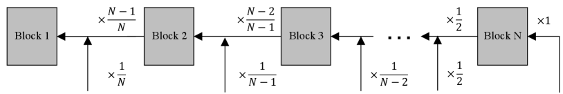
Gradient Rescaling
Similar to (Li et al. 2019), we use a gradient rescaling operation to rescale the gradients from different network branches. As shown in Fig. 2, we multiply a scalar in each branch to rescale the gradients that pass through it. With this operation, the gradient of the overall loss w.r.t. block is
| (7) |
which is bounded even if is a large number, given the weak assumption that is bounded, which is usually true. The effectiveness of gradient rescaling will be demonstrated in the ablation studies.
| MSDNet | RANet | |||||||||||||||||
|---|---|---|---|---|---|---|---|---|---|---|---|---|---|---|---|---|---|---|
| Classifier index | 1 | 2 | 3 | 4 | 5 | 6 | 7 | 8 | 9 | 10 | 1 | 2 | 3 | 4 | 5 | 6 | 7 | 8 |
| Mul-Add () | 15.14 | 25.51 | 37.79 | 52.06 | 62.18 | 74.07 | 87.73 | 100.0 | 110.1 | 121.7 | 15.83 | 31.31 | 44.69 | 50.40 | 60.71 | 63.72 | 90.26 | 95.00 |
| Baseline | 64.60 | 67.94 | 69.36 | 71.53 | 72.76 | 74.03 | 74.65 | 75.37 | 75.53 | 75.98 | 66.71 | 69.11 | 71.22 | 71.99 | 72.86 | 72.93 | 73.88 | 74.69 |
| Ours | 65.32 | 70.01 | 72.34 | 74.15 | 75.24 | 75.85 | 75.94 | 76.51 | 76.53 | 76.30 | 67.53 | 70.83 | 73.17 | 73.39 | 74.20 | 74.05 | 74.75 | 75.08 |
| MSDNet | RANet | ||||||||||||
|---|---|---|---|---|---|---|---|---|---|---|---|---|---|
| Classifier index | 1 | 2 | 3 | 4 | 5 | 6 | 7 | 8 | 1 | 2 | 3 | 4 | 5 |
| Mul-Add () | 435.0 | 888.7 | 1153 | 1352 | 2280 | 2588 | 3236 | 3333 | 615.7 | 1436 | 2283 | 2967 | 3254 |
| Baseline | 63.29 | 67.59 | 69.90 | 70.84 | 74.25 | 74.73 | 74.29 | 74.46 | 63.69 | 71.12 | 73.60 | 74.46 | 75.24 |
| Ours | 64.19 | 68.33 | 71.07 | 71.53 | 74.54 | 74.90 | 75.09 | 74.66 | 64.78 | 71.63 | 74.48 | 75.35 | 76.05 |
Prediction Reweighting with Temperature
When training in the above procedure, we observed a problem that the deeper classifiers do not show much performance improvement over the shallow classifiers, although the model size increases by a large margin.
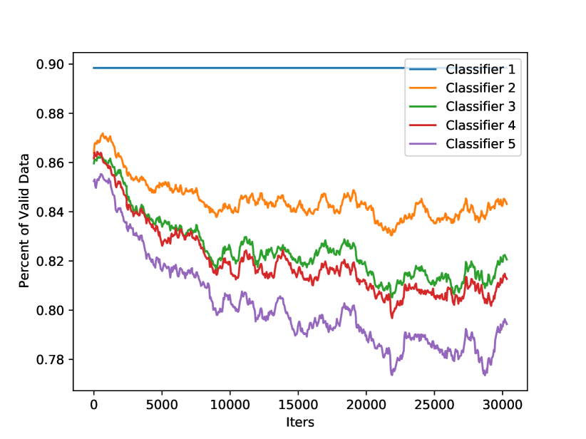
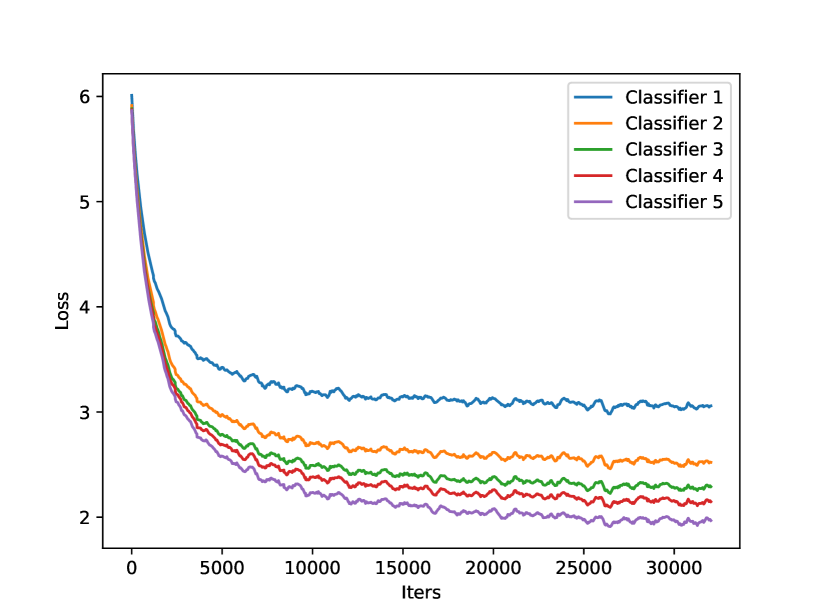
We found this is caused by insufficient training data for deeper classifiers. In Fig. 3(a), we show the number of valid training samples for each classifier. A training sample is valid if its training loss is larger than a certain threshold . Here, we set to be the 10-th percentile of all the training losses of the first classifier in each batch of training data, i.e., we assume the first classifier always has valid training samples. From the figure, we find the shallower classifiers have more valid training data while the deeper classifiers have relatively less. In Fig. 3(b), we show the batch-wise average training losses of different classifiers. Consistent with Fig. 3(a), the deeper classifiers have smaller training losses. From another perspective, this can be explained by the fact that the deeper classifiers have a larger model size and thus more representation power, but this also indicates that the deeper classifiers need more challenging training samples instead of learning the “easy” residuals of the shallower classifiers.
To address this problem, we multiply the output of -th classifier by a temperature before serving as an ensemble member of as
| (8) |
where and are pre-softmax prediction logits. We set all the temperatures to in our experiments unless specified in the ablation studies. We name this technique prediction reweighting. With this, the ensemble output of the shallow classifiers is equivalent to being weakened before being used in the ensemble output .
With the proposed training techniques, the overall training pipeline is summarized in Algorithm 1.
Experiments
Settings
To evaluate the proposed method, we apply it to two different network backbones, MSDNet (Huang et al. 2017) and RANet (Yang et al. 2020), both of which are dynamic models designed for adaptive inference. It is noted that our method is model-agnostic, and can also be applied to other network backbones. We do experiments on two datasets, CIFAR100 (Krizhevsky 2009) and ImageNet (Deng et al. 2009) , in two prediction modes, anytime prediction mode and budgeted-batch prediction mode following (Huang et al. 2017; Yang et al. 2020). In anytime prediction mode, the model runs at a fixed computational budget for all inputs. In budgeted-batch prediction mode, the model runs at an average budget, which means it can have different inference costs for different inputs as long as the overall average cost is below a threshold. To calculate the confidence threshold determining whether the model exits or not, we randomly reserve 5000 samples in CIFAR100 and 50000 samples in ImageNet as a validation set. We utilize a similar model combination strategy to (Huang et al. 2017; Yang et al. 2020). That is, we train a single dynamic model for anytime mode on both datasets. For budgeted-batch mode, we train multiple models with different model sizes for each dataset.
For MSDNet (Huang et al. 2017), we use the same model configurations as the original model except the CIFAR100-Batch models. In (Huang et al. 2017), the classifiers are located at depths , where is , , or for the three different models. One problem with this setting is that the three models have the same representation capacity for the shallow classifiers, which causes redundant overlap of computational complexity. Instead, we set the locations as , where is , , or for the three models. Thus, each model has classifiers at different depths. For RANet (Yang et al. 2020), we follow the same settings as the original paper. For prediction reweighting, we set all temperatures .
For CIFAR100, the models are trained for epochs with SGD optimizer with momentum and initial learning rate . The learning rate is decayed at epochs and . We use single GPU with training batch size . For ImageNet, the models are trained for epochs with SGD optimizer with momentum and initial learning rate . The learning rate is decayed at epochs and . We use GPUs with training batch size on each GPU. Our training framework is implemented in PyTorch (Paszke et al. 2019).
Anytime Prediction Mode
In this section, we compare our method with MSDNet and RANet in the anytime prediction mode. We also apply gradient rescaling to the baseline models. The results on CIFAR100 and ImageNet are plotted in Tab. 1 and 2. On both datasets, our model achieves better results under the same computational budget measured in Multi-Add. The improvement is even more significant under the low computational budgets on CIFAR100.
Budgeted-batch Prediction Mode
In budgeted-batch prediction mode, we set a computational complexity upper bound such that the average computational cost of the input images is below this value. We assume a proportion of samples exit at every classifier. Therefore, the average computational cost will be
| (9) |
where is the number of classifiers and is the computational complexity of layers between block and . Given a budget threshold, we can utilize the Newton–Raphson method to find a satisfying the equation. Finally, we run the model on the hold-out evaluation set to determine the confidence threshold for each classifier given exiting probability . We define the confidence of a classifier as its maximum softmax probability over all the categories.
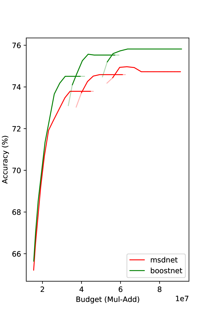
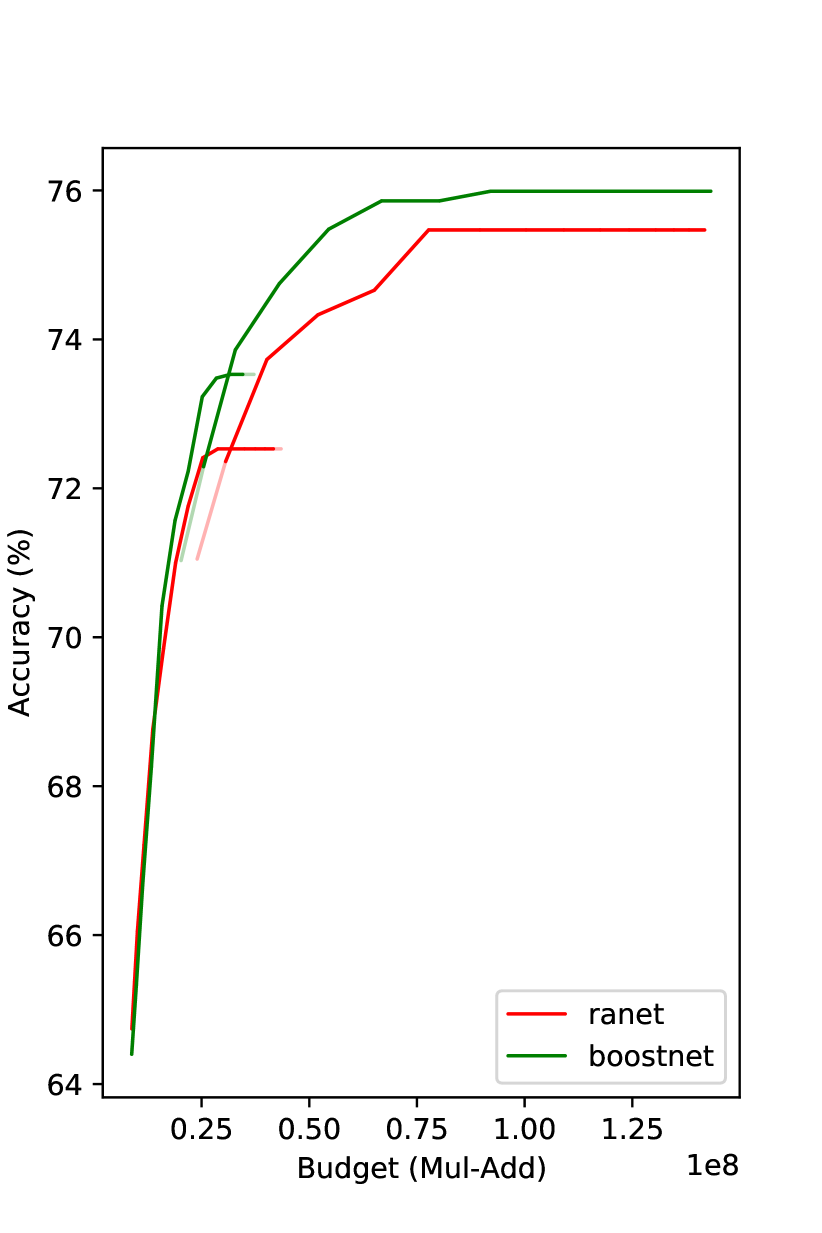
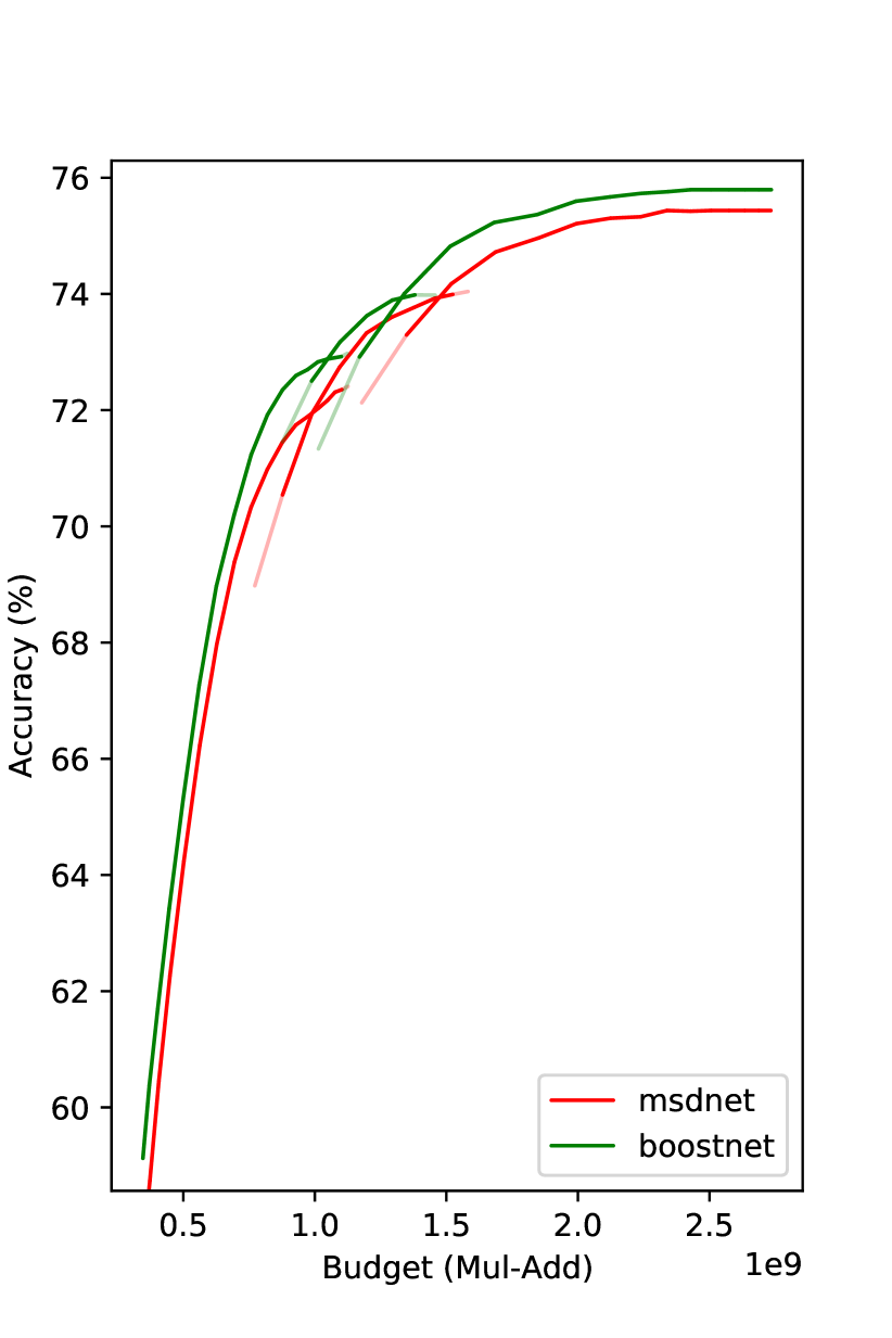
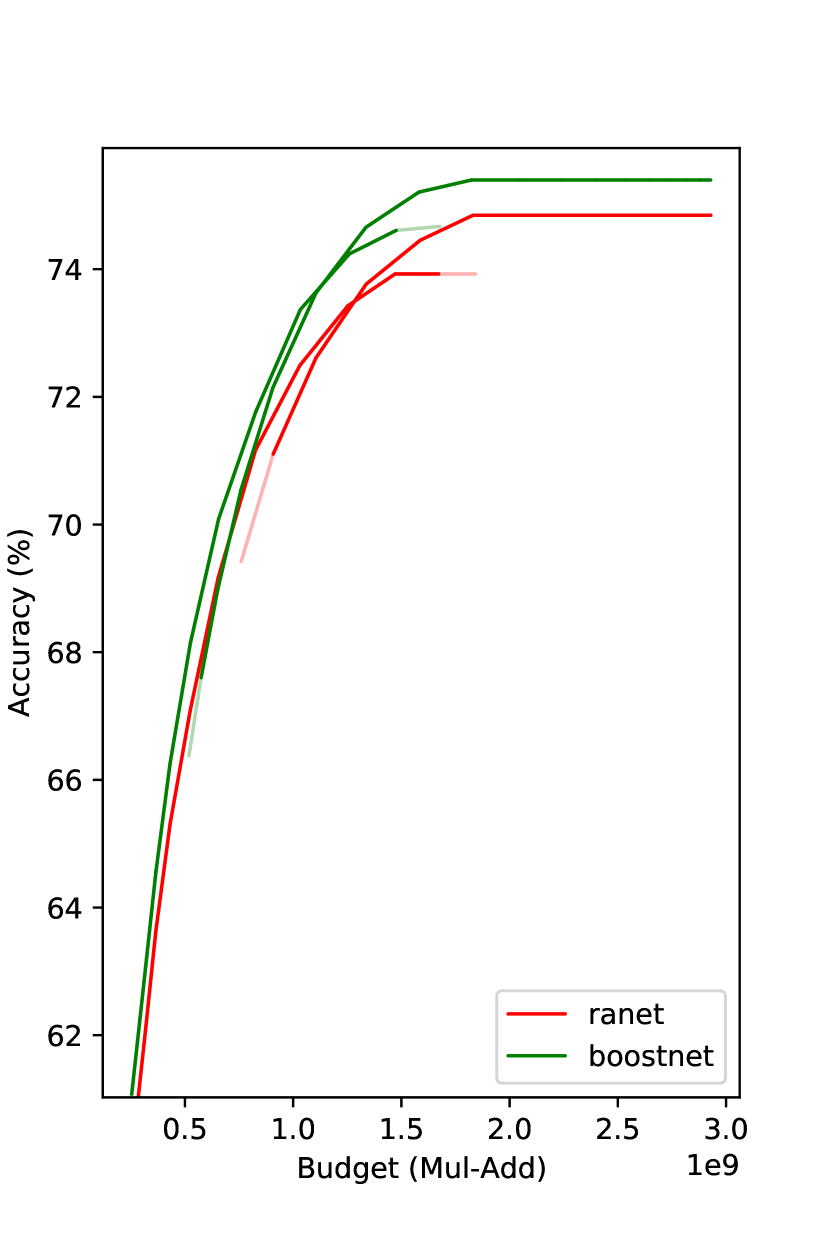
We compare our method with MSDNet and RANet in Fig. 4.222Due to various reasons, e.g., different validation sets, RANet’s CIFAR100 result here may be a bit different from that in the paper. Under the same budget, our method gets superior results. On CIFAR100, the improvement over MSDNet is even more than . We observe that the improvement decreases as the budget increases. We speculate the reason is when the model goes deeper, the effective amount of training data decreases. The proposed prediction reweighting technique mitigates this problem, but it is not entirely eliminated.
Note that the curve tails are flat in Fig. 4(a) and Fig. 4(b), i.e., a deeper classifier does not improve the performance over a shallower one. One possible reason of such a phenomenon of diminishing returns is overfitting. To avoid performance drop when computational budget increases, we do not increase confidence threshold if this change does not bring performance improvement. This process is conducted on the hold-out evaluation dataset. A similar strategy is also employed in (Yang et al. 2020).
Inference Visualization
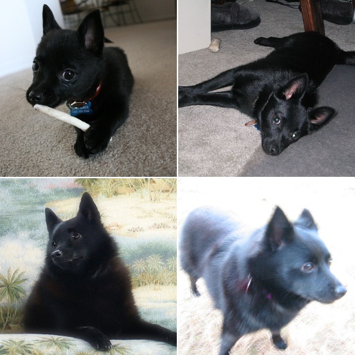
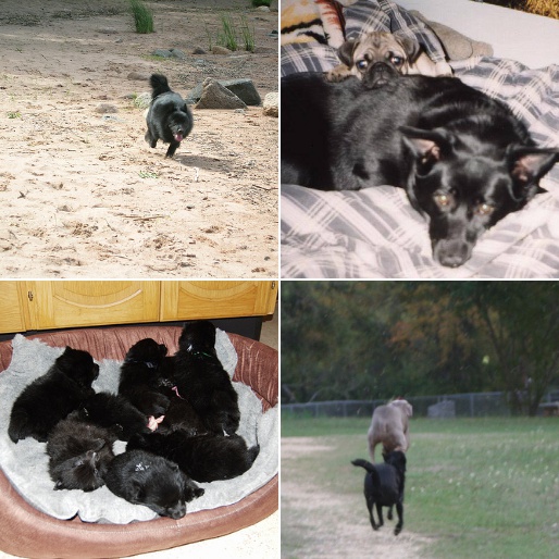
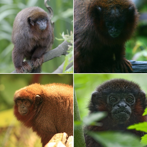
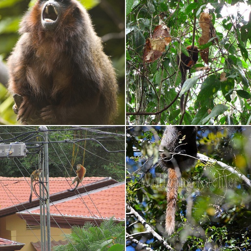
We show visual examples that exit at various depths of the dynamic model. Fig. 5(a) and 5(b) are schipperke images that exit at classifier and respectively. Fig. 5(c) and 5(d) are titi examples exiting at classifier and respectively. We find that image instances exiting at classifier are usually “easier” than those exiting at classifier . Actually, this phenomenon can be observed in all the categories in ImageNet. Generally, images with occlusion, small object size, unusual view angle, and complex background are difficult to recognize and require a deeper classifier.
Ablation Studies
In this section, we do ablation experiments using MSDNet backbone to understand the training techniques.
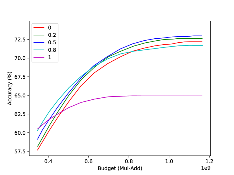
Prediction reweighting. In the previous section, we introduced prediction reweighting to make sure more valid training data for deeper classifiers. In this part, we study how prediction reweighting temperature affects the performance. The results are plotted in Fig. 6(a). We find that the deeper classifiers cannot learn well without enough supervision when is , although the shallower classifiers achieve better performance than the other values. On the other hand, when is , it basically becomes an MSDNet, which also performs inferior to the case of . As a trade-off, we set in all our experiments.
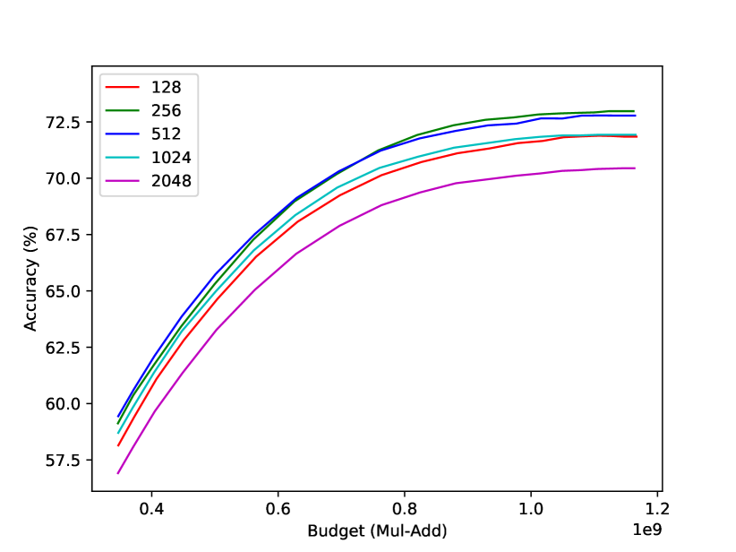
Batch size. As introduced earlier, we formulated the early-exiting dynamic-depth neural network as an additive model in a way that the prediction of a deep classifier depends on all its preceding classifiers . At training step , is computed using before the new are computed. Intuitively thinking, if these shallower classifiers fluctuate too much during training, the deeper classifier cannot be well learned. Therefore, a relatively large batch size is desired for better training stability. Meanwhile, it cannot be too large to hurt the model’s generalization ability (Keskar et al. 2016). Therefore, batch size plays an important role in dynamic network training. In Fig. 6(b), we show how batch size affects the classification performance. Both too large batch sizes and too small batch sizes get worse performance. Therefore, we set the batch size to be for CIFAR100 models and for ImageNet models as a trade-off between stability and generalization.
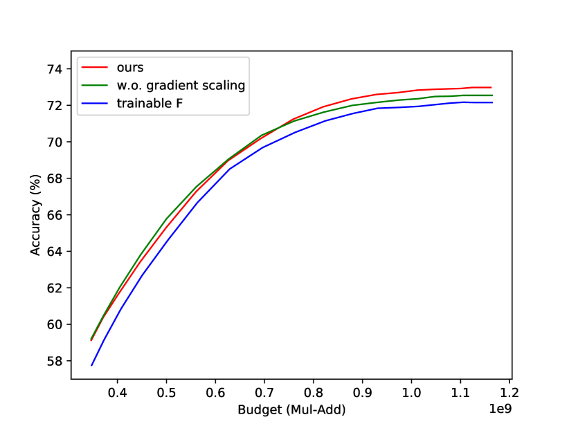
Gradient rescaling. In Fig. 6(c), we compare the model with gradient rescaling (red curve) and that without gradient rescaling (green curve). When the budget is over , the model with gradient rescaling gets better performance than that without it. This shows gradient rescaling can help improve the performance of the deeper classifiers.
Trainable . As shown in Algorithm 1, we do not back-propagate gradients of along branch. We do this to avoid entangling deeper losses in shallower classifiers. For comparison purpose, we train a model without cutting out the gradients of w.r.t. . The results are shown as the blue curve in Fig. 6(c). Entangling deeper losses in shallower classifiers hurts classification performance.
Discussion
To analyze the training process of the deep classifiers in the proposed BoostNet, we introduced the concept of effective training data in dynamic network training. It measures the proportion of training samples that have large enough losses for effectively training a classifier. To make a trade-off between solving train-test mismatch problem and increasing the proportion of effective training data, we introduced a prediction reweighting temperature to weaken the prediction of the early classifiers. One future research topic is to design a better metric to evaluate the amount of effective training data, and a better prediction reweighting algorithm. For instance, use a dynamic temperature that adaptively adjusts the effective training data amount for different classifiers on each training batch.
Dynamic-depth neural networks can be regarded as a combination of multiple sub-models, each of which concentrates on a subset of training data. Existing methods train all the sub-models on all the training data. Our method trains the first sub-model on all the data, and deeper sub-models on the hard samples. Another possibility is to train different sub-models on different subsets, avoiding training the shallower classifiers on the hard samples and the deeper classifiers on the easy samples. In this case, a model selection module is needed to determine which sub-model should be used for an input. A similar idea is explored in (Zhang, Chen, and Zhong 2021), where an expert selection module is proposed to do expert (sub-model) selection. However, their model is not designed for adaptive inference, and the low-level feature extraction module is not shared among the experts for better inference efficiency.
Our method has some limitations. First, BoostNet is mainly designed for image classification tasks. For other tasks like object detection and semantic segmentation, it would be difficult to determine if an input is easy or difficult at the image level since we make pixel-level or region-level predictions. Applying our method to other vision tasks is still under exploration. Second, there exists an efficiency gap between theoretical analysis and real-world application on different hardware. Traditional neural networks can be executed in parallel via batch inference, but the adaptive inference models like the proposed BoostNet need a special design to allow better batch inference since the model has different inference paths on different inputs.
Conclusion
In this paper, we introduced a Boosted Dynamic Neural Network architecture. Different from existing dynamic-depth neural networks, we formulate our dynamic network as an additive model similar to gradient boosting in order to solve the train-test mismatch problem. To optimize the model effectively, we jointly update all the classifiers at the same time, which avoids the classifiers falling into sub-optimal solutions. In addition, we propose prediction reweighting with temperature to increase the amount of effective training data for deep classifiers. To bound the gradients from all classifiers, we leverage gradient rescaling to rescale the gradients from each branch. Our method achieves superior performance on CIFAR100 and ImageNet datasets in both anytime and budgeted-batch prediction modes.
References
- Badirli et al. (2020) Badirli, S.; Liu, X.; Xing, Z.; Bhowmik, A.; Doan, K.; and Keerthi, S. S. 2020. Gradient boosting neural networks: Grownet. arXiv preprint arXiv:2002.07971.
- Cortes et al. (2017) Cortes, C.; Gonzalvo, X.; Kuznetsov, V.; Mohri, M.; and Yang, S. 2017. Adanet: Adaptive structural learning of artificial neural networks. In International conference on machine learning, 874–883. PMLR.
- Courbariaux et al. (2016) Courbariaux, M.; Hubara, I.; Soudry, D.; El-Yaniv, R.; and Bengio, Y. 2016. Binarized neural networks: Training deep neural networks with weights and activations constrained to+ 1 or-1. arXiv preprint arXiv:1602.02830.
- Deng et al. (2009) Deng, J.; Dong, W.; Socher, R.; Li, L.-J.; Li, K.; and Fei-Fei, L. 2009. Imagenet: A large-scale hierarchical image database. In 2009 IEEE conference on computer vision and pattern recognition, 248–255. Ieee.
- Freund and Schapire (1997) Freund, Y.; and Schapire, R. E. 1997. A decision-theoretic generalization of on-line learning and an application to boosting. Journal of computer and system sciences, 55(1): 119–139.
- Friedman, Hastie, and Tibshirani (2000) Friedman, J.; Hastie, T.; and Tibshirani, R. 2000. Additive logistic regression: a statistical view of boosting (with discussion and a rejoinder by the authors). The annals of statistics, 28(2): 337–407.
- Friedman (2001) Friedman, J. H. 2001. Greedy function approximation: a gradient boosting machine. Annals of statistics, 1189–1232.
- Guo et al. (2019) Guo, Y.; Shi, H.; Kumar, A.; Grauman, K.; Rosing, T.; and Feris, R. 2019. Spottune: transfer learning through adaptive fine-tuning. In Proceedings of the IEEE/CVF conference on computer vision and pattern recognition, 4805–4814.
- Han et al. (2020) Han, K.; Wang, Y.; Tian, Q.; Guo, J.; Xu, C.; and Xu, C. 2020. Ghostnet: More features from cheap operations. In Proceedings of the IEEE/CVF Conference on Computer Vision and Pattern Recognition, 1580–1589.
- Han, Mao, and Dally (2016) Han, S.; Mao, H.; and Dally, W. J. 2016. Deep Compression: Compressing Deep Neural Networks with Pruning, Trained Quantization and Huffman Coding. International Conference on Learning Representations (ICLR).
- Han et al. (2015) Han, S.; Pool, J.; Tran, J.; and Dally, W. 2015. Learning both Weights and Connections for Efficient Neural Network. In Cortes, C.; Lawrence, N.; Lee, D.; Sugiyama, M.; and Garnett, R., eds., Advances in Neural Information Processing Systems, volume 28. Curran Associates, Inc.
- Han et al. (2021) Han, Y.; Huang, G.; Song, S.; Yang, L.; Wang, H.; and Wang, Y. 2021. Dynamic neural networks: A survey. arXiv preprint arXiv:2102.04906.
- He et al. (2016) He, K.; Zhang, X.; Ren, S.; and Sun, J. 2016. Deep residual learning for image recognition. In Proceedings of the IEEE conference on computer vision and pattern recognition, 770–778.
- He et al. (2019) He, Y.; Liu, P.; Wang, Z.; Hu, Z.; and Yang, Y. 2019. Filter pruning via geometric median for deep convolutional neural networks acceleration. In Proceedings of the IEEE/CVF Conference on Computer Vision and Pattern Recognition, 4340–4349.
- He, Zhang, and Sun (2017) He, Y.; Zhang, X.; and Sun, J. 2017. Channel pruning for accelerating very deep neural networks. In Proceedings of the IEEE international conference on computer vision, 1389–1397.
- Howard et al. (2017) Howard, A. G.; Zhu, M.; Chen, B.; Kalenichenko, D.; Wang, W.; Weyand, T.; Andreetto, M.; and Adam, H. 2017. Mobilenets: Efficient convolutional neural networks for mobile vision applications. arXiv preprint arXiv:1704.04861.
- Huang et al. (2018) Huang, F.; Ash, J.; Langford, J.; and Schapire, R. 2018. Learning deep resnet blocks sequentially using boosting theory. In International Conference on Machine Learning, 2058–2067. PMLR.
- Huang et al. (2017) Huang, G.; Chen, D.; Li, T.; Wu, F.; van der Maaten, L.; and Weinberger, K. Q. 2017. Multi-scale dense networks for resource efficient image classification. arXiv preprint arXiv:1703.09844.
- Iandola et al. (2016) Iandola, F. N.; Han, S.; Moskewicz, M. W.; Ashraf, K.; Dally, W. J.; and Keutzer, K. 2016. SqueezeNet: AlexNet-level accuracy with 50x fewer parameters and¡ 0.5 MB model size. arXiv preprint arXiv:1602.07360.
- Jie et al. (2019) Jie, Z.; Sun, P.; Li, X.; Feng, J.; and Liu, W. 2019. Anytime Recognition with Routing Convolutional Networks. IEEE transactions on pattern analysis and machine intelligence.
- Keskar et al. (2016) Keskar, N. S.; Mudigere, D.; Nocedal, J.; Smelyanskiy, M.; and Tang, P. T. P. 2016. On large-batch training for deep learning: Generalization gap and sharp minima. arXiv preprint arXiv:1609.04836.
- Krizhevsky (2009) Krizhevsky, A. 2009. Learning multiple layers of features from tiny images. Technical report.
- Li, Zhang, and Liu (2016) Li, F.; Zhang, B.; and Liu, B. 2016. Ternary weight networks. arXiv preprint arXiv:1605.04711.
- Li et al. (2016) Li, H.; Kadav, A.; Durdanovic, I.; Samet, H.; and Graf, H. P. 2016. Pruning filters for efficient convnets. arXiv preprint arXiv:1608.08710.
- Li et al. (2019) Li, H.; Zhang, H.; Qi, X.; Yang, R.; and Huang, G. 2019. Improved techniques for training adaptive deep networks. In Proceedings of the IEEE/CVF International Conference on Computer Vision, 1891–1900.
- Li et al. (2017) Li, Z.; Yang, Y.; Liu, X.; Zhou, F.; Wen, S.; and Xu, W. 2017. Dynamic computational time for visual attention. In Proceedings of the IEEE International Conference on Computer Vision Workshops, 1199–1209.
- Lin et al. (2020) Lin, M.; Ji, R.; Wang, Y.; Zhang, Y.; Zhang, B.; Tian, Y.; and Shao, L. 2020. Hrank: Filter pruning using high-rank feature map. In Proceedings of the IEEE/CVF Conference on Computer Vision and Pattern Recognition, 1529–1538.
- Liu et al. (2021) Liu, Z.; Wang, Y.; Han, K.; Zhang, W.; Ma, S.; and Gao, W. 2021. Post-training quantization for vision transformer. Advances in Neural Information Processing Systems, 34.
- Liu et al. (2018) Liu, Z.; Wu, B.; Luo, W.; Yang, X.; Liu, W.; and Cheng, K.-T. 2018. Bi-real net: Enhancing the performance of 1-bit cnns with improved representational capability and advanced training algorithm. In Proceedings of the European conference on computer vision (ECCV), 722–737.
- Luo, Wu, and Lin (2017) Luo, J.-H.; Wu, J.; and Lin, W. 2017. Thinet: A filter level pruning method for deep neural network compression. In Proceedings of the IEEE international conference on computer vision, 5058–5066.
- McGill and Perona (2017) McGill, M.; and Perona, P. 2017. Deciding how to decide: Dynamic routing in artificial neural networks. In International Conference on Machine Learning, 2363–2372. PMLR.
- Meng et al. (2020) Meng, Y.; Lin, C.-C.; Panda, R.; Sattigeri, P.; Karlinsky, L.; Oliva, A.; Saenko, K.; and Feris, R. 2020. Ar-net: Adaptive frame resolution for efficient action recognition. In European Conference on Computer Vision, 86–104. Springer.
- Moghimi et al. (2016) Moghimi, M.; Belongie, S. J.; Saberian, M. J.; Yang, J.; Vasconcelos, N.; and Li, L.-J. 2016. Boosted Convolutional Neural Networks. In BMVC, volume 5, 6.
- Paszke et al. (2019) Paszke, A.; Gross, S.; Massa, F.; Lerer, A.; Bradbury, J.; Chanan, G.; Killeen, T.; Lin, Z.; Gimelshein, N.; Antiga, L.; Desmaison, A.; Kopf, A.; Yang, E.; DeVito, Z.; Raison, M.; Tejani, A.; Chilamkurthy, S.; Steiner, B.; Fang, L.; Bai, J.; and Chintala, S. 2019. PyTorch: An Imperative Style, High-Performance Deep Learning Library. In Wallach, H.; Larochelle, H.; Beygelzimer, A.; d'Alché-Buc, F.; Fox, E.; and Garnett, R., eds., Advances in Neural Information Processing Systems 32, 8024–8035. Curran Associates, Inc.
- Rastegari et al. (2016) Rastegari, M.; Ordonez, V.; Redmon, J.; and Farhadi, A. 2016. Xnor-net: Imagenet classification using binary convolutional neural networks. In European conference on computer vision, 525–542. Springer.
- Sandler et al. (2018) Sandler, M.; Howard, A.; Zhu, M.; Zhmoginov, A.; and Chen, L.-C. 2018. Mobilenetv2: Inverted residuals and linear bottlenecks. In Proceedings of the IEEE conference on computer vision and pattern recognition, 4510–4520.
- Schwenk and Bengio (1998) Schwenk, H.; and Bengio, Y. 1998. Training methods for adaptive boosting of neural networks for character recognition. Advances in neural information processing systems, 10: 647–653.
- Shen et al. (2017) Shen, Y.; Huang, P.-S.; Gao, J.; and Chen, W. 2017. Reasonet: Learning to stop reading in machine comprehension. In Proceedings of the 23rd ACM SIGKDD International Conference on Knowledge Discovery and Data Mining, 1047–1055.
- Teerapittayanon, McDanel, and Kung (2016) Teerapittayanon, S.; McDanel, B.; and Kung, H.-T. 2016. Branchynet: Fast inference via early exiting from deep neural networks. In 2016 23rd International Conference on Pattern Recognition (ICPR), 2464–2469. IEEE.
- Veit and Belongie (2018) Veit, A.; and Belongie, S. 2018. Convolutional networks with adaptive inference graphs. In Proceedings of the European Conference on Computer Vision (ECCV), 3–18.
- Wang et al. (2019a) Wang, H.; Kembhavi, A.; Farhadi, A.; Yuille, A. L.; and Rastegari, M. 2019a. Elastic: Improving cnns with dynamic scaling policies. In Proceedings of the IEEE/CVF Conference on Computer Vision and Pattern Recognition, 2258–2267.
- Wang et al. (2019b) Wang, K.; Liu, Z.; Lin, Y.; Lin, J.; and Han, S. 2019b. Haq: Hardware-aware automated quantization with mixed precision. In Proceedings of the IEEE/CVF Conference on Computer Vision and Pattern Recognition, 8612–8620.
- Wang et al. (2018) Wang, X.; Yu, F.; Dou, Z.-Y.; Darrell, T.; and Gonzalez, J. E. 2018. Skipnet: Learning dynamic routing in convolutional networks. In Proceedings of the European Conference on Computer Vision (ECCV), 409–424.
- Wang et al. (2020) Wang, Y.; Lv, K.; Huang, R.; Song, S.; Yang, L.; and Huang, G. 2020. Glance and focus: a dynamic approach to reducing spatial redundancy in image classification. arXiv preprint arXiv:2010.05300.
- Wang et al. (2022a) Wang, Y.; Yue, Y.; Lin, Y.; Jiang, H.; Lai, Z.; Kulikov, V.; Orlov, N.; Shi, H.; and Huang, G. 2022a. Adafocus v2: End-to-end training of spatial dynamic networks for video recognition. In 2022 IEEE/CVF Conference on Computer Vision and Pattern Recognition (CVPR), 20030–20040. IEEE.
- Wang et al. (2022b) Wang, Y.; Yue, Y.; Xu, X.; Hassani, A.; Kulikov, V.; Orlov, N.; Song, S.; Shi, H.; and Huang, G. 2022b. AdaFocusV3: On Unified Spatial-Temporal Dynamic Video Recognition. In European Conference on Computer Vision, 226–243. Springer.
- Wu et al. (2018) Wu, Z.; Nagarajan, T.; Kumar, A.; Rennie, S.; Davis, L. S.; Grauman, K.; and Feris, R. 2018. Blockdrop: Dynamic inference paths in residual networks. In Proceedings of the IEEE Conference on Computer Vision and Pattern Recognition, 8817–8826.
- Wu et al. (2019) Wu, Z.; Xiong, C.; Ma, C.-Y.; Socher, R.; and Davis, L. S. 2019. Adaframe: Adaptive frame selection for fast video recognition. In Proceedings of the IEEE/CVF Conference on Computer Vision and Pattern Recognition, 1278–1287.
- Yang et al. (2020) Yang, L.; Han, Y.; Chen, X.; Song, S.; Dai, J.; and Huang, G. 2020. Resolution adaptive networks for efficient inference. In Proceedings of the IEEE/CVF Conference on Computer Vision and Pattern Recognition, 2369–2378.
- Yu, Lee, and Le (2017) Yu, A. W.; Lee, H.; and Le, Q. V. 2017. Learning to skim text. arXiv preprint arXiv:1704.06877.
- Yu et al. (2019) Yu, H.; Li, H.; Shi, H.; Huang, T. S.; Hua, G.; et al. 2019. Any-precision deep neural networks. arXiv preprint arXiv:1911.07346, 1.
- Zhang et al. (2018a) Zhang, D.; Yang, J.; Ye, D.; and Hua, G. 2018a. Lq-nets: Learned quantization for highly accurate and compact deep neural networks. In Proceedings of the European conference on computer vision (ECCV), 365–382.
- Zhang et al. (2018b) Zhang, X.; Zhou, X.; Lin, M.; and Sun, J. 2018b. Shufflenet: An extremely efficient convolutional neural network for mobile devices. In Proceedings of the IEEE conference on computer vision and pattern recognition, 6848–6856.
- Zhang, Chen, and Zhong (2021) Zhang, Y.; Chen, Z.; and Zhong, Z. 2021. Collaboration of experts: Achieving 80% top-1 accuracy on imagenet with 100m flops. arXiv preprint arXiv:2107.03815.
- Zhou et al. (2016) Zhou, S.; Wu, Y.; Ni, Z.; Zhou, X.; Wen, H.; and Zou, Y. 2016. Dorefa-net: Training low bitwidth convolutional neural networks with low bitwidth gradients. arXiv preprint arXiv:1606.06160.