Boosting Generative Zero-Shot Learning by Synthesizing Diverse Features with Attribute Augmentation
Abstract
The recent advance in deep generative models outlines a promising perspective in the realm of Zero-Shot Learning (ZSL). Most generative ZSL methods use category semantic attributes plus a Gaussian noise to generate visual features. After generating unseen samples, this family of approaches effectively transforms the ZSL problem into a supervised classification scheme. However, the existing models use a single semantic attribute, which contains the complete attribute information of the category. The generated data also carry the complete attribute information, but in reality, visual samples usually have limited attributes. Therefore, the generated data from attribute could have incomplete semantics. Based on this fact, we propose a novel framework to boost ZSL by synthesizing diverse features. This method uses augmented semantic attributes to train the generative model, so as to simulate the real distribution of visual features. We evaluate the proposed model on four benchmark datasets, observing significant performance improvement against the state-of-the-art. Our codes are available on https://github.com/njzxj/SDFA.
Introduction
In recent years, deep learning evolves rapidly. While it facilitates the utilization of vast data for modelling, a new problem appears that the training phase only covers limited scopes of samples, which requires an additional generalization stage to mitigate the gap between the seen concepts for training and the unseen ones during inference. Zero-Shot Learning (ZSL) then emerges accordingly. ZSL recognizes categories that do not belong to the training set through the auxiliary semantic attributes of sample categories (Zhang et al. 2019).
Existing ZSL approaches can be roughly divided into two categories according to training methods. One uses the mapping method to map between visual space and attribute space (Cacheux, Borgne, and Crucianu 2019; Bucher, Herbin, and Jurie 2016; Fu et al. 2015a; Kodirov, Xiang, and Gong 2017; Zhang et al. 2018). The other method is the generation method (Wang et al. 2018; Sun et al. 2020; Narayan et al. 2020; Yu et al. 2020). It firstly trains the sample generator through the seen class instances and class attributes. Then, it caches the generated samples of the unseen class with the trained generator and the class attributes of the unseen classes. Finally, a held-out classifier can be trained together with the seen and synthesized unseen instances, mimicking a supervised classification scheme.
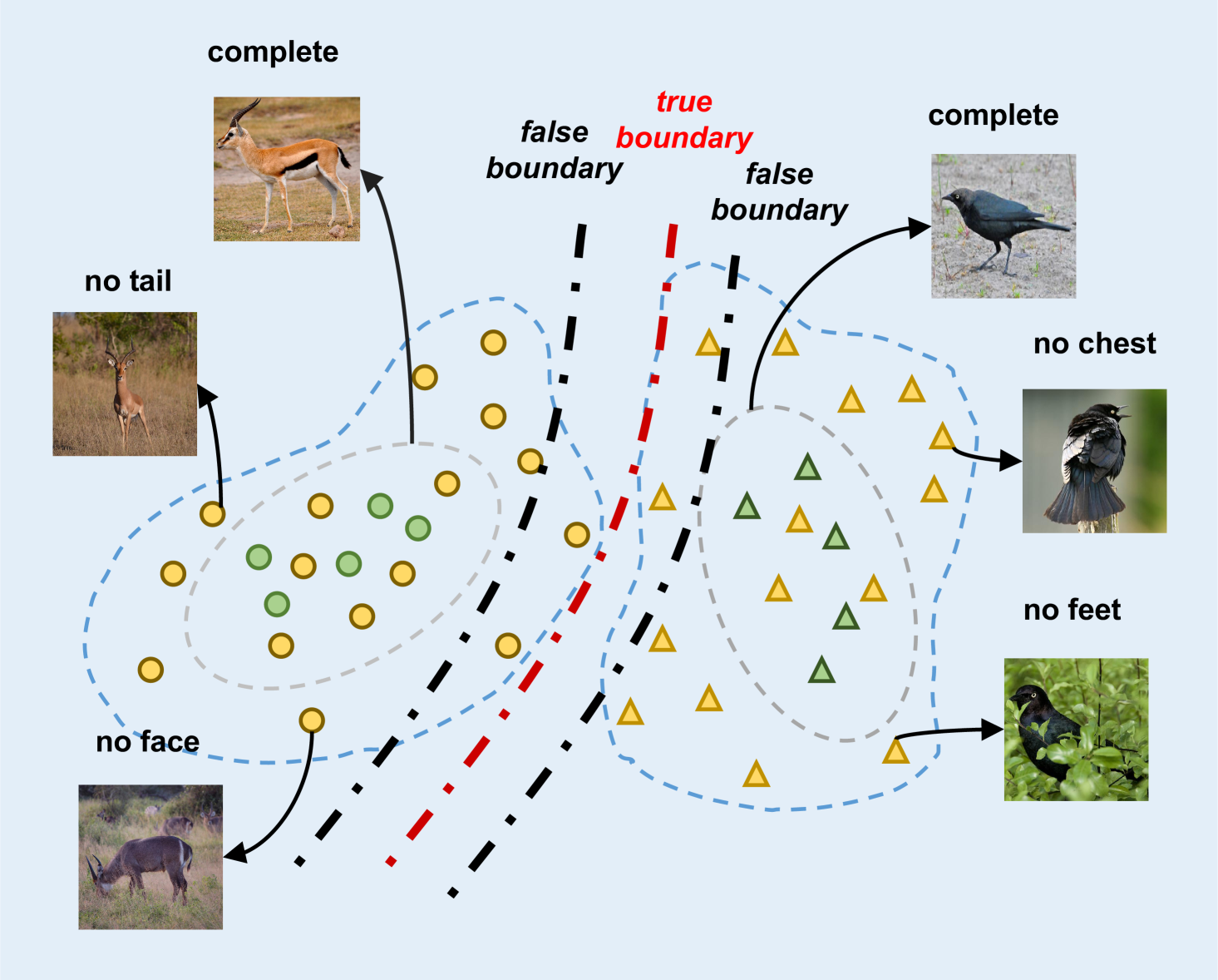
Our work mainly focuses on the generation method. When using semantic attributes to generate samples, the existing generation methods use complete semantic attributes, including all attribute information of corresponding class. Theoretically, when we generate visual features with complete semantic attributes, the generated visual features also contain complete attribute information, as depicted in Figure 1. However, the actual situation is that the visual features of categories do not always describe all the category attribute information. Let us imagine a picture of a horse in front. We cannot see the horse’s tail, so the visual features extracted from this picture must lack the characteristic information of the tail. When generating pictures, the complete semantic attributes of horses are used, and the generated visual features must be complete, which must include the characteristics of tails. It is obviously contrary and harmful to classification learning as shown in Figure 1. The classification boundary obtained from the visual features generated by a single attribute has great fluctuation, which is different from the real classification boundary, will lead to the sample being misclassified.
In order to simulate the real situation and generate a variety of visual features, so that the generated visual features contain the class-level attribute information of various situations, we propose Synthesizing Diverse Features with Attribute Augmentation (SDFA2). When generating visual features, our method better utilizes incomplete semantic attributes, which selectively masks out some bins of the semantic attributes. This simulates the absence of some attributes of visual features of real samples, so as to generate visual features closer to the real situation. Taking the semantic attribute of horse as an example, the dimension representing the tail in the semantic attribute of horse is set to 0 to represent the lack of tail attribute. The visual features of the horse generated by this incomplete semantics will also lose the attribute information of the tail. By means of this, the visual features generated by unseen classes can be closer to the real ones, and the held-out classifier trained on them observes realistic patterns, leading to better ZSL performance.
Meanwhile, the missing attribute information of visual features should be intelligible. As per our horse case, the missing tail of horse should be recognized. We add a self-monitoring module to set a Self-supervision label for each sample generated by incomplete semantic attributes to mark the missing attribute information. The generated samples are classified according to this label.
Our contributions can be described as follows:
-
•
On the basis of using complete semantic attributes to generate visual features, we propose a novel framework SDFA2 as a unified add-on to boost generative ZSL models. This method simulates the distribution of visual features in the real situation, which increases the authenticity of the generated features and improves the accuracy.
-
•
We additionally introduce self-supervised learning into our model, so that the generated visual features can be classified on the missing attributes.
-
•
We propose a general diversity feature generation method. We validate our method on two classical and two latest generative models, and the corresponding performance is improved significantly.
Related Work
Zero-Shot Learning
ZSL (Lampert, Nickisch, and Harmeling 2009; Palatucci et al. 2009) aims to transfer the model trained by the seen classes to the unseen ones, usually with a semantic space between visible classes and invisible classes. ZSL is divided into Conventional ZSL (CZSL) and generalized ZSL (GZSL). CZSL (Zhang and Saligrama 2015; Fu et al. 2015b; Xian et al. 2016; Frome et al. 2013) only contains unseen classes in the test phase while GZSL (Chao et al. 2016; Xian et al. 2018a) contains seen classes and unseen classes. GZSL has attracted more attention because it describes a more realistic scenario. In the early ZSL, the mapping method is generally used to find the relationship between visual space and semantic space. Some map visual space to semantic space (Palatucci et al. 2009; Romera-Paredes and Torr 2015). Some project visual features and semantic features into a shared space (Liu et al. 2018; Jiang et al. 2018). The others consider the mapping from the semantic space to the visual one to find classification prototypes (Annadani and Biswas 2018; Zhang, Xiang, and Gong 2017).
With the emergence of generation methods, semantic based visual feature generation Zero-Shot method also comes into being. F-CLSWGAN (Xian et al. 2018b) generates unseen visual features by generative adversarial networks. F-VAEGAN-2D (Xian et al. 2019) combines generative adversarial networks and VAE (Kingma and Welling 2014). LisGAN (Li et al. 2019) can directly generate the unseen features from random noises which are conditioned by the semantic descriptions. Cycle-CLSWGAN (Felix et al. 2018) proposes cycle consistency loss for cycle consistency detection. CE-GZSL (Han et al. 2021) adds contrastive learning for better instance-wise supervision. RFF-GZSL (Han, Fu, and Yang 2020) extracts the redundant features of the picture. ZSML (Verma, Brahma, and Rai 2020) adds Meta-Learning to the training process. IZF (Shen et al. 2020) learns factorized data embeddings with the forward pass of an invertible flow network, while the reverse pass generates data samples.
Single Attribute Problem
In the conventional ZSL setting, each category has a unified attribute, and there is a many-to-one relationship between the visual and semantic space. However, different visual features of the same category should also vary in semantic space. Based on this intuition, previous research has dealt with semantics in non generative methods. LDA (Li et al. 2018) claims that visual space may not be fully mapped to an artificially defined attribute space. Some use adaptive graph reconstruction scheme to excavate late semantics (Ding and Liu 2019). In order to avoid equal treatment of attributes, LFGAA (Liu et al. 2019) proposes a practical framework to perform object-based attribute attention for semantic disambiguation. SP-AEN (Chen et al. 2018) solves the problem of semantic attribute loss.
Most of the existing generation methods directly use the semantic attributes of the category when generating samples, and the generated visual features contain all the attribute information of the category. The reality is that some attribute features mismatch the corresponding images, and the visual features extracted by this method also have missing attributes. If we do not respect this objective fact and use the complete semantics of attribute information to generate unseen visual features with complete attribute information, the trained classification model must not be sensitive enough to those test samples with missing attribute features. Based on this fact, this paper proposes a Zero-Shot Learning method for incomplete semantic generation.
Self-Supervised Learning
Self-Supervised Learning (SSL) learns useful feature representations as a pretext to benefit the downstream tasks. Existing models deliver this with different approaches. Some methods process image color (Larsson, Maire, and Shakhnarovich 2017). Some disrupt the arrangement order after cutting pictures (Santa Cruz et al. 2017), while the others rotate images (Gidaris, Singh, and Komodakis 2018; Li et al. 2020). SSL can learn valuable representations. The purpose of our method is to use diversity attributes to generate missing features. In other words, the generated features hope to be distinguishable. Naturally, we integrate SSL into the network.
Methodology
Problem Definition
Suppose we have seen classes for training, and unseen classes that are only used for test. Let’s use and to represent seen classes space and unseen classes space, . is the visual feature of the sample in seen class, is the corresponding sample category label. Similarly, we let denotes the visual feature of the sample in unseen class, is the corresponding sample category label. At the same time, the semantic attribute of all classes is available, where denotes the seen classes attribute and is the unseen classes. In GZSL, we purpose to get a classifier , to make which is from both seen classes and unseen classes is correctly classified.
Attribute Augmentation
When generating visual features, the traditional method uses the single semantic attributes of the class, which contains all the attribute information of the class. The generation of visual features with the complete semantic attributes of the class will theoretically include all the attribute information of the class. However, the actual situation is that the visual features of some instances may not include all attribute features of this category. For example, the visual features extracted from a front picture of a antelope must not contain the attribute information of the tail, and the visual features extracted by a bird standing on a tree with its feet covered by leaves must not contain the attribute information of the talons. Then the semantic attribute corresponding to its visual features must also lack the information of tail for antelope or talons for bird.
If we use single semantic attributes when generating visual semantic features, we will not be able to simulate the visual features extracted from pictures with incomplete attributes. If all visual features are generated by using single semantic attributes, the distribution of real visual features cannot be generated. A fact is that there must be a certain number of pictures lacking complete semantic information in the sample, and there must be visual features of the sample with missing attributes. When generating unseen class visual features, if the generated visual features are complete and the test instances of unseen classes contain incomplete information, the classification results will inevitably have deviation. The classification boundary obtained by using single semantic attributes to generate visual features has a large fluctuation range and is not accurate enough. In other words, if the missing attribute information is not considered, the trained classifier will not be sensitive to the missing attribute samples. The model is not robust enough, so as to reduce the accuracy.
In order to simulate this real situation, we generate visual features with complete attribute features and missing information at the same time. For class-level semantic attribute , we artificially set dimensions to 0 to indicate the lack of attribute information. For example, the dimension of the tail in the semantic attribute of a horse is set to 0 to represent the lack of tail attribute information and the dimension of the feet in the semantic attribute of a bird is set to 0 to represent the lack of feet attribute information.
Because the semantic attribute is not marked for a specific class, but marked in the semantic space of all class, some dimensions of the semantic attribute itself are 0 for a class. Take “antelope” as an example, the dimension representing “ocean” in its semantic attribute itself is 0. Setting dimension “ocean” to 0 is meaningless and cannot represent the incomplete semantic attribute of category “antelope” without dimension “ocean”. The “grassland” attribute of antelope is not 0. “Grassland” and “ocean” are both living environments, which are semantically similar. Another example is “bipedal” and “quadrapedal” are two dimensions descriptions of semantic attributes. In fact, they are different descriptions of the same part. We know, one class cannot have both “bipedal” and “quadrapedal” attributes.Another reason is that some datasets have higher dimensions of attributes. If each dimension is set to 0 in turn, the time and space overhead will be large.
So it is harmful to set each dimension of the attribute to 0 indiscriminately. With those in mind, we believe that attributes should be grouped according to similarity. We divide the attributes by category. For each dimension description of attribute, we obtain the corresponding word vector through Word2vec (Mikolov et al. 2013) where is the number of attribute dimensions. Determine the number of clusters . Our goal is to obtain the cluster by using expectation–maximization (EM) algorithm (Anzai 2012) to minimize the square error :
| (1) |
where is the mean vector of cluster , and the calculation formula is:
| (2) |
When getting attributes divided into groups, we denote , with , as the incomplete attributes which set the i-th group attribute of semantic attribute to 0. The visual features generated in this way which uses incomplete attributes are equivalent to simulating the front picture of a horse and the picture of a bird whose feet are covered by leaves. The diversity loss can be expressed as :
| (3) |
where is the visual feature generated by and represents the loss function related to visual features and represents the loss function related to semantic attributes in generative network. Take WGAN as an example, the diversity losses can be expressed as:
| (4) |
where is the semantic attribute with , is the generated visual feature with , is obtained from . The last one is the gradient penalty, where with and is the penalty coefficient.
| AWA | CUB | aPY | SUN | |||||||||
|---|---|---|---|---|---|---|---|---|---|---|---|---|
| U | S | H | U | S | H | U | S | H | U | S | H | |
| f-CLSWGAN (Xian et al. 2018b) | 57.9 | 61.4 | 59.6 | 43.7 | 57.7 | 49.7 | 32.9 | 61.7 | 42.9 | 42.6 | 36.6 | 39.4 |
| f-CLSWGAN+SDFA2 | 59.1 | 72.8 | 65.2 | 51.5 | 57.5 | 54.3 | 38.0 | 62.8 | 47.4 | 48.7 | 36.9 | 42.0 |
| f-VAEGAN-D2 (Xian et al. 2019) | 59.7 | 68.1 | 63.7 | 51.7 | 55.3 | 53.5 | 29.1 | 60.4 | 39.2 | 48.6 | 36.7 | 41.8 |
| f-VAEGAN-D2+SDFA2 | 59.5 | 71.4 | 64.7 | 53.3 | 55.0 | 54.2 | 39.4 | 57.5 | 46.8 | 48.5 | 37.6 | 42.4 |
| RFF-GZSL (Han, Fu, and Yang 2020) | 49.7 | 50.8 | 61.5 | 52.1 | 57.0 | 54.4 | 18.6 | 86.7 | 30.6 | 42.7 | 37.4 | 39.9 |
| RFF-GZSL+SDFA2 | 57.0 | 75.5 | 65.0 | 52.3 | 57.4 | 54.7 | 27.4 | 66.9 | 38.9 | 42.9 | 51.6 | 40.1 |
| CE-GZSL (Han et al. 2021) | 57.0 | 74.9 | 64.7 | 49.0 | 57.4 | 53.0 | 9.58 | 88.4 | 17.3 | 40.9 | 35.4 | 37.9 |
| CE-GZSL+SDFA2 | 59.3 | 75.0 | 66.2 | 59.2 | 59.6 | 54.0 | 21.5 | 85.1 | 34.3 | 46.2 | 32.6 | 38.2 |
Self-Supervision of Missing Attributes
The visual features of real instances can distinguish the missing semantic attributes, that is, the visual features extracted from the front picture of the horse can distinguish the missing tail attribute. Similarly, the visual features extracted from a picture of a bird whose feet are covered by leaves can identify the absence of feet attributes.
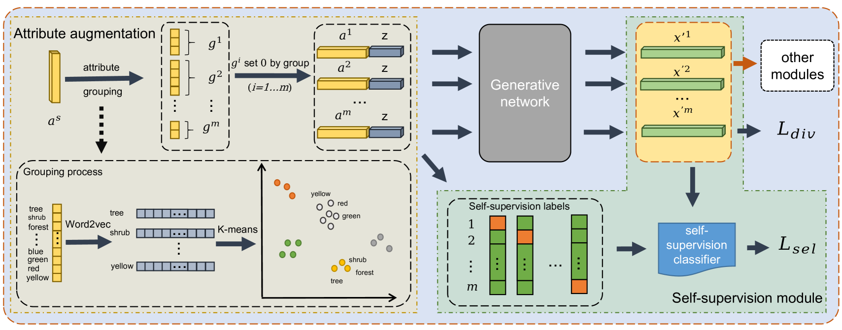
In order to make the visual features generated by diversity attributes more in line with the real situation, in other words, we can judge the missing attribute information of the generated visual features, we introduce self-supervision loss, As shown in Figure 2. For the incomplete semantic attribute whose i-th group attribute is set to 0, we set a Self-supervision label for the generated , to denote the visual features generated missing the attributes of the i-th group. Note that represents visual features generated using complete semantic attributes .
For each incompletely generated sample, we train a mapping relation , where is a learnable incomplete attribute recognition classifier with . So the diversity identification loss is:
| (5) |
Total Loss
Finally, according to the Eq.(3) and Eq.(5), diverse feature synthesis method consists of the loss of diversity semantic generation and the loss of missing attribute self-supervision. The total loss of our model is:
| (6) |
where and are hyper-parameters.
Figure 2 is the overall framework of our method. Among them, generator and discriminator of generative network can be replaced with different types. Other modules are additional contents added outside the main body of the generated network, such as classification loss in f-CLSWGAN, contrast loss in CE-GZSL, etc. Our method is a general module, which can be added to any ZSL that uses attributes to generate visual features.
Training Classifier
Compared with traditional method which only uses a single semantic attribute when generating visual features, our method additional uses the semantic attribute of attribute dimension grouped and setted 0 when generating visual features. Specifically, compared with the number of visual feature generation using a single semantic attribute, we generate visual features for each diverse semantic attribute in a certain proportion. We use the visual feature generated by single semantic attribute and the visual feature generated by diversity semantic attribute, which denotes , to train the classifier together with the visual feature .
Experiments
Datasets Introduction and Setting
We evaluated our method on four data sets, i.e., AWA1 (Lampert, Nickisch, and Harmeling 2009) containing 50 animal category attribute descriptions; CUB (Welinder et al. 2010) is a fine-grained data set about birds; SUN (Patterson et al. 2014) is a fine-grained data set about visual scenes; Attribute Pascal and Yahoo are abbreviated as aPY (Farhadi et al. 2009). Table 2 shows the number division of seen and unseen classes, attribute dimensions and number of samples of the four data sets. All data sets extract visual features of 2048 dimensions through ResNet-101 (He et al. 2016) without finetuning. The semantic attributes of the four data sets adopt the original semantic attributes.
We implement the proposed method on PyToch. We use a layer of network with Sigmod activation function for Self-supervision classifier. After training the generation network, for the visual features generated by unseen classes, on the basis of using a single category attribute, we use the incomplete semantic attributes of classes to generate some visual features in proportion. At the same time, the visual features generated by our generation network are more diversified. In order to prevent over fitting of the generation network, we add L2 regularization to the optimizer of the generation network.
| Datasets | Seen | Unseen | Attribute | Samples |
|---|---|---|---|---|
| AWA | 40 | 10 | 85 | 30,475 |
| aPY | 20 | 12 | 64 | 15,339 |
| CUB | 150 | 50 | 312 | 11,788 |
| SUN | 645 | 72 | 102 | 14,340 |
Evaluation Protocols
We follow the evaluation method proposed by harmonic average (Xian et al. 2018a). For GZSL, we calculate the average accuracy and of seen and unseen classes respectively. The performance of GZSL is evaluated by their harmonic average: .
Improvement against Existing Methods
In order to verify that our incomplete generation method is a general method, we add our generation method based on the models of f-WGAN, f-VAEGAN-D2, RFF-GZSL and CE-GZSL.
For f-CLSWGAN, a single attribute is used to generate features and calculate generative adversarial loss and classification loss. On this basis, after using our method to generate diversity features, we need to calculate not only the corresponding generative adversarial loss, but also the loss of the generated diversity features on the pre trained classifier.
For f-VAEGAN-2D, the original model is divided into VAE and WGAN. SDFA2 only modifies WGAN module. On the basis of the original single attribute generation feature, which produces the generative adversarial loss, increases the generative adversarial loss caused by using the diversity generation feature.
For RFF-GZSL, the additional features generated by our method also need to go through mapping function to transform the diversity visual features to the redundancy free features, and then calculate the corresponding loss. Similarly, the original model adopts the classification loss in f-CLSWGAN, and the diversity features we generate also need to calculate the classification loss.
For CE-GZSL, the additional generated diversity visual features need to go through the embedding function proposed by the original model, and the corresponding loss is calculated through two modules: instance-level contrast embedding and class-level contrast embedding.
Parameter Setting
Due to the different experimental equipment and parameter settings, which most important thing is that we only have one GTX 1080ti GPU, it is difficult to restore the test results given by some generation models. However, we just want to verify that our method is a general method for generating class model, so we use the method of controlling variables.
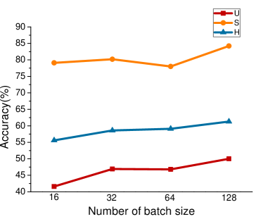
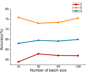
For RFF-GZSL, we change the batch size. We set batch size to 128 on all four data sets. At the same time, for the fine-grained data sets SUN and CUB, we use the original attributes. Other parameters refer to the values given in the paper. For CE-GZSL, we hope to use the batch size provided in the paper, but the model is too complex and limited by equipment. We also set batch size to 128, which will have a certain impact on the comparative learning module in CE-GZSL. Other parameter settings follow the values given in the paper. In order to prove the influence of different batch sizes on the experimental results, we set different batch sizes on RFF-GZSL. The results are shown in Figure 4, we can clearly see that is increasing with the increase of batch size.
On the basis of following the parameters given by these three models, we obtain the operation results on our equipment. Then, we fix all the parameters of the model without changing, and add our proposed method. The experiment in this section is not to compare with the state-of-the-art methods, but to verify that the general method proposed by us is universal in improving the effect of the generated model. The experimental results are shown in table 1.
Comparison and Evaluation
It can be seen that our method has significantly improved the effect of the three generation methods. Especially on the AWA1 and aPY data sets, the improvement effect is obvious. See the f-CLSWGAN with SDFA2, the AWA1 is increased by 5.6 percentage points, and the aPY is increased by 4.5 percentage points. On f-AVEGAN-D2, after using SDFA2, the H of AWA1 is 64.7% and aPY is 46.8%. After using SDFA2, CE-GZSL and RFF-GZSL increased by 1.5% and 3.5% respectively for AWA1, and increased by 17% and 8.3% respectively for aPY. It can be seen that the features of generating diversity contribute to the improvement of performance.
For the fine-grained data sets SUN and CUB, because the gap between classes is subtle, the gap between categories becomes smaller after masking a feature to 0, so the effect improvement is not as significant as AWA1 and aPY. However, the improvement in f-CLSWGAN and f-AVEGAN is still significant, reaching 42.0% and 42.4% in SUN, 54.2% and 54.2% in CUB respectively. There are also some improvements in CE-GZSL and RFF-GZSL.
| AWA1 | aPY | SUN | CUB | |||||||||
|---|---|---|---|---|---|---|---|---|---|---|---|---|
| U | S | H | U | S | H | U | S | H | U | S | H | |
| f-CSLWGAN+ | 58.9 | 71.3 | 64.5 | 37.0 | 64.7 | 47.1 | 47.2 | 35.4 | 40.5 | 51.7 | 56.7 | 54.1 |
| f-CLSWGAN++ | 59.1 | 72.8 | 65.2 | 38.0 | 62.8 | 47.4 | 48.7 | 36.9 | 42.0 | 51.5 | 57.5 | 54.3 |
Number of Attribute Groups
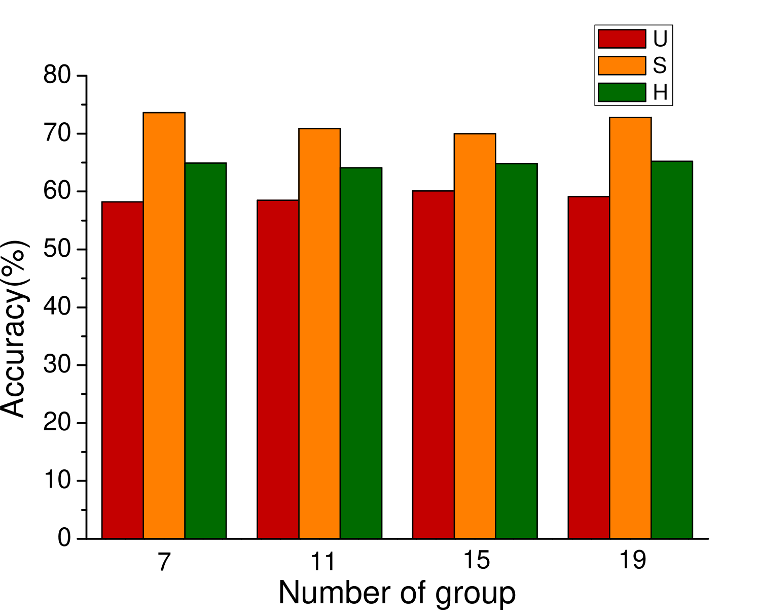
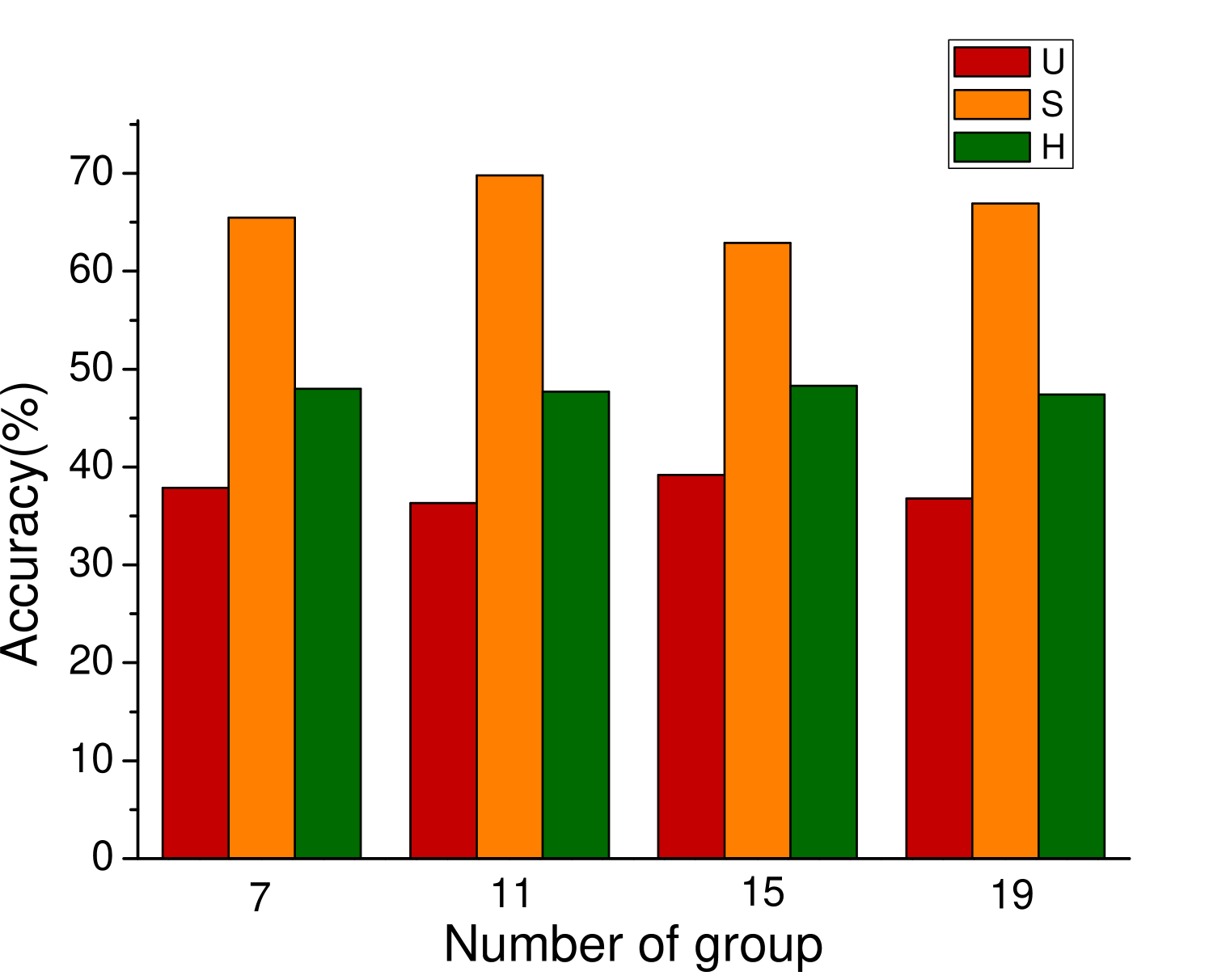
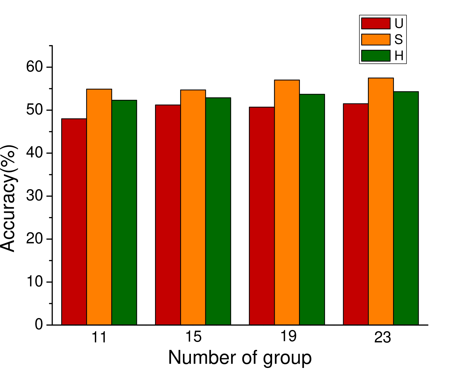
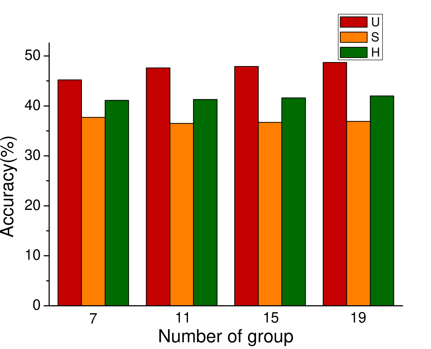
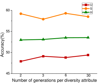
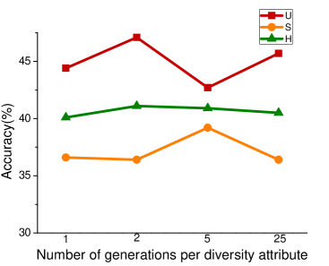
In the process of attribute grouping, the selection of the number of groups, in other words, the selection of the number of cluster centers is a problem to be considered. The choice of different number of cluster centers will have different effects on the final results. In order to test the influence of attribute grouping on diversity generation, we set up different number of clustering centers in the process of attribute clustering. Figure 3 shows the results of different data sets based on f-CLSWGAN with SDFA2 after setting different clustering centers. We can clearly see that the number of different attribute groups has little effect on the performance of the model.
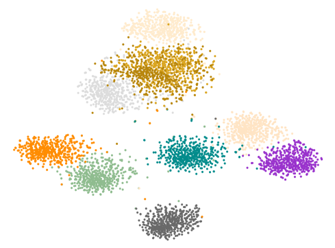
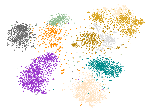

Diversity Generation
The main purpose of our proposed SDFA2 is to generate visual features through diversity attributes. Different from the method of generating visual features using a single attribute, which only increases diversity through Gaussian noise. Figure 5 (a) shows the results of the visual features generated by the traditional single attribute generation method under t-SNE. It can be seen that the generated visual features show an obvious Gaussian distribution. Figure 5 (b) shows the features distribution of samples of real unseen classes. Figure 5 (c) is the result of visual features generated by the generation network trained using SDFA2 method under t-SNE. Obviously, it is more in line with the real distribution. So, the generated samples can better replace the real samples for classifier training.
Ablation Experiment
In order to verify the impact of incomplete generation method and self supervised classification loss on the performance of the model, we designed ablation experiments. We first increase only diversity loss, then add diversity loss and self-supervision loss at the same time. The experimental results are shown in Table 3. It can be seen that incomplete loss and self-monitoring loss significantly improve the performance of the model.
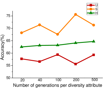
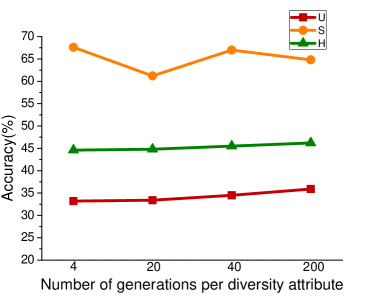
Numbers of Synthesized Features
The number of diversity generation is an important parameter in our method. In order to explore the impact of different generation quantities on the performance of the model, we designed this experiment. We fixed the number of visual features generated by a single attribute for each class, AWA1 with 2000, aPY with 2000, CUB with 300 and SUN with 50. Then, according to different proportions, the diversity attribute is used to generate additional visual features. Figure 6 shows the results of four data sets at different scales. It is obvious that there are significant differences in the results under different proportions. This is because in the real situation, there is a certain relationship between the number of pictures with complete attributes and the number of pictures with incomplete attributes, so the number of generated pictures with different proportions will inevitably have a certain impact on the results.
Conclusion
In this work, we propose an attribute enhancement method to generate diversity features, which is used to drive the generated feature distribution to approach the real feature distribution. We solve the problem that the attribute features used in the existing generative GZSL methods are too single. At the same time, based on diversity feature generation, a self-supervision loss is proposed to enhance visual feature generation. Experiments show that our SDFA2 has good generality on different generative GZSL models. Considering that attribute mask is not the only way to generate diversity attributes, we will do more processing on attributes in external work in order to generate visual features more in line with the real distribution.
Acknowledgments
This work was supported in part by the National Natural Science Foundation of China (NSFC) under Grants No. 61872187, No. 62077023 and No. 62072246, in part by the Natural Science Foundation of Jiangsu Province under Grant No. BK20201306, and in part by the “111 Program” under Grant No. B13022.
References
- Annadani and Biswas (2018) Annadani, Y.; and Biswas, S. 2018. Preserving semantic relations for zero-shot learning. In CVPR, 7603–7612.
- Anzai (2012) Anzai, Y. 2012. Pattern recognition and machine learning. Elsevier.
- Bucher, Herbin, and Jurie (2016) Bucher, M.; Herbin, S.; and Jurie, F. 2016. Improving semantic embedding consistency by metric learning for zero-shot classiffication. In ECCV, 730–746.
- Cacheux, Borgne, and Crucianu (2019) Cacheux, Y. L.; Borgne, H. L.; and Crucianu, M. 2019. Modeling inter and intra-class relations in the triplet loss for zero-shot learning. In ICCV, 10333–10342.
- Chao et al. (2016) Chao, W.-L.; Changpinyo, S.; Gong, B.; and Sha, F. 2016. An empirical study and analysis of generalized zero-shot learning for object recognition in the wild. In ECCV, 52–68.
- Chen et al. (2018) Chen, L.; Zhang, H.; Xiao, J.; Liu, W.; and Chang, S.-F. 2018. Zero-shot visual recognition using semantics-preserving adversarial embedding networks. In CVPR, 1043–1052.
- Ding and Liu (2019) Ding, Z.; and Liu, H. 2019. Marginalized latent semantic encoder for zero-shot learning. In CVPR, 6191–6199.
- Farhadi et al. (2009) Farhadi, A.; Endres, I.; Hoiem, D.; and Forsyth, D. 2009. Describing objects by their attributes. In CVPR, 1778–1785.
- Felix et al. (2018) Felix, R.; Reid, I.; Carneiro, G.; et al. 2018. Multi-modal cycle-consistent generalized zero-shot learning. In ECCV, 21–37.
- Frome et al. (2013) Frome, A.; Corrado, G. S.; Shlens, J.; Bengio, S.; Dean, J.; Ranzato, M. A.; and Mikolov, T. 2013. DeViSE: a deep visual-semantic embedding model. In NeurIPS.
- Fu et al. (2015a) Fu, Y.; Hospedales, T. M.; Xiang, T.; and Gong, S. 2015a. Transductive multi-view zero-shot learning. IEEE TPAMI, 37(11): 2332–2345.
- Fu et al. (2015b) Fu, Z.; Xiang, T.; Kodirov, E.; and Gong, S. 2015b. Zero-shot object recognition by semantic manifold distance. In CVPR, 2635–2644.
- Gidaris, Singh, and Komodakis (2018) Gidaris, S.; Singh, P.; and Komodakis, N. 2018. Unsupervised representation learning by predicting image rotations. In ICLR.
- Han et al. (2021) Han, Z.; Fu, Z.; Chen, S.; and Yang, J. 2021. Contrastive embedding for generalized zero-shot learning. In CVPR, 2371–2381.
- Han, Fu, and Yang (2020) Han, Z.; Fu, Z.; and Yang, J. 2020. Learning the redundancy-free features for generalized zero-shot object recognition. In CVPR, 12865–12874.
- He et al. (2016) He, K.; Zhang, X.; Ren, S.; and Sun, J. 2016. Deep residual learning for image recognition. In CVPR, 770–778.
- Jiang et al. (2018) Jiang, H.; Wang, R.; Shan, S.; and Chen, X. 2018. Learning class prototypes via structure alignment for zero-shot recognition. In ECCV, 118–134.
- Kingma and Welling (2014) Kingma, D. P.; and Welling, M. 2014. Auto-encoding variational bayes. In ICLR.
- Kodirov, Xiang, and Gong (2017) Kodirov, E.; Xiang, T.; and Gong, S. 2017. Semantic autoencoder for zero-shot learning. In CVPR, 3174–3183.
- Lampert, Nickisch, and Harmeling (2009) Lampert, C. H.; Nickisch, H.; and Harmeling, S. 2009. Learning to detect unseen object classes by between-class attribute transfer. In CVPR, 951–958.
- Larsson, Maire, and Shakhnarovich (2017) Larsson, G.; Maire, M.; and Shakhnarovich, G. 2017. Colorization as a proxy task for visual understanding. In CVPR, 6874–6883.
- Li et al. (2019) Li, J.; Jing, M.; Lu, K.; Ding, Z.; Zhu, L.; and Huang, Z. 2019. Leveraging the invariant side of generative zero-shot learning. In CVPR, 7402–7411.
- Li et al. (2020) Li, Y.; Xu, H.; Zhao, T.; and Fang, E. X. 2020. Implicit bias of gradient descent based adversarial training on separable data. In ICLR.
- Li et al. (2018) Li, Y.; Zhang, J.; Zhang, J.; and Huang, K. 2018. Discriminative learning of latent features for zero-shot recognition. In CVPR, 7463–7471.
- Liu et al. (2018) Liu, S.; Long, M.; Wang, J.; and Jordan, M. I. 2018. Generalized zero-shot learning with deep calibration network. In NeurIPS, 2005–2015.
- Liu et al. (2019) Liu, Y.; Guo, J.; Cai, D.; and He, X. 2019. Attribute attention for semantic disambiguation in zero-shot learning. In ICCV, 6698–6707.
- Mikolov et al. (2013) Mikolov, T.; Chen, K.; Corrado, G.; and Dean, J. 2013. Efficient estimation of word representations in vector space. In ICLR Workshop.
- Narayan et al. (2020) Narayan, S.; Gupta, A.; Khan, F. S.; Snoek, C. G.; and Shao, L. 2020. Latent embedding feedback and discriminative features for zero-shot classification. In ECCV, 479–495.
- Palatucci et al. (2009) Palatucci, M. M.; Pomerleau, D. A.; Hinton, G. E.; and Mitchell, T. 2009. Zero-shot learning with semantic output codes. In NeurIPS.
- Patterson et al. (2014) Patterson, G.; Xu, C.; Su, H.; and Hays, J. 2014. The sun attribute database: Beyond categories for deeper scene understanding. IJCV, 108(1-2): 59–81.
- Romera-Paredes and Torr (2015) Romera-Paredes, B.; and Torr, P. 2015. An embarrassingly simple approach to zero-shot learning. In ICML, 2152–2161.
- Santa Cruz et al. (2017) Santa Cruz, R.; Fernando, B.; Cherian, A.; and Gould, S. 2017. Deeppermnet: Visual permutation learning. In CVPR, 3949–3957.
- Shen et al. (2020) Shen, Y.; Qin, J.; Huang, L.; Liu, L.; Zhu, F.; and Shao, L. 2020. Invertible zero-shot recognition flows. In ECCV, 614–631.
- Sun et al. (2020) Sun, L.; Song, J.; Wang, Y.; and Li, B. 2020. Cooperative coupled generative networks for generalized zero-shot learning. IEEE Access, 8: 119287–119299.
- Verma, Brahma, and Rai (2020) Verma, V. K.; Brahma, D.; and Rai, P. 2020. Meta-learning for generalized zero-shot learning. In AAAI, 6062–6069.
- Wang et al. (2018) Wang, W.; Pu, Y.; Verma, V. K.; Fan, K.; Zhang, Y.; Chen, C.; Rai, P.; and Carin, L. 2018. Zero-shot learning via class-conditioned deep generative models. In AAAI.
- Welinder et al. (2010) Welinder, P.; Branson, S.; Mita, T.; Wah, C.; Schroff, F.; Belongie, S.; and Perona, P. 2010. Caltech-UCSD birds 200. Technical report, California Institute of Technology.
- Xian et al. (2016) Xian, Y.; Akata, Z.; Sharma, G.; Nguyen, Q.; Hein, M.; and Schiele, B. 2016. Latent embeddings for zero-shot classification. In CVPR, 69–77.
- Xian et al. (2018a) Xian, Y.; Lampert, C. H.; Schiele, B.; and Akata, Z. 2018a. Zero-shot learning—a comprehensive evaluation of the good, the bad and the ugly. IEEE TPAMI, 41(9): 2251–2265.
- Xian et al. (2018b) Xian, Y.; Lorenz, T.; Schiele, B.; and Akata, Z. 2018b. Feature generating networks for zero-shot learning. In CVPR, 5542–5551.
- Xian et al. (2019) Xian, Y.; Sharma, S.; Schiele, B.; and Akata, Z. 2019. f-vaegan-d2: A feature generating framework for any-shot learning. In CVPR, 10275–10284.
- Yu et al. (2020) Yu, Y.; Ji, Z.; Han, J.; and Zhang, Z. 2020. Episode-based prototype generating network for zero-shot learning. In CVPR, 14035–14044.
- Zhang et al. (2018) Zhang, H.; Long, Y.; Guan, Y.; and Shao, L. 2018. Triple verification network for generalized zero-shot learning. IEEE TIP, 28(1): 506–517.
- Zhang et al. (2019) Zhang, H.; Mao, H.; Long, Y.; Yang, W.; and Shao, L. 2019. A probabilistic zero-shot learning method via latent nonnegative prototype synthesis of unseen classes. IEEE TNNLS, 31(7): 2361–2375.
- Zhang, Xiang, and Gong (2017) Zhang, L.; Xiang, T.; and Gong, S. 2017. Learning a deep embedding model for zero-shot learning. In CVPR, 2021–2030.
- Zhang and Saligrama (2015) Zhang, Z.; and Saligrama, V. 2015. Zero-shot learning via semantic similarity embedding. In ICCV, 4166–4174.