Bootstrapping Adaptive Human-Machine Interfaces
with Offline Reinforcement Learning
Abstract
Adaptive interfaces can help users perform sequential decision-making tasks like robotic teleoperation given noisy, high-dimensional command signals (e.g., from a brain-computer interface). Recent advances in human-in-the-loop machine learning enable such systems to improve by interacting with users, but tend to be limited by the amount of data that they can collect from individual users in practice. In this paper, we propose a reinforcement learning algorithm to address this by training an interface to map raw command signals to actions using a combination of offline pre-training and online fine-tuning. To address the challenges posed by noisy command signals and sparse rewards, we develop a novel method for representing and inferring the user’s long-term intent for a given trajectory. We primarily evaluate our method’s ability to assist users who can only communicate through noisy, high-dimensional input channels through a user study in which 12 participants performed a simulated navigation task by using their eye gaze to modulate a 128-dimensional command signal from their webcam. The results show that our method enables successful goal navigation more often than a baseline directional interface, by learning to denoise user commands signals and provide shared autonomy assistance. We further evaluate on a simulated Sawyer pushing task with eye gaze control, and the Lunar Lander game with simulated user commands, and find that our method improves over baseline interfaces in these domains as well. Extensive ablation experiments with simulated user commands empirically motivate each component of our method.
I Introduction
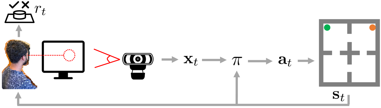
One of the central problems in the field of human-computer interaction is designing interfaces that help users control complex systems, such as prosthetic limbs and assistive robots, by translating raw user commands (e.g., brain signals) into actions (illustrated in Fig. 1). Recent work proposes various human-in-the-loop reinforcement learning (RL) algorithms that address this challenge by training the interface to maximize positive user feedback on the system’s performance [1, 2, 3, 4, 5, 6, 7]. This approach customizes the interface to individual users and improves with use, but tends to require a large amount of human interaction data. Prior work improves data efficiency by assuming access to some combination of the user’s task distribution, a task-agnostic reward function, and a prior mapping from raw user commands into actions [3, 6, 7], which can be difficult to specify in practice. In this paper, we lift these assumptions using recent advances in offline RL [8, 9, 10, 11, 12, 13, 14, 15], to instead leverage offline data for improved online data efficiency.
Instead of assuming prior knowledge of the user’s desired tasks, we take a purely data-driven approach to interface optimization. We propose an offline RL algorithm for interface optimization that can learn from both an observational dataset of the user attempting to perform their desired tasks using some unknown existing default interface, as well as online data collected using our learned interface, where each episode is labeled with a sparse reward that indicates overall task success or failure. We assume that the default interface is performant enough for the user to produce data that contains useful behavior to learn from. To address the high cost of user data, we pre-train value functions on a large offline dataset, and distill them into a policy (i.e., an interface) that infers the user’s desired action from the user’s command signal. To enable the user and interface to co-adapt and discover command styles that are different from those in the offline data, we then fine-tune the interface through online, human-in-the-loop RL. In our experiments, we instantiate this approach with implicit Q-learning (IQL) [16]. We call our method the Offline RL-Bootstrapped InTerface (ORBIT).
There are several challenging features of our problem setting that resist straightforward applications of existing offline RL algorithms. First, the user’s command is noisy and only provides a partial observation of the user’s long-term intent. Second, we assume that users can only provide sparse, terminal rewards, as more complex forms of reward feedback can be difficult to specify in practice. These factors, combined with practical limitations on the size of the offline dataset, makes learning a representation of the user’s intent challenging. As such, we train representations of user intent to be predictive of the user’s rewards, which we use to condition our offline RL algorithm on. To avoid overfitting, we propose to regularize these learned representations using negative data augmentation and a variational information bottleneck.
Our setting also differs from the standard offline RL regime in that, during online fine-tuning, the user can adapt to the interface to operate it more effectively. While this can make RL more difficult due to non-stationary dynamics, it also presents an opportunity to learn an interface that not only denoises commands and autocompletes actions, but departs from the overall command strategy of the default interface and the offline data.
To our knowledge, ORBIT is the first human-in-the-loop RL algorithm that can learn an interface from both offline and online data. One key improvement over prior work is a novel representation learning method for encoding and conditioning on full trajectories in the value function (Sec. II-A), and for conditioning on the history of previous states and commands in the policy (Sec. II-B). To evaluate ORBIT’s ability to learn an effective interface from real user data, we conduct a user study with 12 participants who perform a simulated navigation task by using their eye gaze to modulate a 128-dimensional command signal from their webcam (illustrated in Fig. 3 and 5). The results show that ORBIT enables the user to successfully navigate to their goal more often than a default, directional interface used to collect the training data. We also showcase ORBIT on a simulated Sawyer pushing task with input from a single human user, and on the Lunar Lander game with simulated user input (see Table II).
II Interface Optimization via Offline RL
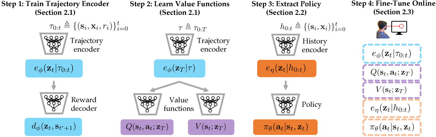
In our setting, the user cannot directly take actions, and relies on an interface to convert the user’s raw command signals into actions. The interface cannot directly observe any specification of the desired task. We formulate the assistance problem as a contextual Markov decision process (CMDP) [17]. Each observation consists of two variables: the state of the environment (e.g., the position of the robot) and the user’s command (e.g., brain signals). The interface takes an action given a history of previous states and commands . We do not assume that we can observe the user’s desired task (which defines the context in the CMDP), the space of possible tasks, or the ground-truth reward function . Instead, we assume access to a reward signal that comes from the user—to simplify our method and experiments, we assume that the user only provides a binary reward at the end of each episode to indicate whether the interface succeeded or failed at the user’s desired task, and automatically set non-terminal rewards to zero. We approach this problem by using offline RL and online fine-tuning to train an interface to maximize the user-provided rewards. Fig. 2 outlines our method.
II-A Learning Value Functions from Partial Observations
In order to train an effective interface, we would like to learn the action-value function and state-value function from an offline dataset of trajectories in which the user gives commands, some unknown default interface executes actions, and the user gives reward feedback. However, the user’s commands only provide partial observations of the user’s long-term intent. To accurately model the value function, we represent the user’s intent as a function of the full sequence of observed environment states and corresponding commands. To accomplish this, we learn a trajectory encoder that takes in a sequence of tuples , denoted as a partial trajectory , and outputs a distribution over the latent embedding that represents the user’s intent (see Step 1 in Fig. 2). Note that this trajectory encoder also takes rewards as input, since rewards contain important information about the user’s intent in retrospect. We then condition both value functions and on a latent embedding of the full trajectory that the input comes from, where denotes the mean embedding .
To ensure that the latents contain information about the user’s intent, we train the trajectory encoder such that the latents are predictive of the user’s reward labels, akin to prior work [18]. In particular, we train end to end with a reward decoder that predicts the reward given the pair for any (including ). For the reward decoder to accurately predict the reward for entering the state , the latent must contain information about the user’s desired task inferred from the partial trajectory . We jointly train the trajectory encoder and the reward decoder to minimize the reward prediction error,
| (1) |
where is the cross entropy, and is an offline dataset of trajectories. The ablation experiment for Q8 in Sec. V shows that training the trajectory encoder to predict rewards performs much better than end to end with the value functions.
The purpose of the reward decoder is to force the latent to contain useful information about the user’s intent, but without any regularization, it learns to accurately predict the reward based on the state alone while ignoring the latent , causing the trajectory encoder to generate uninformative latents. The ablation experiment for Q4 in Sec. V shows that this effect substantially degrades the performance of the interface. To encourage the reward decoder to use the latent to predict the reward , we also train on an auxiliary loss term that mimics the binary cross-entropy loss in Eqn. 1, but pairs the states from trajectory with the latents from a different trajectory , and labels the resulting pairs with zero rewards . We refer to this term as the negative data augmentation loss,
| (2) |
where the trajectory is randomly sampled from the dataset , and belongs to the trajectory . To prevent the reward decoder from overfitting to embeddings of the offline trajectories, we regularize the upstream trajectory encoder with a variational information bottleneck (VIB) [19, 20],
| (3) |
where is the dimensionality of the latent space. The ablation experiment for Q5 in Sec. V shows that this VIB is critical to the empirical performance of the interface.
Putting the reward prediction error, negative data augmentation, and information bottleneck losses together, we have
| (4) |
where is a constant hyperparameter. In our experiments, we model the trajectory encoder as a gated recurrent neural network (RNN) [21], and the reward decoder as a feedforward neural network. After training to minimize the loss in Eqn. 4, we fit the value functions and by optimizing the value losses and from implicit Q-learning (IQL) [16].
While we intend for the trajectory encoder to help address the challenges of estimating user intent from sparse rewards, it does not directly address the more general exploration and optimization challenges of RL with sparse rewards, which is outside the scope of this work.
II-B Extracting a Policy from the Value Functions
We would like to train a policy to maximize the learned values. Due to the partial observability of the user’s long-term intent given their commands, this policy should be conditioned on the history of previous states and commands. We could simply reuse the learned trajectory encoder from the previous section to embed this history, along with rewards set to zero, as is trained to produce latents informative of user intent from this input. However, the ablation experiment for Q6 in Sec. V shows that this performs substantially worse than baseline methods.
Instead, we train a new ‘history encoder’ that takes a history as input, and outputs a distribution over the latent embedding . Using this history encoder, we model the policy as , where denotes the mean embedding . We train the policy and history encoder on the weighted behavioral cloning (BC) loss from [22],
| (5) |
where is a constant hyperparameter, the weights are the exponentiated advantages , and and are the value functions learned through IQL in Sec. II-A. Note that the policy is conditioned on the embedding from the history encoder , while the advantages are obtained by conditioning on the full trajectory embedding from the trajectory encoder . Step 3 in Fig. 2 illustrates this policy architecture in relation to our overall method.
As with the trajectory encoder, we regularize the history encoder using a VIB—the ablation experiment for Q5 in Sec. V shows that this is critical for performance. Putting the weighted BC and VIB losses together, we have the policy extraction loss,
| (6) |
where is a constant hyperparameter, and is analogous to Eqn. 3. In our experiments, we model the policy as a feedforward network, and the history encoder as a permutation-invariant product of independent Gaussian factors similar to prior work [23]. We use this architecture for the history encoder, instead of an RNN like the trajectory encoder, because while the trajectory encoder is only evaluated in-distribution, the history encoder is evaluated during online rollouts, where there can be distribution shift. Thus, it benefits from the regularization of a permutation-invariant architecture.
In summary, the history encoder differs from the trajectory encoder in the following ways: 1. It is used to condition the policy. 2. It is only conditioned on past histories, because this is what is available during online rollouts. 3. It is trained end to end with the weighted BC objective. 4. It uses a permutation-invariant architecture for greater regularization.
II-C Online Fine-Tuning
The previous sections describe how to pre-train a policy on an offline dataset . However, pre-training alone may not outperform the default interface used to generate the offline data. To address this issue, we have the user operate the pre-trained interface, and further optimize it through online RL. Fine-tuning the interface with the user in the loop generates on-policy training data and explores new interfaces.
During the online fine-tuning phase, we update the value functions, which first involves updating the learned representations of the user’s intent. To do so, we update the trajectory encoder by taking gradient steps on the loss in Eqn. 4 after each episode. To reduce variance in the learning signal, we remove negative data augmentation—augmentation is not required because the decoder has already learned to use the latent for reward prediction during the offline learning phase. To further stabilize fine-tuning of the trajectory encoder , we also implement a trust region loss that keeps the fine-tuned trajectory encoder close to the pre-trained (and frozen) trajectory encoder: we freeze the reward decoder and pre-trained trajectory encoder , and minimize the KL divergence between the fine-tuned trajectory encoder and the pre-trained trajectory encoder on the offline data ,
| (7) |
We then update the value functions and by taking gradient steps on the value losses from IQL ( and in [16]). Finally, we update the policy and history encoder by taking gradient steps on the loss in Eqn. 6. To prevent catastrophic forgetting, each mini-batch of trajectories is balanced to consist of 50% offline and 50% online data. While the offline data may include lower quality samples, using offline RL should help address learning from suboptimal data.
Algorithm 1 outlines the full method, which we call the Offline RL-Bootstrapped InTerface (ORBIT). We first take an offline dataset of trajectories labeled with sparse rewards, and learn a trajectory encoder , value functions and , reward decoder , history encoder , and policy (see Fig. 2 for an overview). We then fine-tune these models (except the reward decoder) on online trajectories collected with the user as they operate the learned interface .
III Related Work
The literature on learning-based assistive interfaces spans several fields, including brain-computer interfaces [24, 25, 26, 27, 28, 29], natural language interfaces [30, 31, 32], speech interfaces [33, 34], electronic musical instruments [35], and robotic teleoperation interfaces [36, 37, 38, 39, 40, 41]. This prior work assumes access to some combination of a user model, candidate tasks, and ground-truth action labels for commands, which restricts them to settings with substantial prior knowledge or supervision. Recent work on human-in-the-loop RL [3, 6, 7] lifts these assumptions, but still assumes access to either a task-agnostic reward function, task distribution, or prior interface. In contrast, ORBIT only assumes access to a dataset of trajectories where the user provided a command, the system took an action, and the user provided a sparse reward signal. This purely data-driven approach to interface optimization makes ORBIT more practical for a broad range of real-world applications, where users can easily generate trajectory data but cannot manually specify their task distribution or a prior mapping. While the performance of ORBIT likely depends on the quality and diversity of the offline data, as this is common to data-driven learning approaches including offline RL, data of reasonable quality can likely be obtained in practice from existing default interfaces. Prior work on COACH [42, 43], TAMER [44, 45], and preference learning [46, 47, 48, 49, 50] trains RL agents from human feedback. ORBIT differs in that it aims to train a user interface that can infer long-term intent from noisy, high-dimensional commands, rather than an autonomous agent in a fully-observable environment.
IV User Study
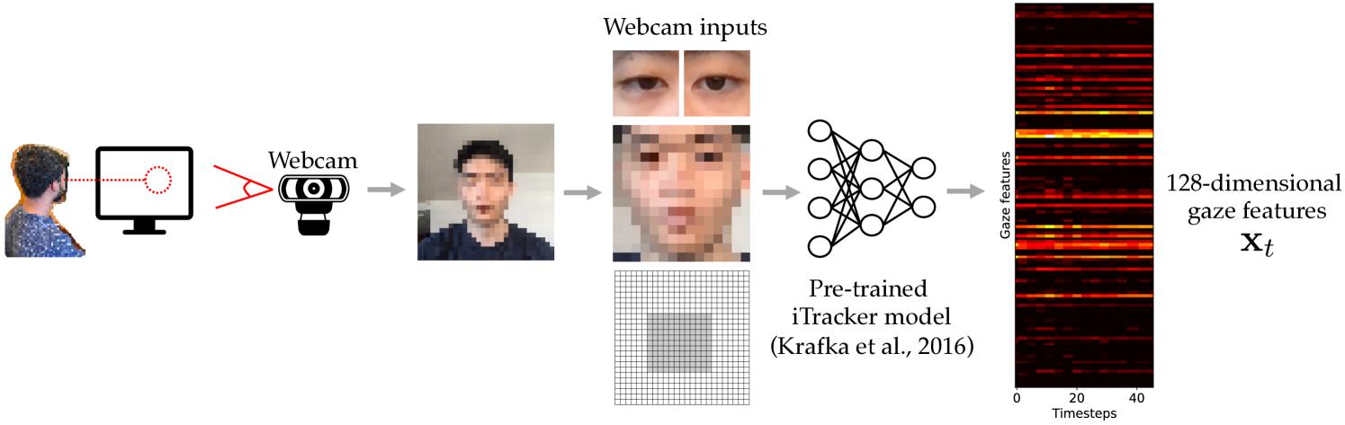
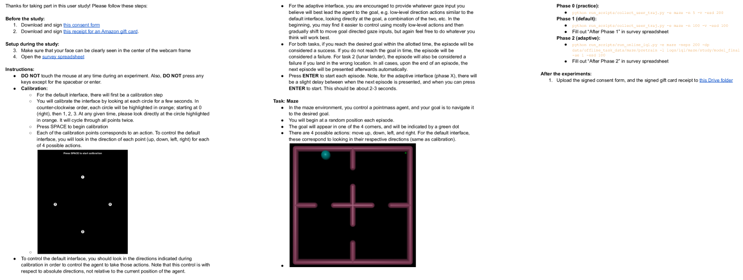
Our experiments focus on evaluating ORBIT’s ability to learn an effective interface through a combination of offline pre-training and online fine-tuning. To do so, we conduct a user study with 12 participants who use their eye gaze to modulate a noisy command signal from their webcam (see Fig. 3) to perform the simulated 2D continuous navigation task from [51] (illustration in Fig. 5a). The state is the current 2D position, the user’s command is a 128-dimensional signal from their webcam, and the action is a 2D velocity. The eye gaze signals are the same used in prior work on RL-based adaptive interfaces [6, 7], and consist of representations from iTracker [52].
While iTracker is no longer the state of the art in gaze tracking, our goal here is not to develop the best possible gaze control interface, but to study if RL can be used to learn a better control interface that operates on noisy command signals. We also note that while this 2D navigation task is relatively simple, it represents a more challenging control task than those in prior work that use this command signal, which are limited to either contextual bandits, or settings where individual command signals are never mapped directly to low-level actions.
Baseline: directional interface. The ‘default’ interface enables the user to move left/right/up/down by looking at the left/right/top/bottom half of the screen. We calibrate this interface once at the start of each study by asking the user to look at the left, right, top, and bottom portions of the screen one by one, recording 20 webcam images for each location, and training a 2D gaze position estimator conditioned on iTracker command signals, as done in the original work [52]. In our setting, this calibrated interface is a strong baseline, since it assumes access to commands and ground-truth action labels for supervised calibration, whereas our ORBIT method does not assume access to paired data. While this interface may not be optimal for this task, we aim not to design the best possible baseline interface, but to investigate whether ORBIT can be used to improve upon the interface used to collect its training data.
Experiment design. Each of the 12 participants completed two phases of experiments. In phase A, they use the default, directional interface for 100 episodes. Note that the directional interface is non-adaptive, so it cannot improve with additional evaluation. In phase B, they operate an adaptive interface that is initially pre-trained on the offline data then fine-tuned online by ORBIT for 200 episodes. Each episode takes approximately 18 seconds on average. To avoid the confounding effect of user improvement or fatigue, we counterbalance the order of phases A and B. Users are informed of how each interface operates before each phase.
Cold start problem. New users can face the “cold start problem” of not having past data for training their interface. We also face this challenge in our experiments, since collecting a large offline dataset before running an online fine-tuning experiment is difficult to accomplish within the maximum duration of a user study for a given participant. Hence, we collect a large offline dataset of 1200 episodes of an expert user (the first author) performing tasks using their eye gaze and the default directional interface. We use this dataset to pre-train an interface for each of the 12 participants.
IV-A Can we learn an effective interface through RL?
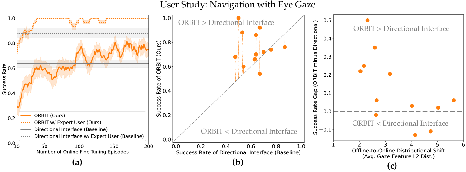
Offline pre-training enables efficient online fine-tuning. The results in Fig. 4a show that, through offline pre-training and online fine-tuning, ORBIT (orange) learns an interface that better enables users to navigate than the default, directional interface (gray). For the 12 participants, ORBIT (solid orange) outperforms the directional interface (solid gray) after 100 episodes, or 30 minutes, of online fine-tuning. In contrast, without any offline pre-training, we find that purely online RL from sparse rewards is not capable of learning an effective interface at all, even when we simulate idealized user commands (see the ablation experiment for Q10 in Sec. V). These results show that offline pre-training is essential for making online fine-tuning from sparse rewards feasible and efficient.
ORBIT performance improves under distributional shift in command signals between the offline and online data. If we evaluate ORBIT on the same expert user who generated the offline data (dashed curves in Fig. 4a), we find that it takes less than 20 episodes of online fine-tuning before ORBIT (dashed orange) starts to outperform the directional interface (dashed gray), and that ORBIT converges to a 100% success rate. Furthermore, Fig. 4c shows that participants whose command signals are closer to the offline data distribution perform better with ORBIT. These results suggest that ORBIT works best when the user who is operating the interface during online fine-tuning is similar to the user that generated the offline data.
While data personalization poses a potential challenge here with the discrepancy between the user who generates the offline data and the user who operates the interface, we find that offline pre-training on one user’s data can still provide a good initialization for a different user, as evidenced by fine-tuning quickly developing an effective interface (solid orange in Fig. 4a). In spite of the data personalization challenge in our evaluation, ORBIT still outperforms the default interface after fine-tuning. This suggests that ORBIT can be deployed to new users in practice by leveraging data from past users. We hypothesize that with greater data diversity from multiple users, data personalization is less likely to be problematic.
ORBIT is most helpful for users who struggle with their existing interface. While Fig. 4a shows average performance across the 12 participants, the scatter plot in Fig. 4b breaks down the performance of ORBIT (y-axis) vs. the directional interface (x-axis) for each participant. We find that ORBIT tends to perform better for users who perform worse with the directional interface, and that users who can already use the directional interface well can see a small drop in performance. These results suggest that ORBIT would be more helpful for users who struggle to use their existing interface.
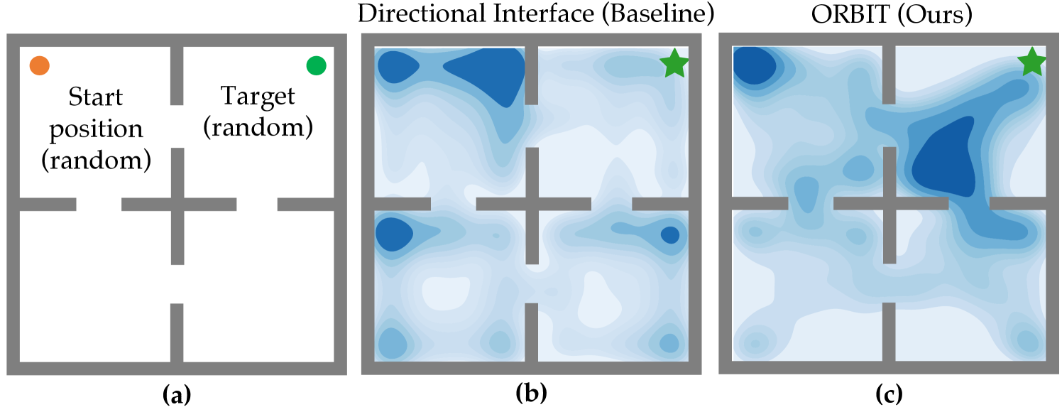
Emergence of shared autonomy. Fig. 5b and 5c illustrate the positions that users occupy when navigating to the green star in the top-right corner. With the directional interface, users tend to get stuck in corners of the other rooms. With ORBIT, users spend less time in the wrong rooms, and only tend to get stuck briefly at corners or bottlenecks near the target. These figures illustrate a key advantage of ORBIT: because the interface is trained through RL, it more often takes actions that have a chance of performing a task, while avoiding actions that are unlikely to do so. For example, users tend to have trouble passing through the narrow corridors separating the rooms using the directional interface, since this requires precise gaze commands. With ORBIT, the interface gets stuck less often, even with noisy gaze commands. This “shared autonomy” emerges naturally through RL, without being explicitly incorporated into the interface.
V Ablations and Showcases in Different Domains
To perform ablations of ORBIT at a scale that would be impractical for a user study, we simulate noisy, high-dimensional user commands for the navigation task by randomly projecting the optimal 2D velocity into a 128-dimensional space of command signals, and adding i.i.d. Gaussian noise () to the intended velocity at each timestep. Also, similarly as in [3], we repeat the previous command with probability 0.75 (i.e., lagging).
We aim to answer the following. Q1: Is offline RL beneficial in our setting, or can we simply use behavior cloning (BC)? Q2: What if we only run BC on successful trajectories? Q3: Can we directly apply vanilla IQL by simply concatenating command signals with environment states, as done in [3]? Q4: What is the effect of regularizing the trajectory encoder with negative data augmentation? Q5: What is the effect of regularizing the encoders with an information bottleneck? Q6: What is the effect of training a separate history encoder for the policy, compared to reusing the trajectory encoder? Q7: What is the effect of conditioning the value functions on an embedding of the full trajectory vs. a partial trajectory? Q8: What is the effect of training the trajectory encoder on reward prediction, instead of end-to-end training on the IQL losses and ? Q9: What is the effect of the offline dataset size? Q10: What if we do not have offline data, and have to acquire an interface purely through online RL?
To answer Q1-9, we train offline on 1K trajectories with no fine-tuning. To answer Q10, we run online RL for 500 episodes with no offline pre-training. We note that our baseline for Q3, where we concatenate environment states with command signals as the RL observation space, and then run offline RL directly, is to our knowledge the only type of RL baseline that can be applied to this setting. Other prior RL methods would require additional assumptions, such as a task-agnostic reward function, the user’s task distribution, or a prior interface [3, 6, 7]. In fact, this baseline can be viewed as an offline version of [3] without the components that would require additional assumptions. The results in Table I show that ORBIT outperforms all of its ablated variants and the baselines.
Success Rate Episode Length Directional Interface (Baseline) Behavior Cloning (Baseline) (Q1) Filtered Behavior Cloning (Baseline) (Q2) Vanilla IQL (Baseline based on [3]) (Q3) ORBIT (Ours) ORBIT w/o NDA (Q4) ORBIT w/o VIB (Q5) ORBIT w/o Separate History Encoder (Q6) ORBIT w/ Partial Trajectory Embedding (Q7) ORBIT w/ End-to-End Trajectory Encoder (Q8) ORBIT w/ 500 Offline Trajectories (Q9) ORBIT w/ 100 Offline Trajectories (Q9) ORBIT w/o Offline Pre-Training (Q10)
![[Uncaptioned image]](https://cdn.awesomepapers.org/papers/38416d17-93ec-40e8-8fc5-f5edafb64a7d/lunarlander_square.jpg)
![[Uncaptioned image]](https://cdn.awesomepapers.org/papers/38416d17-93ec-40e8-8fc5-f5edafb64a7d/sawyer_pusher.png) (Simulated Commands)
(Webcam Commands)
Success Rate
Success Rate
Directional
ORBIT
(Simulated Commands)
(Webcam Commands)
Success Rate
Success Rate
Directional
ORBIT
To showcase ORBIT in other domains, we evaluate ORBIT on the Lunar Lander and Sawyer Pushing tasks from [51] (images in Table II). For Sawyer Pushing, we have an expert user (the first author) provide real webcam command signals. For Lunar Lander, we simulate noisy, high-dimensional user commands as in the ablations. The results in Table II show that ORBIT outperforms the default interface in both domains.
VI Discussion
Through a user study with 12 participants, we show that offline RL can be used to bootstrap the online fine-tuning of an assistive human-machine interface that enables people to perform a simulated navigation task by using their eye gaze to modulate a noisy, 128-dimensional command signal from their webcam. Large-scale ablation experiments with simulated user commands show that, while our method has many moving parts, each is well-motivated and enables the user to succeed at their desired tasks more frequently.
Our experiments are limited to relatively simple tasks in simulated domains. Scaling an offline RL method such as ORBIT to more practical and challenging real-world applications may require larger and more diverse datasets. This could be achieved through more widespread use of assistive control systems, such that users are constantly collecting data while performing daily activities, and data may be shared across users.
ORBIT is limited by its inability to learn from data collected in the environment without the user in the loop. In real-world applications such as assistive robotics, the robot can interact with the environment in an unsupervised manner without the user present, e.g., in order to explore the state space or learn the environment dynamics. A promising direction for future work would be to integrate data that is collected autonomously into the ORBIT pipeline, using an algorithm like COG [53]. Another promising idea is to use offline meta-RL [54, 55, 56] to learn from heterogeneous offline data collected from multiple users, or from the same user at different times.
VII Acknowledgements
Thanks to members of the InterACT and RAIL labs at UC Berkeley for feedback on this project, especially Sean Chen. This work was supported by ARL DCIST CRA W911NF-17-2-0181, ARO W911NF-21-1-0097, Weill Neurohub, Semiconductor Research Corporation, and CIFAR.
References
- [1] Patrick M Pilarski, Michael R Dawson, Thomas Degris, Farbod Fahimi, Jason P Carey, and Richard S Sutton. Online human training of a myoelectric prosthesis controller via actor-critic reinforcement learning. In IEEE International Conference on Rehabilitation Robotics, 2011.
- [2] Alexander Broad, Todd David Murphey, and Brenna Dee Argall. Learning models for shared control of human-machine systems with unknown dynamics. In Robotics: Science and Systems, 2017.
- [3] Siddharth Reddy, Anca D Dragan, and Sergey Levine. Shared autonomy via deep reinforcement learning. arXiv preprint arXiv:1802.01744, 2018.
- [4] Charles Schaff and Matthew R Walter. Residual policy learning for shared autonomy. arXiv preprint arXiv:2004.05097, 2020.
- [5] Yuqing Du, Stas Tiomkin, Emre Kiciman, Daniel Polani, Pieter Abbeel, and Anca Dragan. AvE: Assistance via empowerment. arXiv preprint arXiv:2006.14796, 2020.
- [6] Jensen Gao, Siddharth Reddy, Glen Berseth, Nicholas Hardy, Nikhilesh Natraj, Karunesh Ganguly, Anca Dragan, and Sergey Levine. X2T: Training an x-to-text typing interface with online learning from user feedback. In International Conference on Learning Representations, 2021.
- [7] Sean Chen, Jensen Gao, Siddharth Reddy, Glen Berseth, Anca D. Dragan, and Sergey Levine. ASHA: Assistive teleoperation via human-in-the-loop reinforcement learning. arXiv preprint arXiv:2202.02465, 2022.
- [8] Scott Fujimoto, David Meger, and Doina Precup. Off-policy deep reinforcement learning without exploration. In International Conference on Machine Learning, 2019.
- [9] Yifan Wu, George Tucker, and Ofir Nachum. Behavior regularized offline reinforcement learning. arXiv preprint arXiv:1911.11361, 2019.
- [10] Aviral Kumar, Aurick Zhou, George Tucker, and Sergey Levine. Conservative Q-learning for offline reinforcement learning. Neural Information Processing Systems, 2020.
- [11] Tianhe Yu, Garrett Thomas, Lantao Yu, Stefano Ermon, James Y Zou, Sergey Levine, Chelsea Finn, and Tengyu Ma. MOPO: Model-based offline policy optimization. Neural Information Processing Systems, 2020.
- [12] Rahul Kidambi, Aravind Rajeswaran, Praneeth Netrapalli, and Thorsten Joachims. MOReL: Model-based offline reinforcement learning. Neural Information Processing Systems, 2020.
- [13] Ashvin Nair, Abhishek Gupta, Murtaza Dalal, and Sergey Levine. AWAC: Accelerating online reinforcement learning with offline datasets. arXiv preprint arXiv:2006.09359, 2020.
- [14] Jian Shen, Mingcheng Chen, Zhicheng Zhang, Zhengyu Yang, Weinan Zhang, and Yong Yu. Model-based offline policy optimization with distribution correcting regularization. In European Conference on Machine Learning and Knowledge Discovery in Databases, 2021.
- [15] Scott Emmons, Benjamin Eysenbach, Ilya Kostrikov, and Sergey Levine. RvS: What is essential for offline RL via supervised learning? arXiv preprint arXiv:2112.10751, 2021.
- [16] Ilya Kostrikov, Ashvin Nair, and Sergey Levine. Offline reinforcement learning with implicit Q-learning. arXiv preprint arXiv:2110.06169, 2021.
- [17] Assaf Hallak, Dotan Di Castro, and Shie Mannor. Contextual Markov decision processes. arXiv preprint arXiv:1502.02259, 2015.
- [18] Luisa Zintgraf, Kyriacos Shiarlis, Maximilian Igl, Sebastian Schulze, Yarin Gal, Katja Hofmann, and Shimon Whiteson. VariBAD: A very good method for Bayes-adaptive deep RL via meta-learning. arXiv preprint arXiv:1910.08348, 2019.
- [19] Alexander A Alemi, Ian Fischer, Joshua V Dillon, and Kevin Murphy. Deep variational information bottleneck. arXiv preprint arXiv:1612.00410, 2016.
- [20] Alessandro Achille and Stefano Soatto. Information dropout: Learning optimal representations through noisy computation. IEEE Transactions on Pattern Analysis and Machine Intelligence, 2018.
- [21] Kyunghyun Cho, Bart Van Merriënboer, Dzmitry Bahdanau, and Yoshua Bengio. On the properties of neural machine translation: Encoder-decoder approaches. arXiv preprint arXiv:1409.1259, 2014.
- [22] Xue Bin Peng, Aviral Kumar, Grace Zhang, and Sergey Levine. Advantage-weighted regression: Simple and scalable off-policy reinforcement learning. arXiv preprint arXiv:1910.00177, 2019.
- [23] Kate Rakelly, Aurick Zhou, Chelsea Finn, Sergey Levine, and Deirdre Quillen. Efficient off-policy meta-reinforcement learning via probabilistic context variables. In International Conference on Machine Learning, 2019.
- [24] Vikash Gilja, Paul Nuyujukian, Cindy A Chestek, John P Cunningham, M Yu Byron, Joline M Fan, Mark M Churchland, Matthew T Kaufman, Jonathan C Kao, Stephen I Ryu, et al. A high-performance neural prosthesis enabled by control algorithm design. Nature neuroscience, 2012.
- [25] Siddharth Dangi, Amy L Orsborn, Helene G Moorman, and Jose M Carmena. Design and analysis of closed-loop decoder adaptation algorithms for brain-machine interfaces. Neural computation, 2013.
- [26] Siddharth Dangi, Suraj Gowda, Helene G Moorman, Amy L Orsborn, Kelvin So, Maryam Shanechi, and Jose M Carmena. Continuous closed-loop decoder adaptation with a recursive maximum likelihood algorithm allows for rapid performance acquisition in brain-machine interfaces. Neural computation, 2014.
- [27] Josh Merel, David Carlson, Liam Paninski, and John P Cunningham. Neuroprosthetic decoder training as imitation learning. arXiv preprint arXiv:1511.04156, 2015.
- [28] Gopala K Anumanchipalli, Josh Chartier, and Edward F Chang. Speech synthesis from neural decoding of spoken sentences. Nature, 2019.
- [29] Francis R Willett, Donald T Avansino, Leigh R Hochberg, Jaimie M Henderson, and Krishna V Shenoy. High-performance brain-to-text communication via imagined handwriting. bioRxiv, 2020.
- [30] Sida I Wang, Percy Liang, and Christopher D Manning. Learning language games through interaction. arXiv preprint arXiv:1606.02447, 2016.
- [31] Siddharth Karamcheti, Dorsa Sadigh, and Percy Liang. Learning adaptive language interfaces through decomposition. arXiv preprint arXiv:2010.05190, 2020.
- [32] Michael Ahn, Anthony Brohan, Noah Brown, Yevgen Chebotar, Omar Cortes, Byron David, Chelsea Finn, Keerthana Gopalakrishnan, Karol Hausman, Alex Herzog, et al. Do as I can, not as I say: Grounding language in robotic affordances. arXiv preprint arXiv:2204.01691, 2022.
- [33] Sidney S Fels and Geoffrey E Hinton. Glove-Talk: A neural network interface between a data-glove and a speech synthesizer. IEEE Transactions on Neural Networks, 1993.
- [34] Sidney S Fels and Geoffrey E Hinton. Glove-Talk II—a neural-network interface which maps gestures to parallel formant speech synthesizer controls. IEEE Transactions on Neural Networks, 1997.
- [35] Andy Hunt and Marcelo M Wanderley. Mapping performer parameters to synthesis engines. Organised Sound, 2002.
- [36] Hyun K Kim, J Biggs, W Schloerb, M Carmena, Mikhail A Lebedev, Miguel AL Nicolelis, and Mandayam A Srinivasan. Continuous shared control for stabilizing reaching and grasping with brain-machine interfaces. IEEE Transactions on Biomedical Engineering, 2006.
- [37] David P McMullen, Guy Hotson, Kapil D Katyal, Brock A Wester, Matthew S Fifer, Timothy G McGee, Andrew Harris, Matthew S Johannes, R Jacob Vogelstein, Alan D Ravitz, et al. Demonstration of a semi-autonomous hybrid brain–machine interface using human intracranial EEG, eye tracking, and computer vision to control a robotic upper limb prosthetic. IEEE Transactions on Neural Systems and Rehabilitation Engineering, 2013.
- [38] Tom Carlson and Yiannis Demiris. Collaborative control for a robotic wheelchair: evaluation of performance, attention, and workload. IEEE Transactions on Systems, Man, and Cybernetics, 2012.
- [39] Brenna D Argall. Modular and adaptive wheelchair automation. In Experimental Robotics, 2016.
- [40] Shervin Javdani. Acting under Uncertainty for Information Gathering and Shared Autonomy. PhD thesis, Carnegie Mellon University, 2017.
- [41] Hong Jun Jeon, Dylan P Losey, and Dorsa Sadigh. Shared autonomy with learned latent actions. arXiv preprint arXiv:2005.03210, 2020.
- [42] James MacGlashan, Mark K Ho, Robert Loftin, Bei Peng, David Roberts, Matthew E Taylor, and Michael L Littman. Interactive learning from policy-dependent human feedback. arXiv preprint arXiv:1701.06049, 2017.
- [43] Dilip Arumugam, Jun Ki Lee, Sophie Saskin, and Michael L Littman. Deep reinforcement learning from policy-dependent human feedback. arXiv preprint arXiv:1902.04257, 2019.
- [44] W Bradley Knox and Peter Stone. Interactively shaping agents via human reinforcement: The TAMER framework. In International Conference on Knowledge Capture, 2009.
- [45] Garrett Warnell, Nicholas Waytowich, Vernon Lawhern, and Peter Stone. Deep TAMER: Interactive agent shaping in high-dimensional state spaces. arXiv preprint arXiv:1709.10163, 2017.
- [46] Dorsa Sadigh, Anca D Dragan, Shankar Sastry, and Sanjit A Seshia. Active preference-based learning of reward functions. In Robotics: Science and Systems, 2017.
- [47] Paul F Christiano, Jan Leike, Tom Brown, Miljan Martic, Shane Legg, and Dario Amodei. Deep reinforcement learning from human preferences. In Neural Information Processing Systems, 2017.
- [48] Borja Ibarz, Jan Leike, Tobias Pohlen, Geoffrey Irving, Shane Legg, and Dario Amodei. Reward learning from human preferences and demonstrations in Atari. Neural Information Processing Systems, 2018.
- [49] Nisan Stiennon, Long Ouyang, Jeffrey Wu, Daniel Ziegler, Ryan Lowe, Chelsea Voss, Alec Radford, Dario Amodei, and Paul F Christiano. Learning to summarize with human feedback. Neural Information Processing Systems, 2020.
- [50] Erdem Bıyık, Dylan P Losey, Malayandi Palan, Nicholas C Landolfi, Gleb Shevchuk, and Dorsa Sadigh. Learning reward functions from diverse sources of human feedback: Optimally integrating demonstrations and preferences. International Journal of Robotics Research, 2021.
- [51] Dibya Ghosh, Abhishek Gupta, Ashwin Reddy, Justin Fu, Coline Devin, Benjamin Eysenbach, and Sergey Levine. Learning to reach goals via iterated supervised learning. arXiv preprint arXiv:1912.06088, 2019.
- [52] Kyle Krafka, Aditya Khosla, Petr Kellnhofer, Harini Kannan, Suchendra Bhandarkar, Wojciech Matusik, and Antonio Torralba. Eye tracking for everyone. In IEEE Conference on Computer Vision and Pattern Recognition, 2016.
- [53] Avi Singh, Albert Yu, Jonathan Yang, Jesse Zhang, Aviral Kumar, and Sergey Levine. COG: Connecting new skills to past experience with offline reinforcement learning. arXiv preprint arXiv:2010.14500, 2020.
- [54] Vitchyr H Pong, Ashvin Nair, Laura Smith, Catherine Huang, and Sergey Levine. Offline meta-reinforcement learning with online self-supervision. arXiv preprint arXiv:2107.03974, 2021.
- [55] Tony Z Zhao, Jianlan Luo, Oleg Sushkov, Rugile Pevceviciute, Nicolas Heess, Jon Scholz, Stefan Schaal, and Sergey Levine. Offline meta-reinforcement learning for industrial insertion. arXiv preprint arXiv:2110.04276, 2021.
- [56] Eric Mitchell, Rafael Rafailov, Xue Bin Peng, Sergey Levine, and Chelsea Finn. Offline meta-reinforcement learning with advantage weighting. In International Conference on Machine Learning, 2021.
- [57] Diederik P Kingma and Jimmy Ba. Adam: A method for stochastic optimization. arXiv preprint arXiv:1412.6980, 2014.
- [58] John Schulman, Filip Wolski, Prafulla Dhariwal, Alec Radford, and Oleg Klimov. Proximal policy optimization algorithms. arXiv preprint arXiv:1707.06347, 2017.
- [59] Antonin Raffin, Ashley Hill, Adam Gleave, Anssi Kanervisto, Maximilian Ernestus, and Noah Dormann. Stable-Baselines3: Reliable reinforcement learning implementations. Journal of Machine Learning Research, 2021.
Appendix A Appendix
A-A History Encoder Architecture
When choosing an architecture for the history encoder , we initially tried the same recurrent architecture as the trajectory encoder from Sec. II-A, but found that this tended to overfit to the sequences of states in the offline data—see the ablation experiment for Q6 in Sec. V. To address this issue, we model the history encoder as a product of independent Gaussian factors, similar to the inference network architecture used by [23]. This results in a Gaussian posterior,
| (8) |
This architecture requires fewer parameters than an equivalent recurrent architecture, but is invariant to the order of the timesteps.
A-B Implementation
For the navigation task, we pre-train the trajectory encoder and history encoder with 50K gradient steps, the value functions and with 200K steps, and the policy with 200K steps. For the pushing task, we pre-train the encoders with 100K gradient steps, and the value functions with 300K steps. We set in Equation 4 for the navigation task, for the pushing task, and for the Lunar Lander game. We set in Equation 6 for the navigation task in the user study, for the pushing task, and for the navigation task in the ablation experiments as well as the Lunar Lander game simulations. In IQL, we set the expectile . We set in Equation 5 in the navigation task, for the pushing task, and in the Lunar Lander game. We set the dimensionality of the latent space to in the navigation task, for the pushing task, and in the Lunar Lander game. To optimize all of our losses, we use the Adam optimizer [57] with an initial learning rate of . Following the IQL method, we use a constant learning rate for training the value functions, and cosine scheduling for training the encoders and policy. We use a batch size of 16 sequences to train the trajectory encoder, and batch size of 256 to train the value functions and policy. We set the soft -function update . We set in line 10 of Alg. 1.
The trajectory encoder architecture maps 64-dimensional linear layer ReLU (previous representation, ) 64-dimensional GRU linear layer means and standard deviations of latent features. For the pushing task and the Lunar Lander game, we apply a dropout rate of 0.5 to the output of the first ReLU layer, and increase the number of hidden units in the GRU layer from 64 to 512. The reward decoder architecture is a feedforward network with 2 layers of 32 hidden units each and ReLU activations. The history encoder architecture is the same, but with 64 hidden units, and a sliding window of the past 30 timesteps in the navigation task, the past 50 timesteps in the pushing task, and the past 200 timesteps (i.e., the full history) in the Lunar Lander game. For the pushing task and the Lunar Lander game, we increase the number of hidden units in the second hidden layer from 64 to 512. The -function and value function architectures are both feedforward networks with 2 layers of 64 hidden units each and ReLU activations, and a dropout rate of 0.01. The policy architecture is a feedforward network with 2 layers of 64 hidden units each and ReLU activations, with a dropout rate of 0.1. For the pushing task and the Lunar Lander game, we increase the number of hidden units in both hidden layers of the -function, value function, and policy architectures from 64 to 256.
For the navigation task, for each gradient step on the trajectory encoder loss in Equation 4, we compute the loss terms and as follows. We sample a batch of trajectories, compute the mean of the loss terms associated with positive rewards in the binary cross-entropy loss , and compute the mean of the loss terms associated with negative rewards. We then compute the negative data augmentation loss for the batch by randomly permuting the alignment between embeddings and state sequences, and taking the mean of the loss terms. We then weigh the three mean loss terms—positive rewards, negative rewards, and negative data augmentation—equally when taking a gradient step. For the Lunar Lander and pushing tasks, we take a slightly different approach to weighting these terms. The positive rewards have a weight of , negative rewards a weight of , negative data augmentation a weight of , and negative data augmentation for transitions with a reward of before permutation.
For all offline pre-training and simulation experiments, we trained and ran our models on an RTX 2080 GPU. We performed the user studies on one consumer-grade desktop computer with a Logitech C920x webcam.
Where applicable, and if not otherwise specified, our implementation of baseline methods and ablations of ORBIT use the same hyperparameter values as our implementation of the full ORBIT algorithm.
A-C Simulation Experiments
When simulating noisy user commands, we add Gaussian noise with standard deviation in the navigation task, and in the Lunar Lander game. We repeat the user’s previous command (i.e., lag) with probability in the navigation task, and in the Lunar Lander game. To follow the real eye gaze capture pipeline from the user study as closely as possible, we apply a random linear projection to the simulated user’s noisy 2D velocity that transforms this 2D intent into a 128-dimensional command signal, then clamp the projected signal using the ReLU function. When calibrating the default directional interface, we only collect 10 samples per direction (in contrast to the 20 samples used in the user study). The offline data consists of 100 episodes per default interface—10 different default interfaces (each trained with a different random seed) in the navigation task, and 50 different default interfaces in the Lunar Lander game—yielding a total of 1K episodes (98253 timesteps) in the navigation task, and 5K episodes (474984 timesteps) in the Lunar Lander game.
We train an agent to act as the simulated user using the proximal policy optimization algorithm (PPO) [58] and the default hyperparameter values from the Stable Baselines3 library [59]. We take 2048 environment steps per gradient step in the navigation task, and 8192 environment steps per gradient step in the Lunar Lander game. We set the entropy coefficient to 0.01. The policy architecture is a feedforward network with 2 layers of 32 hidden units each and ReLU activations. We run PPO for 3 million timesteps in the navigation task, and 1M timesteps in the Lunar Lander game. We sample actions from the policy, instead of executing the action with the highest likelihood according to the policy.
For the ablation experiment addressing Q8, we set in Equation 4.
For the ablation experiment addressing Q10, we run online RL from scratch with no offline pre-training. Unlike the online fine-tuning procedure described in Section II-C, for this experiment we use negative data augmentation and do not freeze the reward decoder. We take the same number of gradient steps per episode as the number of environment steps in the previous episode. We set in line 10 of Alg. 1.
For the Lunar Lander simulation experiments, we collect an offline dataset by calibrating 20 different default interfaces and collecting 100 episodes using each of them, yielding a total of 2K episodes total in the offline dataset.
A-D Sawyer Pushing Experiments with Real Webcam Commands
We found that online fine-tuning did not substantially improve performance, so Table II shows the results for purely-offline RL (i.e., no online fine-tuning). We collect the offline dataset by calibrating 12 different default interfaces and collecting 100 episodes using each of them, yielding a total of 1200 episodes (180561 timesteps).
In our initial experiments with the pushing task, we found that the trajectory encoder learned to generate latent embeddings that, instead of representing the user’s intent, represent whether or not the states in the trajectory are associated with high or low reward—this leads to the formation of two separate clusters of latents for successes and failures, instead of separate clusters for different goals or tasks. To address this issue, we train a discriminator to classify whether a latent embedding belongs to a successful trajectory or failed trajectory. We class-balance this binary classification loss to contain equal proportions of positive and negative examples. We then add the following term to the trajectory encoder training loss in Equation 4: the log-likelihood of the discriminator classifying latents from failed trajectories as successful. This additional term encourages the distribution of latent embeddings of successful trajectories to match the distribution of latents for failed trajectories. We alternate between taking 1 gradient step on the binary classification loss to update the discriminator, and taking 1 gradient step on Equation 4. We weight both loss terms with a coefficient of . We model the discriminator as a feedforward network with 2 hidden layers of 32 units each and ReLU activations. To determine whether the discriminator loss could be useful for a particular domain, we recommend visualizing the latent embeddings of the user’s intent—if there are two distinct clusters corresponding to successes and failures, then the discriminator loss could improve intent inference.
A-E Environments
In the pushing task, there are 4 possible 2D goal positions for the puck, each in the corner of a rectangle. At the beginning of each episode, the puck and end effector are both reset to the center of this rectangle. There are 8 discrete actions, corresponding to unit velocities in the 4 cardinal directions and 4 diagonal directions. The 4D state consists of the 2D end effector position and 2D puck position. The state and goal positions are normalized to the range .
In the Lunar Lander game, we flatten the terrain, partition the terrain into 5 equally-sized landing zones, and choose one uniformly at random at the beginning of each episode to be the simulated user’s desired landing zone. To make the game easier, we set the initial force perturbation on the lander to zero.
The maximum episode length in the navigation task, pushing task, and the Lunar Lander game is 200 timesteps.
Sparse rewards are set to and in the navigation and pushing tasks (to encourage faster task completion), and and in the Lunar Lander game (since episode length does not matter). The value functions in the Lunar Lander game have a sigmoid output activation layer, since the values are bounded between and .
A-F User Study
| Directional Interface | ORBIT | ||
|---|---|---|---|
| The system performed the task I wanted | 4.42 | 4.75 | |
| I felt in control | 4.50 | 4.17 | |
| The system responded to my input in the way that I expected | 4.33 | 3.67 | |
| The system was competent at performing tasks… | |||
| …even if they weren’t the tasks I wanted | 3.92 | 4.83 | |
| The system improved over time | 2.50 | 6.17 | |
| I improved at using the system over time | 4.92 | 5.50 | |
| I always looked directly at my final target… | |||
| …holding the same gaze throughout an episode | 1.75 | 2.75 | |
| I compensated for flaws in the system… | |||
| …by changing my gaze over time… | |||
| …, e.g., by exaggerating looking in certain directions | 5.00 | 5.55 |
We recruited 9 male and 3 female participants, with an average age of 22. We obtained informed consent from each participant, as well as IRB approval for our study. Each participant was provided with the rules of the task (see Fig. 6), and compensated with a $20 Amazon gift card.
Given that the reward for the navigation task is very simple for a person to compute (+1 for reaching the goal, 0 otherwise), we automate the reward signal instead of asking the user for a button press. In a similar user study from prior work [6], it has been shown that automated sparse rewards match user-provided rewards 98.6% of the time.
All participants used the same webcam setup and the same desktop computer in the same room. The offline data was collected from the expert user (the first author) in 12 sessions of 100 episodes (94100 steps total), with a new default directional interface calibrated at the beginning of each session to account for changes in the webcam image distribution (e.g., background lighting). During the online fine-tuning phase, we take and gradient steps in lines 8 and 12 in Alg. 1. We use the Adam optimizer with the same hyperparameter settings as in the offline pre-training phase (i.e., a constant learning rate of ).
The only personal data logged during the user studies were 128-dimensional eye gaze features, which cannot be used to uniquely recover the original face or eye images from the webcam.
When prompted to “please describe your command strategy”, participants responded as follows.
User 5:
After Phase A:
Feel like it’s much more difficult to go left-right than top-down. Probably because the face shifts more in the horizontal direction. So every time I feel that it is very very difficult say to go right, I’ll shift face leftwards and it becomes easier, vice versa.
After Phase B:
Look at final target if in same quadrant, otherwise look at some waypoints
User 6:
After Phase A:
I generally tried to look to the edge of the screen, but would sometimes follow the dot in different directions.
After Phase B:
First I would look at the target, and if the ball got stuck, I would look at the exaggerated direction of the target, or use basic left/right/up/down directions.
User 7:
After Phase A:
I’d move my eyes in the direction I wanted the ball to move
User 8:
After Phase A:
To get through door: first get on wall of door. Then gaze in one direction and quickly switch gaze direction to try to get through door. Repeat until through door If in same room as target: first gaze in one direction to get on on wall such that i am strraight line away from target. Then move to direct by gazing in one direction
After Phase B:
Look at either center of rooms or the target location if already in same room as target location. Do exaggerated eye motions to get unstuck if stuck on a wall.
User 11:
After Phase A:
At first I looked at the points shown during calibration, but later I found there were particular points on the screen which more reliably mapped to the direction I wanted (even if they weren’t exactly the calibration points), so I looekd at those.
After Phase B:
Look at either the goal or the nearest doorway between rooms. If the agent isn’t responding, alternate strategies.
User 12:
After Phase A:
Mostly looking directly at the direction I wanted the agent to move in at a finer-grained level
After Phase B:
I looked directly at the goal initially, but if that didn’t work or the agent got stuck, then I would look in the direction I wanted the agent to move in (up/down/left/right) at a lower level
The heatmaps in Fig. 5 are generated by filtering out state transitions where consecutives states are identical to each other (i.e., repeated). For ORBIT, we only visualize the last 50 episodes of fine-tuning.