This paper was converted on www.awesomepapers.org from LaTeX by an anonymous user.
Want to know more? Visit the Converter page.

Bootstraps for Dynamic Panel Threshold Models

Woosik Gong University of Wisconsin-Madison. Email: wgong28@wisc.edu. This research was supported by the BK21 FOUR (Fostering Outstanding Universities for Research) funded by the Ministry of Education(MOE, Korea) and National Research Foundation of Korea(NRF). The author is also grateful to the student travel grant award by the IAAE 2022 conference.    Myung Hwan Seo Seoul National University. Email: myunghseo@snu.ac.kr. This work was supported by the Ministry of Education of the Republic of Korea and the National Research Foundation of Korea (NRF-2018S1A5A2A01033487)
Abstract

This paper develops valid bootstrap inference methods for the dynamic short panel threshold regression. We demonstrate that the standard nonparametric bootstrap is inconsistent for the first-differenced generalized method of moments (GMM) estimator. The inconsistency arises from an n1/4n^{1/4}-consistent non-normal asymptotic distribution of the threshold estimator when the true parameter lies in the continuity region of the parameter space, which stems from the rank deficiency of the approximate Jacobian of the sample moment conditions on the continuity region. To address this, we propose a grid bootstrap to construct confidence intervals for the threshold and a residual bootstrap to construct confidence intervals for the coefficients. They are shown to be valid regardless of the model’s continuity. Moreover, we establish a uniform validity for the grid bootstrap. A set of Monte Carlo experiments demonstrates that the proposed bootstraps improve upon the standard nonparametric bootstrap. An empirical application to a firm investment model illustrates our methods.

KEYWORDS: Dynamic Panel Threshold; Kink; Bootstrap; Endogeneity; Identification; Rank Deficiency; Uniformity.

JEL: C12, C23, C24

1 Introduction

Threshold regression models have been widely used by empirical researchers, which have been more fruitful because of their extensions to the panel data context. Estimation and inference methods for the threshold model in non-dynamic panels were developed by Hansen, 1999b and Wang, (2015). Dynamic panel threshold models were considered by Seo and Shin, (2016), which proposes the generalized method of moments (GMM) estimation by generalizing the Arellano and Bond, (1991) dynamic panel estimator. A latent group structure in the parameters of the panel threshold model was investigated by Miao et al., 2020b .

Applications of the panel threshold models cover numerous topics in economics. The effect of debt on economic growth is a well-known example that has been analyzed using the panel threshold models, e.g., Adam and Bevan, (2005), Cecchetti et al., (2011) and Chudik et al., (2017). Another example is the threshold effect of inflation on economic growth such as the works by Khan and Senhadji, (2001), Rousseau and Wachtel, (2002), Bick, (2010), and Kremer et al., (2013). The benefit of foreign direct investment to productivity growth that depends on the regime determined by absorptive capacity is studied by Girma, (2005) using firm-level panel data.

It is common practice to make inference in threshold regression models based on an assumption about whether the model is continuous or not. Continuous threshold models that have kinks at the tipping points have received active research attention, e.g., Hansen, (2017); Kim et al., (2019) and Yang et al., (2020). In the literature, kink threshold models are analyzed for estimators that impose the continuity restriction as in Chan and Tsay, (1998), Hansen, (2017), and Zhang et al., (2017). On the other hand, unrestricted estimators are commonly used for discontinuous threshold models as in Hansen, (2000). However, Hidalgo et al., (2019) showed that the unrestricted least squares estimator possesses a different asymptotic property in the absence of discontinuity. Specifically, while the unrestricted model is not misspecified under continuity, failing to impose the restriction results in incorrect inference without proper care.

In the empirical literature, there has been mixed use of kink/discontinuous threshold models without much consideration of a possible specification error. Among the empirical examples referred to previously, Khan and Senhadji, (2001) use a continuous threshold model and impose continuity on their estimation procedure. They claim that the continuous model is desirable to prevent small changes in inflation rate from yielding different impacts around the threshold level. On the other hand, Bick, (2010) claims that the discontinuous threshold model is more appropriate for the same research question since overlooking a regime-dependent intercept can result in omitted variable bias. However, both of them do not provide econometric evidence that supports their choice of models.

For the dynamic panel threshold model, asymptotic normality of the GMM estimator is derived by Seo and Shin, (2016) under the fixed TT scheme. However, the asymptotic normality is valid only for the discontinuous models since it requires a full rank condition on the Jacobian of the population moment, which is violated in continuous models. Although the continuity-restricted estimator described in Kim et al., (2019) is asymptotically normal, it may be problematic since empirical researchers often do not agree about whether their threshold models should have a kink or a jump at the threshold as in Khan and Senhadji, (2001) and Bick, (2010). Therefore, we are focusing on the unrestricted GMM estimator and bootstrap inference methods which do not require any pretest on continuity or prior knowledge about continuity of true models.

We first show that when the true model is continuous, the asymptotic normality of the unrestricted GMM estimator breaks down and the convergence rate of the threshold estimator becomes n1/4n^{1/4}-rate, which is slower than the standard n\sqrt{n}-rate. Moreover, the standard nonparametric bootstrap is inconsistent in this case because the Jacobian from the bootstrap distribution does not degenerate fast enough due to the slow convergence rate of the threshold estimator.

We propose two different bootstrap methods to obtain confidence intervals for the parameters that are consistent regardless of whether the true model is continuous or not. One is for the threshold location, and the other is for the coefficients. The two bootstrap methods achieve the consistency irrespective of the continuity of the model by adaptively setting the recentering parameter at the bootstrap for GMM introduced by Hall and Horowitz, (1996). This means that our bootstrap moment function achieves zero not at the sample estimator but at the parameter values that we propose. In the bootstrap for the threshold location, we employ a grid bootstrap to fix the recentering parameter. The grid bootstrap was originally proposed by Hansen, 1999a for inference on an autoregressive parameter and applies the test inversion principle. In case of the bootstrap for the coefficients, the recentering parameter is set to adjust the unrestricted estimator by a data driven criterion on the model’s continuity. We also introduce a bootstrap test of model continuity.

Furthermore, we establish the uniform validity of the grid bootstrap for the unknown continuity (or discontinuity) of the threshold model. The importance of uniform validity is well recognized in the literature, notably in the works of Mikusheva, (2007), Andrews and Guggenberger, (2009), and Romano and Shaikh, (2012), among others, who have studied the uniformity of resampling procedures. In particular, Mikusheva, (2007) showed the uniform validity of the grid bootstrap for linear autoregressive models. Our work extends this advantage of the grid bootstrap to a different class of nonstandard inference problems involving continuity of the model.

A set of Monte Carlo simulations demonstrates that the grid bootstrap performs favorably for inference on the threshold location, not only when the model is continuous but also when it includes a jump for various jump sizes. However, inference on the coefficients turns out to be more challenging. Bootstrap confidence intervals for the coefficient, based on percentiles of bootstrap distributions, tend to exhibit severe undercoverage. Nevertheless, our residual bootstrap method improves upon the standard nonparametric bootstrap in both cases.

We apply our inference methods to the dynamic firm investment model, whose static version has been studied by Fazzari et al., (1988) or Hansen, 1999b . It takes financial constraints into account via the threshold effect to determine a firm’s investment decision.

In the literature, Dovonon and Renault, (2013) and Dovonon and Hall, (2018) also deal with the degeneracy of the Jacobian in the context of the common conditional heteroskedasticity testing problem. And a bootstrap based test for the common conditional heteroskedasticity feature was proposed by Dovonon and Goncalves, (2017). However, their works do not deal with a discontinuous criterion function and their null hypothesis of interest always induces the degeneracy of the first-order derivative. That is, they are only concerned with a hypothesis testing and do not consider the confidence intervals. So, they do not have to address the uncertainty associated with the potential degeneracy of the Jacobian.

Meanwhile, there is also a substantial body of literature on singularity-robust inference such as Andrews and Cheng, (2012, 2014) and Han and McCloskey, (2019), among many others. They are motivated by weak or non-identification problems, where models are not point identified. In contrast, we focus on the inference problem that does not involve identification failure even though the Jacobian of the moment restriction can become singular. Andrews and Guggenberger, (2019) study more general singular cases than non-identification, but their approach requires differentiability of sample moments for the subvector inference. Since our model exhibits discontinuity, the method of Andrews and Guggenberger, (2019) is not applicable.

This paper is organized as follows. Section 2 explains the dynamic panel threshold model. Section 3 presents the asymptotic distribution theories of the estimators and test statistics related to the threshold location and continuity. Section 4 proposes bootstrap methods. Section 5 reports Monte Carlo simulation results. Section 6 contains an empirical application. Section 7 concludes. The mathematical proofs and technical details are left to the Appendix.

2 Dynamic Panel Threshold Model

We consider the dynamic panel threshold model,

yit=xitβ+(1,xit)δ1{qit>γ}+ηi+ϵit,y_{it}=x_{it}^{\prime}\beta+(1,x_{it}^{\prime})\delta 1\{q_{it}>\gamma\}+\eta_{i}+\epsilon_{it}, (1)

where 1in1\leq i\leq n, 1tT1\leq t\leq T, and xitpx_{it}\in\mathbb{R}^{p} is a regressor vector that includes yi,t1y_{i,t-1} and qitq_{it}. The threshold variable qitq_{it}\in\mathbb{R} is allowed to be endogenous and is the last element of xitx_{it}.111Our analysis still holds if researchers have two sets of regressors x1itx_{1it} and x2itx_{2it} such that yit=x1itβ+(1,x2it)δ1{qit>γ}+ηi+ϵity_{it}=x_{1it}^{\prime}\beta+(1,x_{2it}^{\prime})\delta 1\{q_{it}>\gamma\}+\eta_{i}+\epsilon_{it} where qitq_{it} is an element of x2itx_{2it}. However, this paper sticks to the current form to keep the exposition simple. Then, we partition xitx_{it} and write xit=(ξit,qit)px_{it}=(\xi_{it}^{\prime},q_{it})^{\prime}\in\mathbb{R}^{p}.

When xitx_{it} consists of the lagged dependent variables, the model becomes the well-known self-exciting threshold autoregressive (TAR) model popularized by Chan and Tong, (1985). The static version where the lagged dependent variables are excluded from xitx_{it} was considered by Hansen, 1999b , while the current dynamic model was studied by Seo and Shin, (2016).

The parameter γΓ\gamma\in\Gamma denotes the threshold location, where Γ\Gamma is a compact set in \mathbb{R}, and α=(β,δ)A2p+1\alpha=(\beta^{\prime},\delta^{\prime})^{\prime}\in A\subset\mathbb{R}^{2p+1} denotes the collection of coefficients. Let θ=(α,γ)=(β,δ,γ)Θ=A×Γ\theta=(\alpha^{\prime},\gamma)=(\beta^{\prime},\delta^{\prime},\gamma)^{\prime}\in\Theta=A\bigtimes\Gamma denote the vector of all the parameters. The fixed effect ηi\eta_{i} is constant across time for each individual in the panel data. It is not identified but is eliminated after first-differencing for the GMM estimation. The idiosyncratic error ϵit\epsilon_{it} is independent across individuals.

For the estimation, we use the GMM after the first-difference transformation

Δyit=Δxitβ+1it(γ)Xitδ+Δϵit,\Delta y_{it}=\Delta x_{it}^{\prime}\beta+1_{it}(\gamma)^{\prime}X_{it}\delta+\Delta\epsilon_{it}, (2)

where

Xit=((1,xit)(1,xit1)), and 1it(γ)=(1{qit>γ}1{qit1>γ}).X_{it}=\begin{pmatrix}(1,x_{it}^{\prime})\\ (1,x_{it-1}^{\prime})\end{pmatrix},\text{ and }1_{it}(\gamma)=\begin{pmatrix}1\{q_{it}>\gamma\}\\ -1\{q_{it-1}>\gamma\}\end{pmatrix}. (3)

Let zitz_{it} denote a set of instrumental variables at time tt such that E[zitΔϵit]E[z_{it}\Delta\epsilon_{it}] becomes a zero vector, which may include lagged dependent variables yit2,,yi1y_{it-2},...,y_{i1} and certain lagged variables of covariates xitx_{it} and/or qitq_{it}, depending on the assumptions regarding exogeneity of those variables.

Then, we can define a vector of moment functions for the GMM estimation,

gi(θ)=(zit0(Δyit0Δxit0β1it0(γ)Xit0δ)ziT(ΔyiTΔxiTβ1iT(γ)XiTδ))k,g_{i}(\theta)=\begin{pmatrix}z_{it_{0}}(\Delta y_{it_{0}}-\Delta x_{it_{0}}^{\prime}\beta-1_{it_{0}}(\gamma)^{\prime}X_{it_{0}}\delta)\\ \vdots\\ z_{iT}(\Delta y_{iT}-\Delta x_{iT}^{\prime}\beta-1_{iT}(\gamma)^{\prime}X_{iT}\delta)\end{pmatrix}\in\mathbb{R}^{k}, (4)

where kdim(θ)=2p+2k\geq dim(\theta)=2p+2 and t02t_{0}\geq 2 is the earliest period that the regressor and instrument can be defined. For example, k=(T1)(T2)/2k=(T-1)(T-2)/2 when zit=(yit2,,yi1)z_{it}=(y_{it-2},...,y_{i1})^{\prime} and t0=3t_{0}=3. Denote the population moment by g0(θ)=E[gi(θ)]g_{0}(\theta)=E[g_{i}(\theta)] and the sample moment by

g¯n(θ)=1ni=1ngi(θ).\bar{g}_{n}(\theta)=\frac{1}{n}\sum_{i=1}^{n}g_{i}(\theta).

We write gig_{i} instead of gi(θ0)g_{i}(\theta_{0}) for simplicity of notations.

We consider the two-stage GMM estimation of the dynamic panel threshold model. In the first stage, we get an initial estimate by θ^(1)=argminθΘg¯n(θ)g¯n(θ)\hat{\theta}_{(1)}=\arg\min_{\theta\in\Theta}\bar{g}_{n}(\theta)^{\prime}\bar{g}_{n}(\theta) to compute a weight matrix

Wn=(1ni=1n[gi(θ^(1))gi(θ^(1))]g¯n(θ^(1))g¯n(θ^(1)))1,W_{n}=\left(\frac{1}{n}\sum_{i=1}^{n}[g_{i}(\hat{\theta}_{(1)})g_{i}(\hat{\theta}_{(1)})^{\prime}]-\bar{g}_{n}(\hat{\theta}_{(1)})\bar{g}_{n}(\hat{\theta}_{(1)})^{\prime}\right)^{-1},

and obtain the second stage estimator

θ^=argminθΘQ^n(θ),\hat{\theta}=\arg\min_{\theta\in\Theta}\hat{Q}_{n}(\theta),

where Q^n(θ)=g¯n(θ)Wng¯n(θ)\hat{Q}_{n}(\theta)=\bar{g}_{n}(\theta)^{\prime}W_{n}\bar{g}_{n}(\theta). Seo and Shin, (2016) proposed averaging of a class of GMM estimators that are constructed from randomized first stage estimators. We do not pursue the averaging since our primary goal is the bootstrap inference.

In practice, the grid search algorithm is employed to compute the estimates. Note that when γ\gamma is given, α^(γ)=argminαAQ^n(α,γ)\hat{\alpha}(\gamma)=\arg\min_{\alpha\in A}\hat{Q}_{n}(\alpha,\gamma) can be easily computed because the problem becomes the estimation of the linear dynamic panel model. Then, γ^\hat{\gamma} minimizes the profiled criterion Q~n(γ)=Q^n(α^(γ),γ)\tilde{Q}_{n}(\gamma)=\hat{Q}_{n}(\hat{\alpha}(\gamma),\gamma) over the grid of Γ\Gamma.

Let θ0=(α0,γ0)=(β0,δ0,γ0)\theta_{0}=(\alpha_{0}^{\prime},\gamma_{0})^{\prime}=(\beta_{0}^{\prime},\delta_{0}^{\prime},\gamma_{0})^{\prime} denote the true parameter value that lies in the interior of Θ\Theta. For the point identification of θ0\theta_{0}, g0(θ)=0kg_{0}(\theta)=0_{k} should hold if and only if θ=θ0\theta=\theta_{0}, where 0k=(0,,0)k0_{k}=(0,...,0)^{\prime}\in\mathbb{R}^{k}. Let

M1i=[zit0Δxit0ziTΔxiT]k×p,M2i(γ)=[zit01it0(γ)Xit0ziT1iT(γ)XiT]k×(p+1),M_{1i}=-\begin{bmatrix}z_{it_{0}}\Delta x_{it_{0}}^{\prime}\\ \vdots\\ z_{iT}\Delta x_{iT}^{\prime}\end{bmatrix}\in\mathbb{R}^{k\times p},\quad M_{2i}(\gamma)=-\begin{bmatrix}z_{it_{0}}1_{it_{0}}(\gamma)^{\prime}X_{it_{0}}\\ \vdots\\ z_{iT}1_{iT}(\gamma)^{\prime}X_{iT}\end{bmatrix}\in\mathbb{R}^{k\times(p+1)},

and Mi(γ)=[M1iM_2i(γ)]M_{i}(\gamma)=\left[\begin{array}[]{c;{2pt/2pt}c}M_{1i}&M_{2i}(\gamma)\end{array}\right]. Additionally, define M0(γ)=E[Mi(γ)]M_{0}(\gamma)=E[M_{i}(\gamma)], M10=E[M1i]M_{10}=E[M_{1i}], M20(γ)=E[M2i(γ)]M_{20}(\gamma)=E[M_{2i}(\gamma)], M¯n(γ)=n1i=1nMi(γ)\bar{M}_{n}(\gamma)=n^{-1}\sum_{i=1}^{n}M_{i}(\gamma), M¯1n=n1i=1nM1i\bar{M}_{1n}=n^{-1}\sum_{i=1}^{n}M_{1i}, and M¯2n(γ)=n1i=1nM2i(γ)\bar{M}_{2n}(\gamma)=n^{-1}\sum_{i=1}^{n}M_{2i}(\gamma). We write M0M_{0}, M20M_{20} and M¯n\bar{M}_{n} instead of M0(γ0)M_{0}(\gamma_{0}), M20(γ0)M_{20}(\gamma_{0}) and M¯n(γ0)\bar{M}_{n}(\gamma_{0}), respectively, for simplicity of notation. The identification condition is stated in Theorem 1 that follows.

Theorem 1.

Let the following two conditions hold:

(i) The matrix M0M_{0} is of full column rank.

(ii) For any γγ0\gamma\neq\gamma_{0}, M20δ0M_{20}\delta_{0} is not in the column space of M20(γ)M_{20}(\gamma).
Then, θ0\theta_{0} is a unique solution to g0(θ)=0kg_{0}(\theta)=0_{k}.

Theorem 1 (i) is the identification condition for the coefficients once the true threshold location is identified. This means that instruments should be relevant to the first-differenced regressors appearing in (2)\eqref{eq:fd} when γ=γ0\gamma=\gamma_{0}.

Theorem 1 (ii) is for the identification of the threshold location, which excludes the possibility of δ0=0p+1\delta_{0}=0_{p+1}. In the standard GMM problem, it is usually assumed that the Jacobian of g0(θ)g_{0}(\theta) at θ0\theta_{0} is of full column rank for both the point identification and the asymptotic normality of the GMM estimator. The condition (ii) does not require the full rank condition on the Jacobian, which is related to the presence of a jump in the threshold model, and thus it generalizes the identification conditions in Seo and Shin, (2016). When the model is continuous and has a kink at the threshold location, the last column of the Jacobian matrix, which is the first-order derivative with respect to γ\gamma at the true parameter, becomes a zero vector. This degeneracy does not violate the condition (ii), but it fails the asymptotic normality of the standard GMM estimator, which relies on the linearization of g0(θ)g_{0}(\theta) near θ0\theta_{0} as in Newey and McFadden, (1994).

To define the continuity, recall that qitq_{it} is the last element of xitx_{it} such that xit=(ξit,qit)px_{it}=(\xi_{it}^{\prime},q_{it})^{\prime}\in\mathbb{R}^{p}. Accordingly, partition δ=(δ1,δ2,δ3)\delta=(\delta_{1},\delta_{2}^{\prime},\delta_{3})^{\prime}, where δ2p1\delta_{2}\in\mathbb{R}^{p-1} and δ1,δ3\delta_{1},\delta_{3}\in\mathbb{R}, and δ0=(δ10,δ20,δ30)\delta_{0}=(\delta_{10},\delta_{20}^{\prime},\delta_{30})^{\prime}. Hence, δ3\delta_{3} is the change in the coefficient of the threshold variable when the threshold variable surpasses the tipping point. Likewise, δ2\delta_{2} and δ1\delta_{1} are the changes in the coefficients for the other regressors, ξit\xi_{it}, and the intercept, respectively. The continuity of the dynamic panel threshold model is formally given in Definition 1.

Definition 1.

Let δ0p+1\delta\neq 0_{p+1}. A dynamic panel threshold model is continuous with respect to the threshold variable if θΘc={θΘ:δ0p+1,δ2=0p1\theta\in\Theta_{c}=\{\theta\in\Theta:\delta\neq 0_{p+1},\delta_{2}=0_{p-1} and δ1+δ3γ=0}\delta_{1}+\delta_{3}\gamma=0\}. Otherwise, it is discontinuous at the threshold location.

Note that this definition of continuity requires that δ30\delta_{3}\neq 0; otherwise, δ=0p+1\delta=0_{p+1}.

The rank of the first-order derivative matrix, say D1D_{1}, of g0(θ)g_{0}(\theta) at θ=θ0\theta=\theta_{0} is crucial to the standard asymptotic normality of the GMM estimator. Let GG denote the first-order derivative of g0(θ)g_{0}(\theta) with respect to γ\gamma at θ=θ0\theta=\theta_{0}. Then,

G=[Et0[zit0(1,xit0)|γ0]ft0(γ0)Et01[zit0(1,xit01)|γ0]ft01(γ0)ET[ziT(1,xiT)|γ0]fT(γ0)ET1[ziT(1,xiT1)|γ0]fT1(γ0)]G0×δ0k,G=\underbrace{\begin{bmatrix}E_{t_{0}}[z_{it_{0}}(1,x_{it_{0}}^{\prime})|\gamma_{0}]f_{t_{0}}(\gamma_{0})-E_{t_{0}-1}[z_{it_{0}}(1,x_{it_{0}-1}^{\prime})|\gamma_{0}]f_{t_{0}-1}(\gamma_{0})\\ \vdots\\ E_{T}[z_{iT}(1,x_{iT}^{\prime})|\gamma_{0}]f_{T}(\gamma_{0})-E_{T-1}[z_{iT}(1,x_{iT-1}^{\prime})|\gamma_{0}]f_{T-1}(\gamma_{0})\end{bmatrix}}_{\textstyle G_{0}}\times\delta_{0}\in\mathbb{R}^{k}, (5)

where the conditional expectation Et[|q]=E[|qit=q]E_{t}[\cdot|q]=E[\cdot|q_{it}=q] and the density function ft()f_{t}(\cdot) of qitq_{it} are assumed to exist. The derivation of GG is provided in the proof of Lemma D.1. Note that the first-order derivative of g0(θ)g_{0}(\theta) with respect to α\alpha at θ=θ0\theta=\theta_{0} is M0M_{0}. The linear independence of GG from the other columns in D1D_{1} is required for the standard linear approximation

g0(θ)D1(θθ0)=M0(αα0)+G(γγ0).g_{0}(\theta)\approx D_{1}(\theta-\theta_{0})=M_{0}(\alpha-\alpha_{0})+G(\gamma-\gamma_{0}).

Recall that the vector GG can be written as the product of the matrix G0G_{0} and the vector δ0\delta_{0}, (5), and the first and last columns of G0G_{0} are linearly dependent since qit=γ0q_{it}=\gamma_{0} for all tt due to the conditioning. Then, the standard rank condition on the first derivative matrix D1D_{1} can follow from a more primitive rank condition on [M0G_0,-(p+1)]\left[\begin{array}[]{c;{2pt/2pt}c}M_{0}&G_{0,-(p+1)}\end{array}\right], that is, the linear independence of all the columns in M0M_{0} and all but the last column of G0G_{0}, for the discontinuous case. Even if the primitive condition is met, however, the continuity restriction makes G=0kG=0_{k} since Es[zit(1,xis)δ0|γ0]=(δ10+δ30γ0)Es[zit|γ0]=0E_{s}[z_{it}(1,x_{is}^{\prime})\delta_{0}|\gamma_{0}]=(\delta_{10}+\delta_{30}\gamma_{0})E_{s}[z_{it}|\gamma_{0}]=0 for sts\leq t, which leads to degeneracy of D1D_{1}.

When the rank condition fails due to the continuity, the expansion becomes

g0(θ)M0(αα0)+H(γγ0)2,g_{0}(\theta)\approx M_{0}(\alpha-\alpha_{0})+H(\gamma-\gamma_{0})^{2},

where

H=2g0(θ0)2γγ=δ302(Et0[zit0|γ0]ft0(γ0)Et01[zit0|γ0]ft01(γ0)ET[ziT|γ0]fT(γ0)ET1[ziT|γ0]fT1(γ0))k.H=\frac{\partial^{2}g_{0}(\theta_{0})}{2\partial\gamma\partial\gamma}=\frac{\delta_{30}}{2}\begin{pmatrix}E_{t_{0}}[z_{it_{0}}|\gamma_{0}]f_{t_{0}}(\gamma_{0})-E_{t_{0}-1}[z_{it_{0}}|\gamma_{0}]f_{t_{0}-1}(\gamma_{0})\\ \vdots\\ E_{T}[z_{iT}|\gamma_{0}]f_{T}(\gamma_{0})-E_{T-1}[z_{iT}|\gamma_{0}]f_{T-1}(\gamma_{0})\end{pmatrix}\in\mathbb{R}^{k}. (6)

The detailed derivation is given in the proof of Lemma D.1. It is worth noting that HH is identical to the first column of G0G_{0} up to a constant multiple. Then, the rank condition on [M0H]\left[\begin{array}[]{c;{2pt/2pt}c}M_{0}&H\end{array}\right] is implied by the rank condition on [M0G_0,-(p+1)]\left[\begin{array}[]{c;{2pt/2pt}c}M_{0}&G_{0,-(p+1)}\end{array}\right]. Thus, the rank condition on [M0G_0,-(p+1)]\left[\begin{array}[]{c;{2pt/2pt}c}M_{0}&G_{0,-(p+1)}\end{array}\right] can be viewed as a sufficient condition for both Assumptions LK and LJ in the next section, apart from the continuity restriction on θ\theta. Next section formalizes this discussion and presents the asymptotic distribution of the GMM estimator θ^\hat{\theta} under the continuity.

3 Asymptotic theory

This section considers the asymptotic analysis when TT is fixed, the data are independent and identically distributed across ii, and nn\rightarrow\infty. Specifically, the data for each individual ii is determined by the realization of {(zit,xit,ϵit)t=1T,yi0,ηi}\{(z_{it},x_{it},\epsilon_{it})_{t=1}^{T},y_{i0},\eta_{i}\}, where yi0y_{i0} denotes the initial value. We make the following assumptions.

Assumption G.

The parameter space Θ\Theta is compact and θ0int Θ\theta_{0}\in\text{int }\Theta. M0M_{0} is of full column rank, and M20δ0M_{20}\delta_{0} is not in the column space of M20(γ)M_{20}(\gamma) for any γγ0\gamma\neq\gamma_{0}. Ω=E[gigi]\Omega=E[g_{i}g_{i}^{\prime}] is positive definite. Ezit4E\|z_{it}\|^{4}, Exit4E\|x_{it}\|^{4}, and Eϵit4E\epsilon_{it}^{4} are finite for all tt.

Assumption D.

For all tt, (i) qitq_{it} has a continuous distribution and a bounded density ft()f_{t}(\cdot), which is continuously differentiable at γ0\gamma_{0} and ft(γ0)>0f_{t}(\gamma_{0})>0. (ii) Et[zit(1,xit)|q]E_{t}[z_{it}(1,x_{it}^{\prime})|q] and Et1[zit(1,xit1)|q]E_{t-1}[z_{it}(1,x_{it-1}^{\prime})|q] are continuous on qΓq\in\Gamma and continuously differentiable at q=γ0q=\gamma_{0}.

Assumption LK.

D2=[M0H]k×(2p+2)D_{2}=\left[\begin{array}[]{c;{2pt/2pt}c}M_{0}&H\end{array}\right]\in\mathbb{R}^{k\times(2p+2)} has full column rank.

Assumptions G and D are similar to Assumptions 1 and 2 in Seo and Shin, (2016) except for the differentiability conditions in D which allow the second-order derivative of the population moment to be defined. Since the regressors include lagged dependent variables, G requires the individual fixed effects and initial values to have finite fourth moments, too. The assumption also includes the conditions in Theorem 1. LK is a rank condition for a nondegenerate asymptotic distribution when the underlying model is continuous. This condition may be viewed as less restrictive than the standard rank assumption as discussed in the preceding section where GG and HH are defined. For easy reference, we restate the standard full rank assumption for the asymptotic normality of the GMM estimator for the discontinuous threshold regression below.

Assumption LJ.

D1=[M0G]k×(2p+2)D_{1}=\left[\begin{array}[]{c;{2pt/2pt}c}M_{0}&G\end{array}\right]\in\mathbb{R}^{k\times(2p+2)} has full column rank.

In a simple model, where yit=xitβ+(δ1+δ3qit)1{qit>γ}+ηi+ϵity_{it}=x_{it}^{\prime}\beta+(\delta_{1}+\delta_{3}q_{it})1\{q_{it}>\gamma\}+\eta_{i}+\epsilon_{it}, LK is equivalent to LJ because G=(δ10+δ30γ0)G01G=(\delta_{10}+\delta_{30}\gamma_{0})G_{01} while H=δ30G01/2H={\delta_{30}}G_{01}/2, where G01G_{01} is the first column of G0G_{0} in (5).

Theorem 2 below establishes the asymptotic distribution of the GMM estimator when the dynamic panel threshold model is continuous.

Theorem 2.

When the true model is continuous and Assumptions G, D, and LK hold,

(n(α^α0)n(γ^γ0)2)𝑑(U(M0Ω1M0)1M0Ω1HVV),\begin{pmatrix}\sqrt{n}(\hat{\alpha}-\alpha_{0})\\ \sqrt{n}(\hat{\gamma}-\gamma_{0})^{2}\end{pmatrix}\xrightarrow{d}\begin{pmatrix}U-(M_{0}^{\prime}\Omega^{-1}M_{0})^{-1}M_{0}^{\prime}\Omega^{-1}HV\\ V\end{pmatrix},

where UN(0,(M0Ω1M0)1)U\sim N(0,(M_{0}^{\prime}\Omega^{-1}M_{0})^{-1}) and Vmax{0,N(0,(HΞH)1)}V\sim\max\{0,N(0,(H^{\prime}\Xi H)^{-1})\} are independent of each other, while Ξ=Ω1Ω1M0(M0Ω1M0)1M0Ω1\Xi=\Omega^{-1}-\Omega^{-1}M_{0}(M_{0}^{\prime}\Omega^{-1}M_{0})^{-1}M_{0}^{\prime}\Omega^{-1}.

We observe that the convergence rate of γ^\hat{\gamma} is n1/4n^{1/4}, which is slower than the standard n\sqrt{n}-rate. Meanwhile, Seo and Shin, (2016) show the n\sqrt{n}-convergence rate for γ^\hat{\gamma} when the model is discontinuous. Intuitively, it would be more difficult to detect the precise threshold location when there is a kink than when there is a jump at the tipping point. More technically, when the threshold model is discontinuous and the Jacobian is not singular, the limit of the GMM objective function admits a quadratic approximation with respect to γ\gamma at the true value, while the limit admits a quartic approximation for the continuous model. Hence, the limit objective function becomes flatter in γ\gamma at the true value resulting in the slower convergence rate. Hidalgo et al., (2019) also showed in the least squares context that when the model is continuous, the convergence rate of the threshold estimator slows down to n1/3n^{1/3}, while it is superconsistent nn-rate when the model is discontinuous.

Moreover, we can observe that the asymptotic distribution of α^\hat{\alpha} is also shifting to a non-normal distribution. Hence, standard inference methods based on the asymptotic normality become invalid for the continuous dynamic panel threshold model.

The asymptotic distribution of the GMM estimator is identical to the distribution reported in Theorem 1 (b) in Dovonon and Hall, (2018), which studies a smooth GMM problem with the degeneracy of the Jacobian. Theorem 2 shows that even though the criterion of our threshold model is discontinuous with respect to the parameter γ\gamma, the same asymptotic distribution as that of Dovonon and Hall, (2018) appears.

The censored normal distribution also appears in Andrews, (2002) which studies the estimation of a parameter on a boundary. Heuristically, because our analysis depends on the second-order derivative of γ\gamma for the local polynomial expansion of g0(θ)g_{0}(\theta) near θ0\theta_{0}, only the asymptotic distribution of (γ^γ0)2(\hat{\gamma}-\gamma_{0})^{2} can be derived. Since (γ^γ0)2(\hat{\gamma}-\gamma_{0})^{2} should be nonnegative, the asymptotic censored normal distribution appears as in Andrews, (2002). Meanwhile, Dovonon and Goncalves, (2017) show that the standard nonparametric bootstrap becomes invalid when the Jacobian degenerates. To address this issue, we propose different bootstrap methods in Section 4 for the inference of the parameters.

The asymptotic distribution in Theorem 2 can be used for parameter inference when the true model is continuous, but the estimator is obtained without imposing the continuity restriction. As discussed in Seo and Shin, (2016), M0M_{0} and Ω\Omega can be consistently estimated, while HH can be nonparametrically estimated similarly to GG. It is then straightforward to simulate the limit distribution from Theorem 2 by generating random numbers for UU and VV. However, there are several drawbacks to that approach, and hence we do not recommend it. First, empirical researchers might construct confidence intervals based on Theorem 2 when they cannot reject the continuity. However, Leeb and Pötscher, (2005) show that confidence intervals after model selection are subject to size-distortion. Second, even if the true model is known to be continuous, the continuity-restricted estimator explained in Kim et al., (2019) is more efficient and asymptotically normal. Therefore, using the continuity-restricted estimator for estimation and inference is preferable. Finally, the nonparametric estimation of HH requires a tuning parameter and has a slower convergence rate.

Seo and Shin, (2016) derived the asymptotic distribution of the GMM estimator and propose an inference method when the underlying model is discontinuous. When the true model is discontinuous and Assumptions G, D, and LJ hold,

(n(α^α0)n(γ^γ0))𝑑N(0,(D1Ω1D1)1).\begin{pmatrix}\sqrt{n}(\hat{\alpha}-\alpha_{0})\\ \sqrt{n}(\hat{\gamma}-\gamma_{0})\end{pmatrix}\xrightarrow{d}N(0,(D_{1}^{\prime}\Omega^{-1}D_{1})^{-1}).

Ω\Omega can be estimated by Ω^=1ni=1n[gi(θ^)gi(θ^)]g¯n(θ^)g¯n(θ^)\hat{\Omega}=\frac{1}{n}\sum_{i=1}^{n}[g_{i}(\hat{\theta})g_{i}(\hat{\theta})^{\prime}]-\bar{g}_{n}(\hat{\theta})\bar{g}_{n}(\hat{\theta})^{\prime}. Note that D1=[M0G]D_{1}=\left[\begin{array}[]{c;{2pt/2pt}c}M_{0}&G\end{array}\right], and M0M_{0} can be estimated by M¯n(γ^)\bar{M}_{n}(\hat{\gamma}), while the estimation of GG involves nonparametric estimation of the conditional means and densities. See section 4 of Seo and Shin, (2016) for more details. Note that (D^1Ω^1D^1)1(\hat{D}_{1}\hat{\Omega}^{-1}\hat{D}_{1})^{-1} diverges when the model is continuous since the last column of D^1\hat{D}_{1} converges to a zero vector when it is consistent. This paper does not analyze the issue and leaves it for future research.

3.1 Testing for threshold value

Since the asymptotic distribution of the threshold estimator is not standard, we consider the GMM distance test introduced by Newey and West, (1987) for a hypothesis on the location of the threshold. Let the test statistic for the threshold location at γ\gamma be

𝒟n(γ)=n(minαAQ^n(α,γ)Q^n(θ^)),\mathcal{D}_{n}(\gamma)=n(\min_{\alpha\in A}\hat{Q}_{n}(\alpha,\gamma)-\hat{Q}_{n}(\hat{\theta})),

and let χ12\chi^{2}_{1} denote the chi-square distribution with 1 degree of freedom.

Theorem 3.

(i) If γ=γ0\gamma=\gamma_{0}, the true model is continuous, and Assumptions G, D, and LK hold, then

𝒟n(γ)𝑑Z02\mathcal{D}_{n}(\gamma)\xrightarrow{d}Z_{0}^{2}

where Z0=max(0,Z0)Z_{0}=\max(0,Z_{0}^{*}), Z0N(0,1)Z_{0}^{*}\sim N(0,1).

(ii) If γ=γ0\gamma=\gamma_{0}, the true model is discontinuous, and Assumptions G, D, and LJ hold, then

𝒟n(γ)𝑑χ12.\mathcal{D}_{n}(\gamma)\xrightarrow{d}\chi^{2}_{1}.

(iii) If γγ0\gamma\neq\gamma_{0}, then for any M<M<\infty, limnP(𝒟n(γ)<M)=0\lim_{n\rightarrow\infty}P(\mathcal{D}_{n}(\gamma)<M)=0.

Theorem 3 (i) presents the asymptotic distribution of the distance statistic under the continuity. Due to the censoring, the asymptotic distribution becomes a mixture of the χ12\chi^{2}_{1} distribution with weight 1/2 and zero with weight 1/2. This type of distribution also arises in the context of testing parameters on a boundary; see e.g., Andrews, (2001).

Meanwhile, the chi-square limit in Theorem 3 (ii) extends Newey and West, (1987) for a discontinuous moment function. Seo and Shin, (2016) did not study the distance statistic.

Theorem 3 (iii) shows that the GMM distance test for the threshold location is consistent. It also serves as the consistency of a bootstrap test together with Theorem 5 since the bootstrap statistic is stochastically bounded whether or not the threshold location is true.

Since the limit distribution depends on the continuity of the model, we introduce a bootstrap in Section 4.1, which is valid regardless of the model continuity. Furthermore, Appendix I establishes the uniform validity of the bootstrap inference for the threshold location under some simplifying assumptions.

3.2 Testing continuity

We propose a test for the continuity of the threshold model, similar to the approach used by Gonzalo and Wolf, (2005) or Hidalgo et al., (2023) in the threshold regression literature. While empirical researchers may employ the test to select a model, we utilize the test to modify the standard nonparametric bootstrap to make the bootstrap valid irrespective of the model continuity. Details of the use of the continuity test statistic in the bootstrap method are explained in Section 4.2.

The continuity hypothesis is a joint hypothesis. We employ the GMM distance test. Let θ~=argminθΘcQ^n(θ)\tilde{\theta}=\arg\min_{\theta\in\Theta_{c}}\hat{Q}_{n}(\theta) be the continuity-restricted estimator. The GMM distance test statistic is

𝒯n=n(Q^n(θ~)Q^n(θ^)).\mathcal{T}_{n}=n(\hat{Q}_{n}(\tilde{\theta})-\hat{Q}_{n}(\hat{\theta})).
Theorem 4.

(i) When the true model is continuous and Assumptions G, D, and LK hold,

𝒯n𝑑V1V2+V3,\mathcal{T}_{n}\xrightarrow{d}V_{1}-V_{2}+V_{3},

where V1ZΨM20(M20ΨM20)1M20ΨZV_{1}\equiv Z^{\prime}\Psi M_{20}(M_{20}^{\prime}\Psi M_{20})^{-1}M_{20}^{\prime}\Psi Z, V2ZΨN20(N20ΨN20)1N20ΨZV_{2}\equiv Z^{\prime}\Psi N_{20}(N_{20}^{\prime}\Psi N_{20})^{-1}N_{20}^{\prime}\Psi Z, V3Z02V_{3}\equiv Z_{0}^{2}, ZN(0,Ω)Z\sim N(0,\Omega), Z0=max(0,Z0)Z_{0}=\max(0,Z_{0}^{*}), Z0N(0,1)Z_{0}^{*}\sim N(0,1), Z0Z_{0} and ZZ are independent, Ψ=Ω1Ω1M10(M10Ω1M10)1M10Ω1\Psi=\Omega^{-1}-\Omega^{-1}M_{10}(M_{10}^{\prime}\Omega^{-1}M_{10})^{-1}M_{10}^{\prime}\Omega^{-1}, and N20=M20(γ00p11δ300p10)N_{20}=M_{20}\scalebox{0.8}{$\left(\begin{array}[]{ccc}-\gamma_{0}&0_{p-1}^{\prime}&1\\ -\delta_{30}&0_{p-1}^{\prime}&0\end{array}\right)^{\prime}$}

(ii) If the model is discontinuous, then limnP(nm𝒯n<M)=0\lim_{n\rightarrow\infty}P(n^{-m}\mathcal{T}_{n}<M)=0 for any m[0,1)m\in[0,1) and M<M<\infty.

While the limit distribution in Theorem 4 (i) is non-standard, it can be simulated to obtain critical values for the test using consistent plug-in sample analogue estimators, e.g., Ω^=1ni=1n[gi(θ^)gi(θ^)]g¯n(θ^)g¯n(θ^)\hat{\Omega}=\frac{1}{n}\sum_{i=1}^{n}[g_{i}(\hat{\theta})g_{i}(\hat{\theta})^{\prime}]-\bar{g}_{n}(\hat{\theta})\bar{g}_{n}(\hat{\theta})^{\prime}, M^1=M¯1n\hat{M}_{1}=\bar{M}_{1n}, M^2=M¯2n(γ^)\hat{M}_{2}=\bar{M}_{2n}(\hat{\gamma}), etc. Another way to obtain the critical values is via a bootstrap method, which will be introduced in Section 4.3.

Theorem 4 (ii) shows that the continuity test is consistent. It also implies the consistency of the bootstrap test together with Theorem 7, which shows that the bootstrap test statistic is stochastically bounded even when the true model is not continuous. The divergence rate of 𝒯n\mathcal{T}_{n}, which is faster than nmn^{m} for any 0m<10\leq m<1, is exploited to modify the standard nonparametric bootstrap for the coefficients as detailed in Section 4.2.

4 Bootstrap

As usual, the superscript “*” denotes the bootstrap quantities or the convergence of bootstrap statistics under the bootstrap probability law conditional on the original sample. For example, EE^{*} denotes the expectation with respect to the bootstrap probability law conditional on the data. “d\xrightarrow{d^{*}}, in PP” denotes the distributional convergence of bootstrap statistics under the bootstrap probability law with probability approaching one. We write “νn=Op(1)\nu_{n}^{*}=O_{p}^{*}(1), in PP” if a sequence νn\nu_{n}^{*} is stochastically bounded under the bootstrap probability law with probability approaching one. More details are written in Section B.1. Let F^n1(φ;S)\widehat{F}^{*-1}_{n}(\varphi;S^{*}) denote the empirical φ\varphi quantile of a bootstrap statistic SS^{*}.

This section introduces three different bootstrap schemes. The first bootstrap is for constructing bootstrap confidence interval(CI)s for the threshold, while the second bootstrap is for constructing bootstrap CIs for the coefficients. Both methods aim to provide valid inferences, regardless of whether the model is continuous or not. The third bootstrap is for testing continuity of the threshold model. The three bootstrap methods can be represented by means of Algorithm 1 with suitable choices of θ0=(β0,δ0,γ0)\theta_{0}^{*}=(\beta_{0}^{*\prime},\delta_{0}^{*\prime},\gamma_{0}^{*})^{\prime}.

Algorithm 1 Bootstrap with θ0\theta_{0}^{*}
1:For i=1,,ni=1,...,n, let ii^{*} be the iith i.i.d. random draw from the discrete uniform distribution on {1,,n}\{1,...,n\}. Generate a bootstrap sample {(xit,xit1,zit,Δϵ^it)t=t0T:i=1,,n}\{(x_{it}^{*},x_{it-1}^{*},z_{it}^{*},\widehat{\Delta\epsilon}_{it}^{*})_{t=t_{0}}^{T}:i=1,...,n\} by setting (xit,xit1,zit,Δϵ^it)t=t0T=(xit,xit1,zit,Δϵ^it)t=t0T(x_{it}^{*},x_{it-1}^{*},z_{it}^{*},\widehat{\Delta\epsilon}_{it}^{*})_{t=t_{0}}^{T}=(x_{i^{*}t},x_{i^{*}t-1},z_{i^{*}t},\widehat{\Delta\epsilon}_{i^{*}t})_{t=t_{0}}^{T} for each ii.
2:Generate {(Δyit)t=t0T:i=1,,n}\{(\Delta y_{it}^{*})_{t=t_{0}}^{T}:i=1,...,n\} using θ0\theta_{0}^{*} by
Δyit=Δxitβ0+1it(γ0)Xitδ0+Δϵ^it,\Delta y_{it}^{*}=\Delta x_{it}^{*\prime}\beta_{0}^{*}+1_{it}^{*}(\gamma_{0}^{*})^{\prime}X_{it}^{*}\delta_{0}^{*}+\widehat{\Delta\epsilon}_{it}^{*},
where Δxit=xitxit1\Delta x_{it}^{*}=x_{it}^{*}-x_{it-1}^{*},
Xit=((1,xit)(1,xit1)), and 1it(γ)=(1{qit>γ}1{qit1>γ}).X_{it}^{*}=\begin{pmatrix}(1,x_{it}^{*\prime})\\ (1,x_{it-1}^{*\prime})\end{pmatrix},\text{ and }1_{it}^{*}(\gamma)=\begin{pmatrix}1\{q_{it}^{*}>\gamma\}\\ -1\{q_{it-1}^{*}>\gamma\}\end{pmatrix}.
3:Define the bootstrap moment function gi(θ)=(git0(θ),,giT(θ))g_{i}^{*}(\theta)=(g_{it_{0}}^{*}(\theta)^{\prime},...,g_{iT}^{*}(\theta)^{\prime})^{\prime} where git(θ)=zit(ΔyitΔxitβ1it(γ)Xitδ)g_{it}^{*}(\theta)=z_{it}^{*}(\Delta y_{it}^{*}-\Delta x_{it}^{*\prime}\beta-1_{it}^{*}(\gamma)^{\prime}X_{it}^{*}\delta).
4:Define the (recentered) bootstrap sample moment
g¯n(θ)=1ni=1n(gi(θ)g¯n(θ^)).\bar{g}_{n}^{*}(\theta)=\tfrac{1}{n}{\textstyle\sum}_{i=1}^{n}(g_{i}^{*}(\theta)-\bar{g}_{n}(\hat{\theta})).
5:Compute the initial estimator θ^(1)=argminθg¯n(θ)g¯n(θ)\hat{\theta}_{(1)}^{*}=\arg\min_{\theta}\bar{g}_{n}^{*}(\theta)^{\prime}\bar{g}_{n}^{*}(\theta) and the weight matrix Wn=(1ni=1ngi(θ^(1))gi(θ^(1))[1ni=1ngi(θ^(1))][1ni=1ngi(θ^(1))])1W_{n}^{*}=(\frac{1}{n}\sum_{i=1}^{n}g_{i}^{*}(\hat{\theta}_{(1)}^{*})g_{i}^{*}(\hat{\theta}_{(1)}^{*})^{\prime}-[\frac{1}{n}\sum_{i=1}^{n}g_{i}^{*}(\hat{\theta}_{(1)}^{*})][\frac{1}{n}\sum_{i=1}^{n}g_{i}^{*}(\hat{\theta}_{(1)}^{*})]^{\prime})^{-1}.
6:Define the bootstrap criterion function Q^n(θ)=g¯n(θ)Wng¯n(θ)\hat{Q}_{n}^{*}(\theta)=\bar{g}_{n}^{*}(\theta)^{\prime}W_{n}^{*}\bar{g}_{n}^{*}(\theta), and obtain the bootstrap estimator or the test statistics.

In step 1, we resample the regressors, the instruments, and the residuals jointly to maintain the dependence among them, unlike in the usual residual bootstrap. See e.g., Giannerini et al., (2024) for the description of the standard residual bootstrap, which resamples the residuals only, and the wild bootstrap for the testing of linearity in the threshold regression. There could be other ways of resampling not mentioned here and we do not attempt to decide which is the best here.

The parameter θ0\theta_{0}^{*} is used in step 2 of Algorithm 1 to generate the dependent variables in the bootstrap samples. In step 4, recentering of the bootstrap sample moment is done by subtracting g¯n(θ^)=(1ni=1nzit0Δϵ^it0,,1ni=1nziTΔϵ^iT)\bar{g}_{n}(\hat{\theta})=(\frac{1}{n}\sum_{i=1}^{n}z_{it_{0}}^{\prime}\widehat{\Delta\epsilon}_{it_{0}},...,\frac{1}{n}\sum_{i=1}^{n}z_{iT}^{\prime}\widehat{\Delta\epsilon}_{iT})^{\prime}. Note that the expectation of g¯n(θ)\bar{g}_{n}^{*}(\theta) by the bootstrap probability law conditional on the data becomes zero when θ=θ0\theta=\theta_{0}^{*} due to the recentering, which can be easily checked from the following equations: git(θ0)=zit(ΔyitΔxitβ01it(γ0)Xitδ0)=zitΔϵ^itg_{it}^{*}(\theta_{0}^{*})=z_{it}^{*}(\Delta y_{it}^{*}-\Delta x_{it}^{*}\beta_{0}^{*}-1_{it}(\gamma_{0}^{*})^{\prime}X_{it}^{*}\delta_{0}^{*})=z_{it}^{*}\widehat{\Delta\epsilon}_{it}^{*} and E[git(θ0)]=n1i=1nzitΔϵ^itE^{*}[g_{it}^{*}(\theta_{0}^{*})]=n^{-1}\sum_{i=1}^{n}z_{it}\widehat{\Delta\epsilon}_{it} for t=t0,,Tt=t_{0},...,T.

A different choice of θ0\theta_{0}^{*} leads to a different bootstrap. For example, if θ0=θ^\theta_{0}^{*}=\hat{\theta}, then the bootstrap becomes the standard nonparametric bootstrap in Hall and Horowitz, (1996) because Δyit=Δyit\Delta y_{it}^{*}=\Delta y_{i^{*}t} holds true for i=1,,ni=1,...,n and t=t0,,Tt=t_{0},...,T in step 2. Note that, for θ0\theta_{0}^{*} not equal to θ^\hat{\theta}, step 2 of Algorithm 1 generates Δyit\Delta y_{it}^{*}’s that are generally different from Δyit\Delta y_{i^{*}t}’s. The following subsections detail three different choices of θ0\theta_{0}^{*} for three different inference problems.

4.1 Grid bootstrap for threshold location

To construct CIs for the threshold location, we propose to employ the grid bootstrap method introduced by Hansen, 1999a for autoregressive models. Let Γn={γΓ:=1,,L}\Gamma_{n}=\{\gamma_{\ell}\in\Gamma:\ell=1,...,L\} be a grid of the candidate thresholds. The grid bootstrap constructs the confidence set by inverting the bootstrap threshold location tests over Γn\Gamma_{n}. Specifically, a sequence of hypothesis tests for the hypothesized threshold locations in Γn\Gamma_{n} are performed by the bootstrap that imposes the null to generate bootstrap samples.

The null imposed bootstrap at a point γΓn\gamma_{\ell}\in\Gamma_{n} can be implemented by setting θ0=(α^(γ),γ)\theta_{0}^{*}=(\hat{\alpha}(\gamma_{\ell})^{\prime},\gamma_{\ell})^{\prime} in Algorithm 1, and the bootstrap test statistic is

𝒟n(γ)=n(minαAQ^n(α,γ)minθΘQ^n(θ)).\mathcal{D}_{n}^{*}(\gamma_{\ell})=n(\min_{\alpha\in A}\hat{Q}_{n}^{*}(\alpha,\gamma_{\ell})-\min_{\theta\in\Theta}\hat{Q}_{n}^{*}(\theta)).

The null hypothesis 0:γ=γ\mathcal{H}_{0}:\gamma=\gamma_{\ell} is rejected at size τ\tau if 𝒟n(γ)>F^n1(1τ;𝒟n(γ))\mathcal{D}_{n}(\gamma_{\ell})>\widehat{F}^{*-1}_{n}(1-\tau;\mathcal{D}_{n}^{*}(\gamma_{\ell})). Consequently, after running the null imposed bootstrap for each point in Γn\Gamma_{n}, we can construct the 100(1τ)100(1-\tau)% confidence set of γ\gamma by

CIn,1τgrid={γΓn:𝒟n(γ)F^n1(1τ;𝒟n(γ))}.CI_{n,1-\tau}^{grid}=\{\gamma\in\Gamma_{n}:\mathcal{D}_{n}(\gamma)\leq\widehat{F}^{*-1}_{n}(1-\tau;\mathcal{D}_{n}^{*}(\gamma))\}. (7)

Note that the confidence set is not necessarily a connected set, even though researchers can convexify the set to get a connected CI. The CI does not become an empty set because 𝒟n(γ^)=0\mathcal{D}_{n}(\hat{\gamma})=0 while 𝒟n(γ^)0\mathcal{D}_{n}^{*}(\hat{\gamma})\geq 0. The consistency of the grid bootstrap method is implied by Theorem 5 that follows.

Theorem 5.

For a given γΓ\gamma\in\Gamma, assume that 𝒟n(γ)\mathcal{D}_{n}^{*}(\gamma) is obtained by Algorithm 1 with θ0=(α^(γ),γ)\theta_{0}^{*}=(\hat{\alpha}(\gamma)^{\prime},\gamma)^{\prime}.

(i) If γ=γ0\gamma=\gamma_{0}, the true model is continuous, and Assumptions G, D, and LK hold, then

𝒟n(γ)dZ02 in P,\mathcal{D}_{n}^{*}(\gamma)\xrightarrow{d*}Z_{0}^{2}\quad\text{ in $P$},

where Z0=max(0,Z0)Z_{0}=\max(0,Z_{0}^{*}) and Z0N(0,1)Z_{0}^{*}\sim N(0,1).

(ii) If γ=γ0\gamma=\gamma_{0}, the true model is discontinuous, and Assumptions G, D, and LJ hold, then

𝒟n(γ)dχ12 in P.\mathcal{D}_{n}^{*}(\gamma)\xrightarrow{d*}\chi^{2}_{1}\quad\text{ in $P$}.

(iii) If γγ0\gamma\neq\gamma_{0}, then 𝒟n(γ)=Op(1)\mathcal{D}_{n}^{*}(\gamma)=O_{p}^{*}(1) in PP.

Theorem 5 (i) and (ii) show that the limit distribution of the bootstrap test statistic, conditional on the data, is identical to that of the sample test statistic regardless of the continuity of the true model. Therefore, the CI for the threshold location by the grid bootstrap, (7), achieves an exact coverage rate for both continuous and discontinuous models asymptotically. Specifically, limnP(γ0CIn,1τgrid)=1τ\lim_{n\rightarrow\infty}P(\gamma_{0}\in CI_{n,1-\tau}^{grid})=1-\tau for both cases (i) and (ii). Theorem 5 (iii) says that the bootstrap test statistic is still stochastically bounded, conditionally on the data, under the alternatives. As Theorem 3 (iii) shows that the sample test statistic is stochastically unbounded under the alternatives, the grid bootstrap CI has power against the alternative threshold locations.

4.1.1 Uniform validity of grid bootstrap

We extend Theorem 5 to the uniform validity of the grid bootstrap to ensure its good finite sample performance when the model is nearly continuous. We establish the uniform validity for the following simplified specification for analytical tractability:

yit=xitβ+(δ1+δ3qit)1{qit>γ}+ηi+ϵit,y_{it}=x_{it}^{\prime}\beta+(\delta_{1}+\delta_{3}q_{it})1\{q_{it}>\gamma\}+\eta_{i}+\epsilon_{it},

where θ=(β,δ,γ)\theta=(\beta^{\prime},\delta^{\prime},\gamma)^{\prime} and δ=(δ1,δ3)\delta=(\delta_{1},\delta_{3})^{\prime} in this subsection.

This section briefly states the uniformity result of the grid bootstrap and gives heuristic justification. Our derivation follows Andrews et al., (2020). It is highly complicated and involves more technical conditions, which are stated in Appendix I.

Specifically, we establish in Theorem I.1 that

lim infninfϕ0Φ0Pϕ0(γ0CIn,1τgrid)=lim supnsupϕ0Φ0Pϕ0(γ0CIn,1τgrid)=1τ,\liminf_{n\rightarrow\infty}\inf_{\phi_{0}\in\Phi_{0}}P_{\phi_{0}}(\gamma_{0}\in CI_{n,1-\tau}^{grid})=\limsup_{n\rightarrow\infty}\sup_{\phi_{0}\in\Phi_{0}}P_{\phi_{0}}(\gamma_{0}\in CI_{n,1-\tau}^{grid})=1-\tau,

where PϕP_{\phi} is the probability law when the model is specified by ϕ=(θ,F)\phi=(\theta,F) and FF is the distribution of {ηi,yi0,(zit,xit,ϵit)t=1T}\{\eta_{i},y_{i0},(z_{it},x_{it},\epsilon_{it})_{t=1}^{T}\}. The collection of probabilistic models Φ0\Phi_{0} includes both continuous and discontinuous threshold models. More detailed discussions of technical assumptions about Φ0\Phi_{0} are given in Appendix I.

For the uniformity analysis, we need to consider drifting sequences of true parameters ϕ0n=(θ0n,F0n)\phi_{0n}=(\theta_{0n},F_{0n}) such that θ0nθ0,\theta_{0n}\rightarrow\theta_{0,\infty} and F0nF0,F_{0n}\rightarrow F_{0,\infty}. Here, the distance between F0nF_{0n} and F0,F_{0,\infty} is induced by a specific choice of norm that is explained in Appendix I. To show the uniform validity of the grid bootstrap CI, we need to verify that the limit distribution of 𝒟n(γ0n)\mathcal{D}_{n}^{*}(\gamma_{0n}) conditional on the data is identical to the limit distribution of 𝒟n(γ0n)\mathcal{D}_{n}(\gamma_{0n}) under all the above drifting sequences of models. Our analysis finds that the limit distribution of the threshold location test statistic under the true null, i.e., the limit distribution of 𝒟n(γ0n)\mathcal{D}_{n}(\gamma_{0n}), is determined by ζ=limnn1/4(δ10n+δ30nγ0n)\zeta=\lim_{n\rightarrow\infty}n^{1/4}(\delta_{10n}+\delta_{30n}\gamma_{0n}); see Lemma I.1 for details. When ζ=0\zeta=0, the limit distribution of 𝒟n(γ0n)\mathcal{D}_{n}(\gamma_{0n}) is as described in Theorem 3 (i). In contrast, when |ζ|=|\zeta|=\infty, the limit distribution is the χ12\chi^{2}_{1}-distribution as in Theorem 3 (ii). When ζ\zeta is finite and nonzero, then 𝒟n(γ0n)\mathcal{D}_{n}(\gamma_{0n}) has a nonstandard limit distribution that depends on ζ\zeta.

Therefore, if θ0n\theta_{0n}^{*} comprises a true parameter sequence of a bootstrap scheme, then n1/4(δ10n+δ30nγ0n)n^{1/4}(\delta_{10n}^{*}+\delta_{30n}^{*}\gamma_{0n}^{*}) should consistently estimate ζ\zeta for the bootstrap statistics to exhibit the same asymptotic behavior as the sample statistics.

Note that under the grid bootstrap scheme, the bootstrap test statistic 𝒟n(γ0n)\mathcal{D}_{n}^{*}(\gamma_{0n}) is drawn from the bootstrap that imposes the null threshold location γ0n\gamma_{0n}. The true parameter of the bootstrap data generating process (dgp) is θ0n=(α^n(γ0n),γ0n)\theta_{0n}^{*}=(\hat{\alpha}_{n}(\gamma_{0n})^{\prime},\gamma_{0n})^{\prime}, where α^n(γ)=(β^n(γ),δ^1n(γ),δ^3n(γ))=argminαQ^n(α,γ)\hat{\alpha}_{n}(\gamma)=(\hat{\beta}_{n}(\gamma)^{\prime},\hat{\delta}_{1n}(\gamma),\hat{\delta}_{3n}(\gamma))^{\prime}=\arg\min_{\alpha}\hat{Q}_{n}^{*}(\alpha,\gamma). The restricted estimator satisfies α^(γ0n)α0n=Op(n1/2)\|\hat{\alpha}(\gamma_{0n})-\alpha_{0n}\|=O_{p}(n^{-1/2}), as the problem becomes estimating a standard linear dynamic panel model, and hence n1/4(δ^1n(γ0n)+δ^3n(γ0n)γ0n)=ζ+op(1)n^{1/4}(\hat{\delta}_{1n}(\gamma_{0n})+\hat{\delta}_{3n}(\gamma_{0n})\gamma_{0n})=\zeta+o_{p}(1). Therefore, 𝒟n(γ0n)\mathcal{D}_{n}^{*}(\gamma_{0n}) conditionally converges to the limit distribution of 𝒟n(γ0n)\mathcal{D}_{n}(\gamma_{0n}), which leads to the uniform validity of the grid bootstrap confidence interval. In contrast, θ^\hat{\theta} does not satisfy this property for some ζ\zeta and the bootstrap building on θ^\hat{\theta} may not be uniformly valid.

4.2 Residual bootstrap for coefficients

The bootstrap CIs for the coefficients can be obtained by applying Algorithm 1 with θ0\theta_{0}^{*} set as

θ0=wnθ^+(1wn)θ~,wn=min(𝒯nC^n1/4,1),\theta_{0}^{*}=w_{n}\hat{\theta}+(1-w_{n})\tilde{\theta},\quad w_{n}=\min\left(\frac{\mathcal{T}_{n}}{\hat{C}n^{1/4}},1\right), (8)

where θ~=argminθΘcQ^n(θ)\tilde{\theta}=\arg\min_{\theta\in\Theta_{c}}\hat{Q}_{n}(\theta) is the continuity-restricted estimator. C^\hat{C} is some estimated quantile, such as the 5050th percentile, of the limit distribution of the continuity test statistic 𝒯n\mathcal{T}_{n} when the model is continuous. C^\hat{C} can be obtained either by methods in Section 3.2 or Section 4.3. Since wn=Op(n1/4)w_{n}=O_{p}(n^{-1/4}) if the true model is continuous, and wn=1+op(1)w_{n}=1+o_{p}(1) if the model is discontinuous, the true parameter value for the bootstrap adapts to the model continuity.

After collecting the bootstrap estimators

θ^=(α^,γ^)=argminθΘQ^n(θ),\hat{\theta}^{*}=(\hat{\alpha}^{*\prime},\hat{\gamma}^{*})^{\prime}=\arg\min_{\theta\in\Theta}\hat{Q}_{n}^{*}(\theta),

we can construct the CIs for the coefficients using the percentiles of either |α^jαj0||\hat{\alpha}_{j}^{*}-\alpha_{j0}^{*}| or (α^jαj0)(\hat{\alpha}_{j}^{*}-\alpha_{j0}^{*}). Here, α^j\hat{\alpha}^{*}_{j} and αj0\alpha^{*}_{j0} are the jjth elements of α^\hat{\alpha}^{*} and α0\alpha^{*}_{0}, respectively. The 100(1τ)100(1-\tau)% CI for the jjth element of the coefficients, αj\alpha_{j}, can be constructed by

CIn,1τRB(αj)=[α^jF^n1(1τ2;α^jαj0),α^jF^n1(τ2;α^jαj0)]CI^{RB}_{n,1-\tau}(\alpha_{j})=\left[\hat{\alpha}_{j}-\widehat{F}^{*-1}_{n}(1-\tfrac{\tau}{2};\hat{\alpha}^{*}_{j}-\alpha_{j0}^{*}),\hat{\alpha}_{j}-\widehat{F}^{*-1}_{n}(\tfrac{\tau}{2};\hat{\alpha}^{*}_{j}-\alpha_{j0}^{*})\right] (9)

or

CIn,1τRB(S)(αj)=[α^jF^n1(1τ;|α^jαj0|),α^j+F^n1(1τ;|α^jαj0|)],CI^{RB(S)}_{n,1-\tau}(\alpha_{j})=\left[\hat{\alpha}_{j}-\widehat{F}^{*-1}_{n}(1-\tau;|\hat{\alpha}^{*}_{j}-\alpha_{j0}^{*}|),\hat{\alpha}_{j}+\widehat{F}^{*-1}_{n}(1-\tau;|\hat{\alpha}^{*}_{j}-\alpha_{j0}^{*}|)\right], (10)

which leads to a symmetric CI. The validity of the residual bootstrap CI is implied by Theorem 6 that follows.

We make the following additional assumption to derive the limit distribution of the bootstrap estimator when the true model is discontinuous.

Assumption P.

The continuity-restricted estimator θ~=argminθΘcQ^n(θ)\tilde{\theta}=\arg\min_{\theta\in\Theta_{c}}\hat{Q}_{n}(\theta) is Op(1)O_{p}(1).

The assumption holds if M0(γ)M_{0}(\gamma) has full column rank for all γΓ\gamma\in\Gamma. Details are explained in the comment after Lemma E.6.

Theorem 6.

Let θ^\hat{\theta}^{*} be obatined by Algorithm 1 with θ0\theta_{0}^{*} set as (8). (i) When the true model is continuous and Assumptions G, D, and LK hold,

(n(α^α0)n(γ^γ0)2)d(U(M0Ω1M0)1M0Ω1HVV) in P,\begin{pmatrix}\sqrt{n}(\hat{\alpha}^{*}-\alpha_{0}^{*})\\ \sqrt{n}(\hat{\gamma}^{*}-\gamma_{0}^{*})^{2}\end{pmatrix}\xrightarrow{d^{*}}\begin{pmatrix}U-(M_{0}^{\prime}\Omega^{-1}M_{0})^{-1}M_{0}^{\prime}\Omega^{-1}HV\\ V\end{pmatrix}\quad\text{ in $P$},

where UU and VV are defined as in Theorem 2.

(ii) When the true model is discontinuous and Assumptions G, D, LJ, and P hold,

(n(α^α0)n(γ^γ0))dN(0,(D1Ω1D1)1) in P.\begin{pmatrix}\sqrt{n}(\hat{\alpha}^{*}-\alpha_{0}^{*})\\ \sqrt{n}(\hat{\gamma}^{*}-\gamma_{0}^{*})\end{pmatrix}\xrightarrow{d^{*}}N(0,(D_{1}^{\prime}\Omega^{-1}D_{1})^{-1})\quad\text{ in $P$}.

The asymptotic distributions of the bootstrap estimators in Theorem 6, conditional on the data, match those of the sample estimators for both continuous and discontinuous cases. Therefore, the residual bootstrap CI becomes asymptotically valid in a pointwise sense, regardless of whether the model is continuous or discontinuous. We acknowledge that Theorem 6 does not guarantee the uniform validity of the bootstrap CI. The difficulty in establishing the uniform validity lies in analyzing asymptotic behaviors of 𝒯n\mathcal{T}_{n} and wnw_{n} for drifting sequences of the true models. 𝒯n\mathcal{T}_{n} already exhibits an irregular limit distribution even in the pointwise setup, as shown in Theorem 4 (i). This paper does not provide a theoretical analysis regarding the uniformity of the residual bootstrap. Instead, we conduct Monte Carlo experiments for nearly continuous cases in Section 5 and leaves theoretical work on the uniformity of the bootstrap method to future research.

The key motivation for setting θ0\theta_{0}^{*}, the true parameter of the bootstrap dgp, by (8) is to make δ10+δ30γ0\delta^{*}_{10}+\delta^{*}_{30}\gamma^{*}_{0} degenerate fast enough when the underlying model is continuous. The n1/4n^{1/4} convergence rate of the unrestricted estimator γ^\hat{\gamma} to γ0\gamma_{0} is not sufficiently fast. To see this, let the first-derivative of the population moment with respect to γ\gamma at θ\theta be

G(θ)=(δ1+δ3γ)[Et0[zit0|γ]ft0(γ)Et01[zit0|γ]ft01(γ)ET[ziT|γ]fT(γ)ET1[ziT|γ]fT1(γ)]+[Et0[zit0ξit0δ2|γ]ft0(γ)Et01[zit0ξit01δ2|γ]ft01(γ)ET[ziTξiTδ2|γ]fT(γ)ET1[ziTξiT1δ2|γ]fT1(γ)],G(\theta)=(\delta_{1}+\delta_{3}\gamma)\cdot\begin{bmatrix}E_{t_{0}}[z_{it_{0}}|\gamma]f_{t_{0}}(\gamma)-E_{t_{0}-1}[z_{it_{0}}|\gamma]f_{t_{0}-1}(\gamma)\\ \vdots\\ E_{T}[z_{iT}|\gamma]f_{T}(\gamma)-E_{T-1}[z_{iT}|\gamma]f_{T-1}(\gamma)\end{bmatrix}\\ +\begin{bmatrix}E_{t_{0}}[z_{it_{0}}\xi_{it_{0}}^{\prime}\delta_{2}|\gamma]f_{t_{0}}(\gamma)-E_{t_{0}-1}[z_{it_{0}}\xi_{it_{0}-1}^{\prime}\delta_{2}|\gamma]f_{t_{0}-1}(\gamma)\\ \vdots\\ E_{T}[z_{iT}\xi_{iT}^{\prime}\delta_{2}|\gamma]f_{T}(\gamma)-E_{T-1}[z_{iT}\xi_{iT-1}^{\prime}\delta_{2}|\gamma]f_{T-1}(\gamma)\end{bmatrix}, (11)

for which we recall that xit=(ξit,qit)x_{it}=(\xi_{it}^{\prime},q_{it})^{\prime} and that G(θ0)=0kG(\theta_{0})=0_{k} under continuity. For the validity of a bootstrap method, the degeneracy of the Jacobian should be mimicked by the bootstrap dgp. In our residual bootstrap method, the Jacobian is G(θ0)=Op(n1/2)G(\theta_{0}^{*})=O_{p}(n^{-1/2}). However, it is G(θ^)=Op(n1/4)G(\hat{\theta})=O_{p}(n^{-1/4}) for the standard nonparametric bootstrap. This fails the standard nonparametric bootstrap. More formal treatment of the invalidity of the standard nonparametric bootstrap is given in Appendix F.

It is not difficult to check G(θ^)=Op(n1/4)G(\hat{\theta})=O_{p}(n^{-1/4}) but not op(n1/4)o_{p}(n^{-1/4}), which is directly implied by n1/4(δ^1+δ^3γ^)=Op(1)n^{1/4}(\hat{\delta}_{1}+\hat{\delta}_{3}\hat{\gamma})=O_{p}(1) but not op(1)o_{p}(1) due to Theorem 2. Meanwhile, in our residual bootstrap method, δ10+δ30γ0=wn(δ^1+δ^3γ^)+op(n1/2)=Op(n1/2)\delta_{10}^{*}+\delta_{30}^{*}\gamma_{0}^{*}=w_{n}(\hat{\delta}_{1}+\hat{\delta}_{3}\hat{\gamma})+o_{p}(n^{-1/2})=O_{p}(n^{-1/2}) and δ20=wnδ^2=Op(n3/4)\delta_{20}^{*}=w_{n}\hat{\delta}_{2}=O_{p}(n^{-3/4}), which leads to G(θ0)=Op(n1/2)G(\theta_{0}^{*})=O_{p}(n^{-1/2}). The exact formula for δ10+δ30γ0\delta_{10}^{*}+\delta_{30}^{*}\gamma_{0}^{*} is provided in the comment of Lemma E.5.

According to the proof of Theorem 6 in Appendix B, (δ10+δ30γ0)=Op(n1/2)(\delta_{10}^{*}+\delta_{30}^{*}\gamma_{0}^{*})=O_{p}(n^{-1/2}) is sufficient for the first-order asymptotic validity. This requirement is explicitly stated in the conditions of Lemma E.5. While our choice of n1/4n^{1/4} decay rate for wnw_{n} guarantees this condition, it remains an open question how fast wnw_{n} must decay to ensure the uniform validity.

The idea of shrinking the first-order derivative in our bootstrap is closely related to other bootstrap methods developed for the case when asymptotic distributions of estimators are irregular. For example, Chatterjee and Lahiri, (2011) propose a bootstrap method for the lasso estimator, and Cavaliere et al., (2022) study bootstrap inference on the boundary of a parameter space. Both papers set up the model where the problem appears if the true parameter value is zero, and they obtain true parameters of bootstrap dgps by thresholding unrestricted estimators, i.e., θj0=θ^j1{θ^j>cn}\theta_{j0}^{*}=\hat{\theta}_{j}1\{\hat{\theta}_{j}>c_{n}\}, where cnc_{n} converges to zero in a proper rate.

4.3 Bootstrap for testing continuity

The critical value for the continuity test introduced in Section 3.2 can also be obtained by bootstrapping. Recall that θ~=argminθΘcQ^n(θ)\tilde{\theta}=\arg\min_{\theta\in\Theta_{c}}\hat{Q}_{n}(\theta) is the continuity-restricted estimator. By setting θ0=θ~\theta_{0}^{*}=\tilde{\theta} in Algorithm 1, and collecting the bootstrap test statistic

𝒯n=n(minθΘcQ^n(θ)minθΘQ^n(θ)),\mathcal{T}_{n}^{*}=n\left(\min_{\theta\in\Theta_{c}}\hat{Q}_{n}^{*}(\theta)-\min_{\theta\in\Theta}\hat{Q}_{n}^{*}(\theta)\right),

we can get the critical value using the empirical quantile of 𝒯n\mathcal{T}_{n}^{*}. To run the bootstrap continuity test at size τ\tau, reject the continuity if 𝒯n>F^n1(1τ;𝒯n)\mathcal{T}_{n}>\widehat{F}^{*-1}_{n}(1-\tau;\mathcal{T}_{n}^{*}), where F^n1(1τ;𝒯n)\widehat{F}^{*-1}_{n}(1-\tau;\mathcal{T}_{n}^{*}) is the empirical (1τ)(1-\tau) quantile of 𝒯n\mathcal{T}_{n}^{*}. The consistency of the bootstrap is implied by Theorem 7 that follows.

Theorem 7.

Assume that 𝒯n\mathcal{T}_{n}^{*} is obtained by Algorithm 1 with θ0=θ~\theta_{0}^{*}=\tilde{\theta}.

(i) When the true model is continuous and Assumptions G, D, and LK hold,

𝒯ndV1V2+V3 in P,\mathcal{T}_{n}^{*}\xrightarrow{d*}V_{1}-V_{2}+V_{3}\quad\text{ in $P$},

where the distributions of V1V_{1}, V2V_{2}, and V3V_{3} are specified in Theorem 4.

(ii) When the model is discontinuous, then 𝒯n=Op(1)\mathcal{T}_{n}^{*}=O_{p}^{*}(1) in PP.

Theorem 7 (i) shows that the limit distribution of 𝒯n\mathcal{T}_{n}^{*}, conditional on the data, is identical to that of 𝒯n\mathcal{T}_{n} under the null hypothesis. Moreover, Theorem 7 (ii) says that 𝒯n\mathcal{T}_{n}^{*} is still stochastically bounded, conditionally on the data, when the true model is discontinuous. As 𝒯n\mathcal{T}_{n} is shown to be stochastically unbounded under the alternative, according to Theorem 4 (ii), the bootstrap continuity test has power against the alternatives.

5 Monte Carlo results

This section executes Monte Carlo simulations to investigate finite sample performances of our bootstrap methods. The data is generated by

yit\displaystyle y_{it} =β2yit1+β3qit+(δ1+δ2yit1+δ3qit)1{qit>γ}+σeit\displaystyle=\beta_{2}y_{it-1}+\beta_{3}q_{it}+(\delta_{1}+\delta_{2}y_{it-1}+\delta_{3}q_{it})1\{q_{it}>\gamma\}+\sigma e_{it}
qit\displaystyle q_{it} =ρqit1+uit,\displaystyle=\rho q_{it-1}+u_{it},
where (eituit+1)iidN((00),(1ρeuρeu1)),\displaystyle\text{where }\begin{pmatrix}e_{it}\\ u_{it+1}\end{pmatrix}\overset{iid}{\sim}N\left(\begin{pmatrix}0\\ 0\end{pmatrix},\begin{pmatrix}1&\rho_{eu}\\ \rho_{eu}&1\end{pmatrix}\right), (12)

with β2=0.6\beta_{2}=0.6, β3=1\beta_{3}=1, δ2=0\delta_{2}=0, δ3=2\delta_{3}=2, γ=0.25\gamma=0.25, σ=0.5\sigma=0.5, ρ=0.7\rho=0.7, and ρeu=0.5\rho_{eu}=0.5. Note that (12) implies that the threshold variable is weakly exogenous. That is, E[eit|qis]=0E[e_{it}|q_{is}]=0 for sts\leq t while E[eit|qis]0E[e_{it}|q_{is}]\neq 0 for st+1s\geq t+1. Similar Monte Carlo results are obtained when the threshold variable is weakly endogenous, and they are reported in Appendix C.

To investigate how coverage rates of the CIs change depending on the continuity, we try different values of δ1{0.5,0.4,0.3,0,0.5}\delta_{1}\in\{-0.5,-0.4,-0.3,0,0.5\}, which implies different degrees of (dis)continuity δ1+δ3γ{0,0.1,0.2,0.5,1}\delta_{1}+\delta_{3}\gamma\in\{0,0.1,0.2,0.5,1\}. If δ1=0.5\delta_{1}=-0.5, then δ1+δ3γ=0\delta_{1}+\delta_{3}\gamma=0 and the model is continuous. Otherwise, the model is discontinuous. As near continuous designs, we try δ1+δ3γ=0.1,0.2\delta_{1}+\delta_{3}\gamma=0.1,0.2 and check if there is any poor performance of CIs. We generate samples of size n{400,800,1600}n\in\{400,800,1600\} and T=6T=6. The number of repetitions for the Monte Carlo simulations is 2000. Instruments used for the estimations are the lagged dependent variables that date back from period t2t-2 to period 1 and the lagged threshold variables from period t1t-1 to period 1, i.e., zit=(yit2,,yi1,qit1,,qi1)z_{it}=(y_{it-2},...,y_{i1},q_{it-1},...,q_{i1})^{\prime}. The earliest period used for the estimation is t0=3t_{0}=3, and the total number of the instruments becomes 24.

We begin with examining the finite sample coverage probabilities of bootstrap CIs for the threshold location. Specifically, the grid bootstrap CI (Grid-B) is compared with both percentile nonparametric bootstrap CI (NP-B) and symmetric percentile nonparametric bootstrap CI (NP-B(S)) that are defined as follows:

CIn,1τNPB(γ)\displaystyle CI^{NPB}_{n,1-\tau}(\gamma) =[γ^F^n1(1τ2;γ^γ^),γ^F^n1(τ2;γ^γ^)],\displaystyle=\left[\hat{\gamma}-\widehat{F}^{*-1}_{n}(1-\tfrac{\tau}{2};\hat{\gamma}^{*}-\hat{\gamma}),\hat{\gamma}-\widehat{F}^{*-1}_{n}(\tfrac{\tau}{2};\hat{\gamma}^{*}-\hat{\gamma})\right], (13)
CIn,1τNPB(S)(γ)\displaystyle CI^{NPB(S)}_{n,1-\tau}(\gamma) =[γ^F^n1(1τ;|γ^γ^|),γ^+F^n1(1τ;|γ^γ^|)].\displaystyle=\left[\hat{\gamma}-\widehat{F}^{*-1}_{n}(1-\tau;|\hat{\gamma}^{*}-\hat{\gamma}|),\hat{\gamma}+\widehat{F}^{*-1}_{n}(1-\tau;|\hat{\gamma}^{*}-\hat{\gamma}|)\right]. (14)

The number of bootstrap repetitions is set at 500 for each bootstrap method.

Table 1 reports the coverage rates of 95% CIs for the threshold location. First, it shows that the bootstrap CI by NP-B is subject to severe undercoverage in all cases. This is the case even when δ1+δ3γ=1\delta_{1}+\delta_{3}\gamma=1, despite the theoretical validity of NP-B when the model is discontinuous. Meanwhile, NP-B(S) exhibits extreme over-coverage in all cases. The large discrepancy in the results between NP-B and NP-B(S) suggests that the distribution of the nonparametric bootstrap estimator γ^γ^\hat{\gamma}^{*}-\hat{\gamma} is poorly behaved, undermining its reliability for inference. The large difference between symmetric and non-symmetric CIs also arises in the inference for the coefficients, which we analyze in more detail in Appendix C.

Table 1: Coverage rates of 95% CIs for the threshold location. Grid-B denotes the grid bootstrap CI defined by (7). NP-B and NP-B(S) denote the percentile and the symmetric percentile CIs by the standard nonparametric bootstrap defined by (13) and (14).
δ1+δ3γ\delta_{1}+\delta_{3}\gamma
n 0 0.1 0.2 0.5 1
400 0.992 0.995 0.993 0.988 0.966
Grid-B 800 0.986 0.986 0.985 0.973 0.955
1600 0.988 0.987 0.988 0.979 0.959
400 0.484 0.491 0.494 0.524 0.631
NP-B 800 0.478 0.472 0.487 0.518 0.611
1600 0.471 0.468 0.476 0.521 0.642
400 1.000 1.000 1.000 1.000 0.998
NP-B(S) 800 1.000 1.000 1.000 0.999 0.994
1600 1.000 1.000 1.000 1.000 0.994

On the other hand, Table 1 shows that Grid-B provides more reasonable coverage rates. It seems that a larger jump yields coverage rates closer to the nominal level as expected since it is easier to detect a bigger jump. As expected from the uniform validity of Grid-B against near continuity, coverage rates remain valid for all the parameter values, if somewhat over-coveraged near continuity or under smaller sample sizes.

Contrary to Grid-B, NP-B(S) exhibits higher coverage probabilities that are one or almost one for all cases. It indicates that NP-B(S) CIs are overly wide and non-informative. To investigate this further, we examine some power properties as reported in Table 2 below. It shows that NP-B(S) based tests for the threshold location are trivial for many parametrizations, specifically when the design is continuous or near-continuous or when the alternative is closer to the null. In contrast, Grid-B tests are more powerful, oftentime twice more powerful than NP-B(S) tests. Here, we report the power of the tests instead of the lengths of the bootstrap CIs due to computational burden associated with the grid bootstrap.

Table 2: Rejection rates of 5% level tests on the alternative threshold locations γ=γ0+c\gamma=\gamma_{0}+c are reported. Grid-B denotes the test using the 95% grid bootstrap CI defined by (7). NP-B(S) denotes the test using the symmetric percentile CI constructed by the standard nonparametric bootstrap defined by (14).
Grid-B NP-B(S)
δ1+δ3γ\delta_{1}+\delta_{3}\gamma δ1+δ3γ\delta_{1}+\delta_{3}\gamma
c n 0 0.1 0.2 0.5 1 0 0.1 0.2 0.5 1
400 0.015 0.015 0.015 0.027 0.096 0.000 0.000 0.000 0.004 0.018
0.10 800 0.011 0.014 0.015 0.038 0.112 0.000 0.000 0.000 0.004 0.017
1600 0.017 0.020 0.021 0.040 0.125 0.000 0.000 0.002 0.004 0.023
400 0.020 0.030 0.042 0.100 0.281 0.002 0.004 0.009 0.043 0.135
0.25 800 0.020 0.034 0.041 0.112 0.325 0.002 0.003 0.007 0.035 0.154
1600 0.029 0.034 0.048 0.126 0.351 0.002 0.006 0.007 0.044 0.152
400 0.102 0.137 0.172 0.314 0.581 0.062 0.109 0.142 0.274 0.298
0.50 800 0.114 0.162 0.207 0.362 0.632 0.078 0.117 0.169 0.310 0.327
1600 0.136 0.186 0.240 0.396 0.652 0.076 0.124 0.189 0.332 0.316

Next, we turn to the coverage probabilities for the regression coefficients by different bootstrap CIs. Table 3 reports the coverage rates of bootstrap percentile CIs using the residual bootstrap (R-B), defined by (9), and the standard nonparametric bootstrap (NP-B), defined by

CIn,1τNPB(αj)=[α^jF^n1(1τ2;α^jα^j),α^jF^n1(τ2;α^jα^j)]CI^{NPB}_{n,1-\tau}(\alpha_{j})=\left[\hat{\alpha}_{j}-\widehat{F}^{*-1}_{n}(1-\tfrac{\tau}{2};\hat{\alpha}_{j}^{*}-\hat{\alpha}_{j}),\hat{\alpha}_{j}-\widehat{F}^{*-1}_{n}(\tfrac{\tau}{2};\hat{\alpha}_{j}^{*}-\hat{\alpha}_{j})\right] (15)

and C^\hat{C} in (8) is set as the 50th percentile of the bootstrap distribution of the test statistic 𝒯n\mathcal{T}_{n} under the null hypothesis that the model is continuous, using the bootstrap method explained in Section 4.3. Additional results on the coverage rates of the symmetric percentile CIs (NP-B(S) and R-B(S)) for the coefficients are reported in Appendix C.

As in the threshold inference case, the percentile CIs for the coefficients constructed using NP-B exhibit systematic undercoverage across all specifications and sample sizes. Even when δ1+δ3γ=1\delta_{1}+\delta_{3}\gamma=1, so that the model is discontinuous and the NP-B method is theoretically valid, the undercoverage remains severe. While the R-B method yields higher coverage rates than NP-B, they still fall short of the nominal 95% level. Moreover, as reported in Table 4, R-B results in wider average CI lengths compared to NP-B, partly accounting for its improved coverage.

Additional simulation results in Appendix C reveal highly asymmetric bootstrap distributions, which lead to one-sided inference failures because the bootstrap fails to reject the null when δ^j<δj0\hat{\delta}_{j}<\delta_{j0}. These findings underscore the difficulty of reliable inference for the coefficients β\beta and δ\delta. They echo similar concerns raised in the threshold regression literature; for instance, Hansen, (2000) documents comparable undercoverage issues for δ\delta even when the threshold is estimated at a faster rate. A more comprehensive theoretical and methodological investigation is needed to address these challenges in future research.

Table 3: Coverage rates of 95% percentile CIs for the coefficients are shown. R-B denotes the percentile CIs by the residual bootstrap defined by (9). NP-B denotes the percentile CIs by the standard nonparametric bootstrap defined by (15).
R-B NP-B
δ1+δ3γ\delta_{1}+\delta_{3}\gamma n β2\beta_{2} β3\beta_{3} δ1\delta_{1} δ2\delta_{2} δ3\delta_{3} β2\beta_{2} β3\beta_{3} δ1\delta_{1} δ2\delta_{2} δ3\delta_{3}
400 0.839 0.780 0.746 0.815 0.801 0.799 0.691 0.627 0.712 0.709
0.0 800 0.837 0.790 0.721 0.807 0.806 0.790 0.723 0.607 0.725 0.716
1600 0.849 0.782 0.727 0.840 0.835 0.833 0.709 0.602 0.754 0.718
400 0.837 0.784 0.749 0.813 0.799 0.794 0.697 0.624 0.706 0.708
0.1 800 0.830 0.779 0.724 0.803 0.800 0.786 0.714 0.599 0.720 0.710
1600 0.853 0.787 0.727 0.840 0.829 0.827 0.700 0.598 0.760 0.719
400 0.838 0.786 0.749 0.819 0.811 0.794 0.701 0.623 0.713 0.716
0.2 800 0.833 0.776 0.720 0.803 0.794 0.784 0.707 0.585 0.718 0.712
1600 0.855 0.789 0.728 0.846 0.832 0.830 0.707 0.606 0.764 0.722
400 0.836 0.775 0.739 0.820 0.802 0.787 0.703 0.601 0.718 0.724
0.5 800 0.841 0.789 0.732 0.815 0.807 0.787 0.714 0.602 0.716 0.727
1600 0.843 0.799 0.728 0.826 0.834 0.815 0.717 0.595 0.753 0.737
400 0.858 0.815 0.745 0.832 0.805 0.800 0.741 0.627 0.741 0.743
1.0 800 0.858 0.827 0.749 0.846 0.820 0.808 0.731 0.620 0.741 0.738
1600 0.863 0.846 0.759 0.830 0.837 0.820 0.738 0.622 0.761 0.747
Table 4: Ratios of the average lengths of 95% percentile CIs for the coefficients, obtained using different bootstrap methods, are shown. R-B denotes the percentile CIs by the residual bootstrap defined by (9). NP-B denotes the percentile CIs by the standard nonparametric bootstrap defined by (15).
Ratios of average lengths of CIs:
R-B / NP-B
δ1+δ3γ\delta_{1}+\delta_{3}\gamma n β2\beta_{2} β3\beta_{3} δ1\delta_{1} δ2\delta_{2} δ3\delta_{3}
400 1.076 1.091 1.099 1.074 1.046
0.0 800 1.081 1.086 1.093 1.070 1.046
1600 1.088 1.100 1.111 1.083 1.057
400 1.087 1.098 1.101 1.074 1.047
0.1 800 1.080 1.082 1.090 1.075 1.043
1600 1.086 1.102 1.111 1.077 1.057
400 1.080 1.088 1.097 1.074 1.047
0.2 800 1.079 1.089 1.094 1.075 1.047
1600 1.085 1.100 1.106 1.077 1.054
400 1.097 1.100 1.100 1.083 1.056
0.5 800 1.083 1.095 1.089 1.076 1.051
1600 1.098 1.110 1.098 1.089 1.059
400 1.164 1.159 1.084 1.114 1.074
1.0 800 1.158 1.159 1.079 1.109 1.076
1600 1.158 1.177 1.084 1.109 1.079

6 Empirical example

Our empirical example examines a firm’s investment decision model that incorporates financial constraints, as in Hansen, 1999b and Seo and Shin, (2016). In a perfect financial market, firms can borrow as much money as they need to finance their investment projects, regardless of their financial conditions. Therefore, the financial conditions of firms are irrelevant to their investment decisions. However, in an imperfect financial market, some firms may be restricted in their access to external financing. These firms are said to be financially constrained. Financially constrained firms are more sensitive to the availability of internal financing, as they cannot rely on external financing to fund their investment projects.

Fazzari et al., (1988) argue that firms’ investments are positively related to their cash flow if they are financially constrained, where those firms are identified by low dividend payments. Hansen, 1999b applies the threshold panel regression more systematically to show that a more positive relationship between investment and cash flow is present for firms with higher leverage.

Since there are multiple candidate measures of the financial constraint for the threshold variable, we compare the following three dynamic panel threshold models:

Iit\displaystyle I_{it} =ηi+ξit1β+(δ1+ξit1δ2+LEVit1δ3)1{LEVit1>γ}+ϵit\displaystyle=\eta_{i}+\xi_{it-1}^{\prime}\beta+(\delta_{1}+\xi_{it-1}^{\prime}\delta_{2}+LEV_{it-1}\delta_{3})1\{LEV_{it-1}>\gamma\}+\epsilon_{it} (16)
Iit\displaystyle I_{it} =ηi+ξit1β+(δ1+ξit1δ2+TQit1δ3)1{TQit1>γ}+ϵit\displaystyle=\eta_{i}+\xi_{it-1}^{\prime}\beta+(\delta_{1}+\xi_{it-1}^{\prime}\delta_{2}+TQ_{it-1}\delta_{3})1\{TQ_{it-1}>\gamma\}+\epsilon_{it} (17)
Iit\displaystyle I_{it} =ηi+ξit1β+(δ1+TQit1δ3)1{TQit1>γ}+ϵit\displaystyle=\eta_{i}+\xi_{it-1}^{\prime}\beta+(\delta_{1}+TQ_{it-1}\delta_{3})1\{TQ_{it-1}>\gamma\}+\epsilon_{it} (18)

where ξit1=(Iit1,CFit,PPEit1,ROAit1)\xi_{it-1}=(I_{it-1},CF_{it},PPE_{it-1},ROA_{it-1})^{\prime}. Here, IitI_{it} is investment, CFitCF_{it} is cash flow, PPEitPPE_{it} is property, plant and equipment, and ROAitROA_{it} is return on assets. IitI_{it}, CFitCF_{it} and PPEitPPE_{it} are normalized by total assets. We have two candidate threshold variables, LEVitLEV_{it} and TQitTQ_{it}, which are leverage and Tobin’s Q, respectively. Choice of the regressors and threshold variables is based on previous works like Hansen, 1999b and Lang et al., (1996). Note that the regression model (18) is nested within (17) and it is closer to a continuous threshold model.

Unlike the previous works, we do not need to assume either continuity or discontinuity for valid inferences since the bootstrap methods in this paper are adaptive to each case. With an assumption that the regressors are predetermined, we use the variables dated one period before as instruments. Hence, the instruments include It2I_{t-2}, CFt1CF_{t-1}, PPEt2PPE_{t-2}, ROAt2ROA_{t-2} added by LEVt2LEV_{t-2} or TQt2TQ_{t-2} for each period.

We construct a balanced panel of 1459 U.S. firms, excluding finance and utility firms, from 2010 to 2019 available in Compustat. To deal with extreme values, we drop firms if any of their non-threshold variables’ values fall within the top or bottom 0.5% tails. Moreover, we exclude firms whose Tobin’s Q is larger than 5 for more than 5 years when the threshold variable is Tobin’s Q, leaving 1222 firms in the sample. Meanwhile, Strebulaev and Yang, (2013) claims that firms with large CEO ownership or CEO-friendly boards show persistent zero-leverage behavior. To prevent our threshold regression from capturing corporate governance characteristics rather than financial constraints, we exclude firms whose leverage is zero for more than half of the time periods when leverage is the threshold variable, leaving 1056 firms in the sample.

Table 5 reports the estimates and 95% CIs for (16) and (17), and Table 6 for (18). Figure 1 visualizes how the grid bootstrap CIs are obtained. The CIs for the coefficients are constructed by using the percentiles obtained from the residual bootstrap, defined as (10)222The symmetric percentile residual-bootstrap CIs that use the 0.05 quantiles of |α^jαj0||\hat{\alpha}_{j}^{*}-\alpha_{j0}^{*}|’s return similar results, unlike in Monte Carlo results from Section 5. We report them in Appendix G.. C^\hat{C} for the precentile bootstrap is set at the 50th percentile of the bootstrap statistic for the continuity test, explained in Section 4.3. For the threshold locations, the CIs are obtained by the grid bootstrap with convexification. For the grid bootstrap, we make 500 bootstrap draws for each grid point. The grids of the threshold locations have 81 points from the 10th percentile to the 90th percentile of the threshold variables, and there are equal number of observations between two consecutive points. Table 5 and Table 6 also report the bootstrap p-values for the continuity and linearity tests by the bootstrap methods explained in Section 4.3 and Appendix H, respectively. The null hypothesis of the linearity test is 0:δ=(0,,0)\mathcal{H}_{0}:\delta=(0,...,0)^{\prime}, which implies no threshold effects.

Figure 1: Panels (a), (b), and (c) are for the models (16), (17), and (18), respectively. Black solid lines in each subplot denote the test statistics, red dashed lines denote the 5% size bootstrapped critical values, and horizontal blue arrows visualize the 95% CIs. The regions where the test statistics are below the bootstrapped critical values become the CIs for the threshold locations.
a
Refer to caption
b
Refer to caption
c
Refer to caption

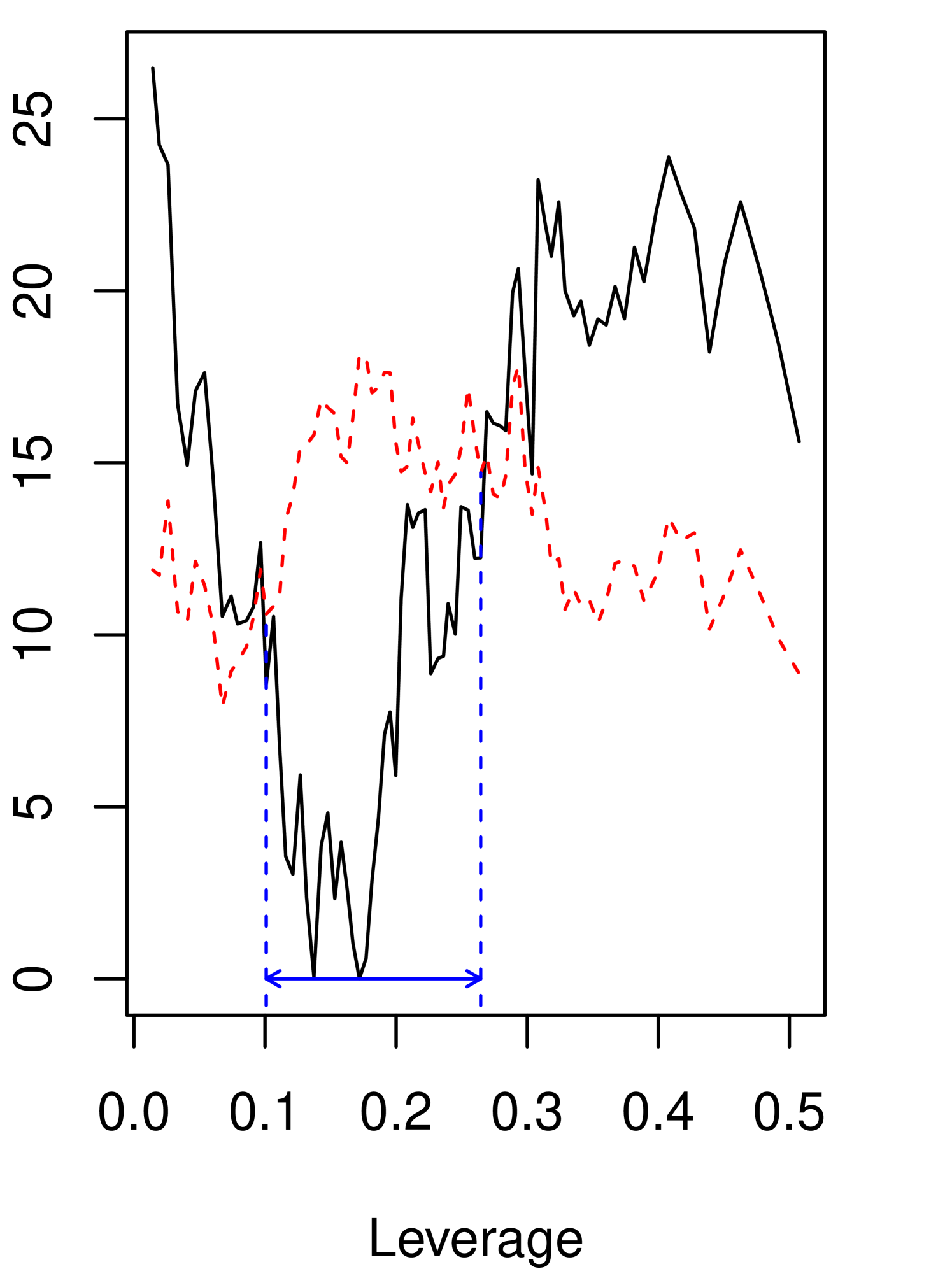
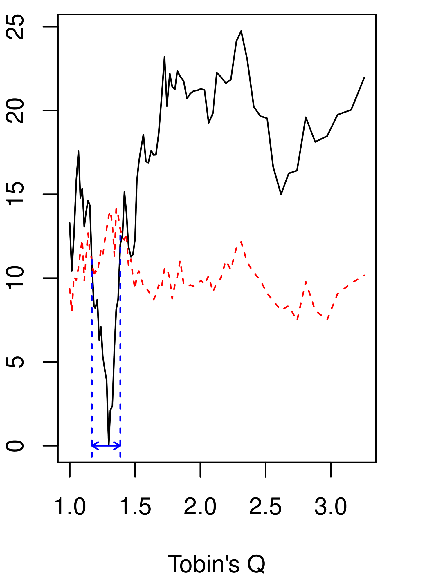
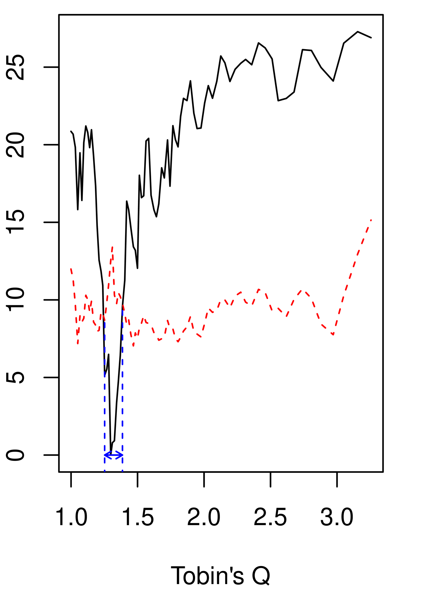
We find supporting evidence for the presence of the threshold effect when the threshold variable is Tobin’s Q, but the statistical evidence is not strong for the leverage threshold model. Table 5 and Table 6 report the bootstrap p-values at .135, .011, and .011, for specifications (16) - (18), respectively. The statistical evidence to reject the continuity is not trivial for all specifications and gets stronger when it is the restricted model using Tobin’s Q. The estimated bootstrap p-values are .028 and .004 for the unrestricted and the restricted using Tobin’s Q. Furthermore, the confidence interval for the threshold location is narrower for the restricted model (18) than for the unrestricted model (17).

Table 5: Columns (a) and (b) report results of the models (16) and (17), respectively. The percentile of each threshold location value is shown in parentheses below each value. The significance levels for the coefficients are given by stars: * - 10%, ** - 5% and *** - 1%.
(a) (b)
est. [95% CI] est. [95% CI]
Lower regime Lower regime
It1I_{t-1} 0.778** 0.124 1.154 It1I_{t-1} 0.252 -0.258 0.724
CFt1CF_{t-1} 0.047 -0.034 0.145 CFt1CF_{t-1} 0.266* -0.003 0.535
PPEt1PPE_{t-1} -0.147 -0.385 0.171 PPEt1PPE_{t-1} 0.027 -0.103 0.264
ROAt1ROA_{t-1} -0.032 -0.132 0.047 ROAt1ROA_{t-1} -0.017 -0.180 0.090
LEVt1LEV_{t-1} 0.231 -0.843 1.849 TQt1TQ_{t-1} 0.246* -0.031 0.577
Upper regime Upper regime
It1I_{t-1} -0.154 -0.717 0.551 It1I_{t-1} 0.410 -0.049 0.751
CFt1CF_{t-1} 0.148 -0.015 0.326 CFt1CF_{t-1} 0.081** 0.021 0.200
PPEt1PPE_{t-1} -0.291* -0.519 0.015 PPEt1PPE_{t-1} 0.044 -0.214 0.398
ROAt1ROA_{t-1} 0.013 -0.066 0.113 ROAt1ROA_{t-1} 0.050* -0.019 0.153
LEVt1LEV_{t-1} -0.081 -0.234 0.037 TQt1TQ_{t-1} 0.005 -0.004 0.012
Difference between regimes Difference between regimes
intercept 0.068 -0.024 0.200 intercept 0.236* -0.014 0.580
It1I_{t-1} -0.932** -1.830 -0.097 It1I_{t-1} 0.158 -0.559 0.843
CFt1CF_{t-1} 0.101 -0.107 0.322 CFt1CF_{t-1} -0.185 -0.479 0.108
PPEt1PPE_{t-1} -0.144 -0.519 0.134 PPEt1PPE_{t-1} 0.017 -0.227 0.275
ROAt1ROA_{t-1} 0.045 -0.111 0.232 ROAt1ROA_{t-1} 0.066 -0.074 0.287
LEVt1LEV_{t-1} -0.312* -1.893 0.792 TQt1TQ_{t-1} -0.242* -0.573 0.038
Threshold Threshold
LEVt1LEV_{t-1} 0.172 0.101 0.265 TQt1TQ_{t-1} 1.298 1.169 1.386
(38%) (24%) (58%) (30%) (21%) (36%)
Testing (p-val) Testing (p-val)
Linearity 0.135 Linearity 0.011
Continuity 0.033 Continuity 0.028
Table 6: Results of the model (18) are reported. The percentile of each threshold location value is shown in parentheses below each value. The significance levels for the coefficients are given by stars: * - 10%, ** - 5% and *** - 1%.
est. [95% CI]
Coefficients
It1I_{t-1} 0.392*** 0.304 0.539
CFt1CF_{t-1} 0.122*** 0.084 0.154
PPEt1PPE_{t-1} 0.076 -0.027 0.271
ROAt1ROA_{t-1} 0.027*** 0.006 0.046
TQt11{TQt1γ}TQ_{t-1}1\{TQ_{t-1}\leq\gamma\} 0.298** 0.073 0.571
TQt11{TQt1>γ}TQ_{t-1}1\{TQ_{t-1}>\gamma\} 0.008** 0.001 0.015
Difference between regimes
intercept 0.275** 0.010 0.540
TQt1TQ_{t-1} -0.290** -0.562 -0.018
Threshold
TQt1TQ_{t-1} 1.298 1.253 1.386
(30%) (27%) (36%)
Testing (p-val)
Linearity 0.011
Continuity 0.004

A notable finding concerning the coefficients estimates is that the relationship between cash flow and investment is positive and has larger magnitude for the low Tobin’s Q firms and the high leverage firms compared to their other respective regimes, although they are not statistically significant at 5% level. Even though the sign and magnitude of the estimates align with the observations by Lang et al., (1996) and Hansen, 1999b that a firm is subject to financial constraints when its Tobin’s Q is low or leverage is high, there is uncertainty in the interpretation of our results due to the lack of statistical significance.

Next, the autoregressive coefficient of the lagged investment is significant at 5% level in the low leverage regime and is larger than in the high leverage regime. This lends supporting evidence for the presence of asymmetric dynamics in investment, akin to the dynamics of leverage analyzed by Dang et al., (2012). In the meantime, we note that the autoregressive coefficients for the low and high leverage regimes in Column (a) are 0.778 and -0.154, respectively, which appear more extreme than findings of the literature where the estimates are between 0.1 and 0.5, e.g., Blundell et al., (1992). The autoregressive coefficients in the Column (b) are more in line with these estimates. Since the changes of the estimated coefficients in Column (b) are moderate, we also estimate the restricted model (18).

Turning to Table 6, we observe that the differences between the coefficients of the two regimes become significant at 5% level, and the CI for the threshold location becomes narrower while the estimate of the threshold location remains close to the estimate under the unrestricted model. The autoregressive coefficient of the lagged investment and the sensitivity of investment to both cash flow and return on assets are all positive and significant. The effect of Tobin’s Q is both positive and significant for both high and low Tobin’s Q regimes, but it almost disappears once it surpasses the threshold location. This suggests that low Tobin’s Q is related to low investment but higher Tobin’s Q does not cause higher investment once it reaches some level.

7 Conclusion

This paper studies the asymptotic properties of the GMM estimator in dynamic panel threshold models, showing that the limiting distribution depends critically on whether the true model exhibits a kink or a jump at the threshold. We demonstrate that the standard nonparametric bootstrap is inconsistent when the true model has a kink. To address this, we propose alternative bootstrap procedures for constructing confidence intervals for the threshold location and the model coefficients, which are shown to be consistent regardless of the model’s continuity. In particular, we establish that the grid bootstrap for the threshold parameter is uniformly valid. Monte Carlo simulations confirm that the proposed methods outperform the standard bootstrap in finite samples.

Several directions remain for future research. Our simulation results reveal highly asymmetric bootstrap distributions for the coefficient estimates, which distort finite sample inference. This highlights the need for a more thorough theoretical understanding of the bootstrap’s behavior. In particular, establishing the uniform validity of the bootstrap for the coefficient estimates is an important open question. Extensions of our bootstrap algorithms to incorporate latent group structures, interactive fixed effects, or threshold indices, as studied in Miao et al., 2020b , Miao et al., 2020a , and Seo and Linton, (2007); Lee et al., (2021), respectively, would also be valuable.

References

  • Adam and Bevan, (2005) Adam, C. S. and Bevan, D. L. (2005). Fiscal deficits and growth in developing countries. Journal of Public Economics, 89:571–597.
  • Andrews et al., (2020) Andrews, D. W., Cheng, X., and Guggenberger, P. (2020). Generic results for establishing the asymptotic size of confidence sets and tests. Journal of Econometrics, 218(2):496–531.
  • Andrews, (2001) Andrews, D. W. K. (2001). Testing when a parameter is on the boundary of the maintained hypothesis. Econometrica, 69(3):683–734.
  • Andrews, (2002) Andrews, D. W. K. (2002). Generalized method of moments estimation when a parameter is on a boundary. Journal of Business & Economic Statistics, 20(4):530–544.
  • Andrews and Cheng, (2012) Andrews, D. W. K. and Cheng, X. (2012). Estimation and Inference With Weak, Semi-Strong, and Strong Identification. Econometrica, 80:2153–2211.
  • Andrews and Cheng, (2014) Andrews, D. W. K. and Cheng, X. (2014). GMM Estimation and Uniform Subvector Inference With Possible Identification Failure. Econometric Theory, 30:287–333.
  • Andrews and Guggenberger, (2009) Andrews, D. W. K. and Guggenberger, P. (2009). Hybrid and size-corrected subsampling methods. Econometrica, 77(3):721–762.
  • Andrews and Guggenberger, (2019) Andrews, D. W. K. and Guggenberger, P. (2019). Identification- and singularity-robust inference for moment condition models. Quantitative Economics, 10:1703–1746.
  • Arellano and Bond, (1991) Arellano, M. and Bond, S. (1991). Some Tests of Specification for Panel Data: Monte Carlo Evidence and an Application to Employment Equations. The Review of Economic Studies, 58:277–297.
  • Bick, (2010) Bick, A. (2010). Threshold effects of inflation on economic growth in developing countries. Economics Letters, 108(2):126–129.
  • Blundell et al., (1992) Blundell, R., Bond, S., Devereux, M., and Schiantarelli, F. (1992). Investment and Tobin’s Q: Evidence from company panel data. Journal of Econometrics, 51:233–257.
  • Boyd and Vandenberghe, (2004) Boyd, S. and Vandenberghe, L. (2004). Convex Optimization. Cambridge University Press.
  • Cavaliere et al., (2022) Cavaliere, G., Nielsen, H. B., Pedersen, R. S., and Rahbek, A. (2022). Bootstrap inference on the boundary of the parameter space, with application to conditional volatility models. Journal of Econometrics, 227(1):241–263.
  • Cecchetti et al., (2011) Cecchetti, S. G., Mohanty, M. S., and Zampolli, F. (2011). The Real Effects of Debt. BIS Working Paper No. 352.
  • Chan and Tong, (1985) Chan, K. S. and Tong, H. (1985). On the use of the deterministic lyapunov function for the ergodicity of stochastic difference equations. Advances in applied probability, 17(3):666–678.
  • Chan and Tsay, (1998) Chan, K. S. and Tsay, R. S. (1998). Limiting properties of the least squares estimator of a continuous threshold autoregressive model. Biometrika, 85(2):413–426.
  • Chatterjee and Lahiri, (2011) Chatterjee, A. and Lahiri, S. N. (2011). Bootstrapping lasso estimators. Journal of the American Statistical Association, 106(494):608–625.
  • Cheng and Huang, (2010) Cheng, G. and Huang, J. Z. (2010). Bootstrap consistency for general semiparametric m-estimation. The Annals of Statistics, 38(5):2884–2915.
  • Chudik et al., (2017) Chudik, A., Mohaddes, K., Pesaran, M. H., and Raissi, M. (2017). Is There a Debt-Threshold Effect on Output Growth? The Review of Economics and Statistics, 99:135–150.
  • Dang et al., (2012) Dang, V. A., Kim, M., and Shin, Y. (2012). Asymmetric capital structure adjustments: New evidence from dynamic panel threshold models. Journal of Empirical Finance, 19:465–482.
  • Dovonon and Goncalves, (2017) Dovonon, P. and Goncalves, S. (2017). Bootstrapping the GMM overidentification test under first-order underidentification. Journal of Econometrics, 201:43–71.
  • Dovonon and Hall, (2018) Dovonon, P. and Hall, A. R. (2018). The asymptotic properties of gmm and indirect inference under second-order identification. Journal of Econometrics, 205(1):76–111.
  • Dovonon and Renault, (2013) Dovonon, P. and Renault, E. (2013). Testing for Common Conditionally Heteroskedastic Factors. Econometrica, 81:2561–2586.
  • Fazzari et al., (1988) Fazzari, S. M., Hubbard, R. G., Petersen, B. C., Blinder, A. S., and Poterba, J. M. (1988). Financing Constraints and Corporate Investment. Brookings Papers on Economic Activity, 1988:141–206.
  • Giannerini et al., (2024) Giannerini, S., Goracci, G., and Rahbek, A. (2024). The validity of bootstrap testing for threshold autoregression. Journal of Econometrics, 239(1):105379.
  • Gine and Zinn, (1990) Gine, E. and Zinn, J. (1990). Bootstrapping general empirical measures. The Annals of Probability, 18(2):851 – 869.
  • Girma, (2005) Girma, S. (2005). Absorptive Capacity and Productivity Spillovers from FDI: A Threshold Regression Analysis. Oxford Bulletin of Economics and Statistics, 67:281–306.
  • Goncalves and White, (2004) Goncalves, S. and White, H. (2004). Maximum likelihood and the bootstrap for nonlinear dynamic models. Journal of Econometrics, 119(1):199–219.
  • Gonzalo and Wolf, (2005) Gonzalo, J. and Wolf, M. (2005). Subsampling inference in threshold autoregressive models. Journal of Econometrics, 127(2):201–224.
  • Hall and Horowitz, (1996) Hall, P. and Horowitz, J. L. (1996). Bootstrap Critical Values for Tests Based on Generalized-Method-of-Moments Estimators. Econometrica, 64:891–916.
  • Han and McCloskey, (2019) Han, S. and McCloskey, A. (2019). Estimation and Inference with a (nearly) Singular Jacobian. Quantitative Economics, 10:1019–1068.
  • (32) Hansen, B. E. (1999a). The Grid Bootstrap and the Autoregressive Model. The Review of Economics and Statistics, 81:594–607.
  • (33) Hansen, B. E. (1999b). Threshold effects in non-dynamic panels: Estimation, testing, and inference. Journal of Econometrics, 93:345–368.
  • Hansen, (2000) Hansen, B. E. (2000). Sample Splitting and Threshold Estimation. Econometrica, 68:575–603.
  • Hansen, (2017) Hansen, B. E. (2017). Regression kink with an unknown threshold. Journal of Business & Economic Statistics, 35(2):228–240.
  • Hidalgo et al., (2023) Hidalgo, J., Lee, H., Lee, J., and Seo, M. H. (2023). Minimax risk in estimating kink threshold and testing continuity. In Advances in Econometrics: Essays in Honor of Joon Y. Park: Econometric Theory, Vol. 45A, pages 233–259.
  • Hidalgo et al., (2019) Hidalgo, J., Lee, J., and Seo, M. H. (2019). Robust Inference for Threshold Regression Models. Journal of Econometrics, 210:291–309.
  • Khan and Senhadji, (2001) Khan, M. S. and Senhadji, A. S. (2001). Threshold Effects in the Relationship between Inflation and Growth. IMF Staff Papers, 48:1–21.
  • Kim et al., (2019) Kim, S., Kim, Y. J., and Seo, M. H. (2019). Estimation of Dynamic Panel Threshold Model Using Stata. The Stata Journal, 19:685–697.
  • Kremer et al., (2013) Kremer, S., Bick, A., and Nautz, D. (2013). Inflation and growth: new evidence from a dynamic panel threshold analysis. Empirical Economics, 44:861–878.
  • Lang et al., (1996) Lang, L., Ofek, E., and Stulz, R. (1996). Leverage, investment, and firm growth. Journal of Financial Economics, 40(1):3–29.
  • Lee et al., (2021) Lee, S., Liao, Y., Seo, M. H., and Shin, Y. (2021). Factor-driven two-regime regression. The Annals of Statistics, 49(3):1656–1678.
  • Lee et al., (2011) Lee, S., Seo, M. H., and Shin, Y. (2011). Testing for Threshold Effects in Regression Models. Journal of the American Statistical Association, 106:220–231.
  • Leeb and Pötscher, (2005) Leeb, H. and Pötscher, B. M. (2005). Model selection and inference: facts and fiction. Econometric Theory, 21(1):21–59.
  • (45) Miao, K., Li, K., and Su, L. (2020a). Panel threshold models with interactive fixed effects. Journal of Econometrics, 219(1):137–170.
  • (46) Miao, K., Su, L., and Wang, W. (2020b). Panel threshold regressions with latent group structures. Journal of Econometrics, 214(2):451–481.
  • Mikusheva, (2007) Mikusheva, A. (2007). Uniform inference in autoregressive models. Econometrica, 75(5):1411–1452.
  • Newey and McFadden, (1994) Newey, W. K. and McFadden, D. (1994). Chapter 36 Large Sample Estimation and Hypothesis Testing. In Handbook of Econometrics, volume 4, pages 2111–2245. Elsevier.
  • Newey and West, (1987) Newey, W. K. and West, K. D. (1987). Hypothesis Testing with Efficient Method of Moments Estimation. International Economic Review, 28:777–787.
  • Pakes and Pollard, (1989) Pakes, A. and Pollard, D. (1989). Simulation and the Asymptotics of Optimization Estimators. Econometrica, 57:1027–1057.
  • Praestgaard and Wellner, (1993) Praestgaard, J. and Wellner, J. A. (1993). Exchangeably Weighted Bootstraps of the General Empirical Process. The Annals of Probability, 21(4):2053 – 2086.
  • Romano and Shaikh, (2012) Romano, J. P. and Shaikh, A. M. (2012). On the uniform asymptotic validity of subsampling and the bootstrap. The Annals of Statistics, 40(6):2798 – 2822.
  • Rousseau and Wachtel, (2002) Rousseau, P. L. and Wachtel, P. (2002). Inflation thresholds and the finance–growth nexus. Journal of International Money and Finance, 21:777–793.
  • Seo and Linton, (2007) Seo, M. H. and Linton, O. (2007). A smoothed least squares estimator for threshold regression models. Journal of Econometrics, 141(2):704–735.
  • Seo and Shin, (2016) Seo, M. H. and Shin, Y. (2016). Dynamic Panels With Threshold Effect and Endogeneity. Journal of Econometrics, 195:169–186.
  • Strebulaev and Yang, (2013) Strebulaev, I. A. and Yang, B. (2013). The mystery of zero-leverage firms. Journal of Financial Economics, 109(1):1–23.
  • van der Vaart and Wellner, (1996) van der Vaart, A. W. and Wellner, J. (1996). Weak Convergence and Empirical Processes With Applications to Statistics. Springer Series in Statistics. Springer-Verlag, New York.
  • Wang, (2015) Wang, Q. (2015). Fixed-effect panel threshold model using stata. The Stata Journal, 15(1):121–134.
  • Yang et al., (2020) Yang, L., Zhang, C., Lee, C., and Chen, I.-P. (2020). Panel kink threshold regression model with a covariate-dependent threshold. The Econometrics Journal, 24(3):462–481.
  • Zhang et al., (2017) Zhang, Y., Zhou, Q., and Jiang, L. (2017). Panel kink regression with an unknown threshold. Economics Letters, 157:116–121.
Additional Notations.

For k,pk,p\in\mathbb{N}, 0k×p0_{k\times p} denotes k×pk\times p a matrix whose elements are all zero. “\rightsquigarrow” denotes the weak convergence as in section 1.3 of van der Vaart and Wellner, (1996). \|\cdot\| is a norm for either vectors or matrices. For a vector, it is the Euclidean norm. For a matrix, it is the Frobenius norm, i.e., M=tr(MM)\|M\|=\sqrt{tr(M^{\prime}M)} for a matrix MM.

Appendix A Proofs for Section 3.

A.1 Proof of Theorem 1.

Note that E[zit(ΔyitΔxitβ1it(γ)Xitδ)]=E[zitΔxit](ββ0)E[zit1it(γ)Xit]δ+E[zit1it(γ0)Xitδ0]E[z_{it}(\Delta y_{it}-\Delta x_{it}^{\prime}\beta-1_{it}(\gamma)^{\prime}X_{it}\delta)]=-E[z_{it}\Delta x_{it}^{\prime}](\beta-\beta_{0})-E[z_{it}1_{it}(\gamma)^{\prime}X_{it}]\delta+E[z_{it}1_{it}(\gamma_{0})^{\prime}X_{it}\delta_{0}] due to Δyit=Δxitβ0+1it(γ0)Xitδ0+Δϵit\Delta y_{it}=\Delta x_{it}^{\prime}\beta_{0}+1_{it}(\gamma_{0})^{\prime}X_{it}\delta_{0}+\Delta\epsilon_{it}. Hence, the population moment equation is g0(θ)=M10(ββ0)+M20(γ)δM20δ0=[M0(γ)M_20δ_0]×((ββ0,δ),1),g_{0}(\theta)=M_{10}(\beta-\beta_{0})+M_{20}(\gamma)\delta-M_{20}\delta_{0}=\left[\begin{array}[]{c;{2pt/2pt}c}M_{0}(\gamma)&M_{20}\delta_{0}\\ \end{array}\right]\times((\beta^{\prime}-\beta_{0}^{\prime},\delta^{\prime}),-1)^{\prime}, when γγ0\gamma\neq\gamma_{0}. The condition (ii) of Theorem 1 implies that [M0(γ)M_20δ_0]\left[\begin{array}[]{c;{2pt/2pt}c}M_{0}(\gamma)&M_{20}\delta_{0}\\ \end{array}\right] has full column rank, and hence g0(θ)0kg_{0}(\theta)\neq 0_{k} if γγ0\gamma\neq\gamma_{0}. g0(θ)=M0×(αα0)g_{0}(\theta)=M_{0}\times(\alpha-\alpha_{0}), when γ=γ0\gamma=\gamma_{0}. The condition (i) of Theorem 1 implies that M0×(αα0)M_{0}\times(\alpha-\alpha_{0}) is not zero if αα0\alpha\neq\alpha_{0}. Therefore, g0(θ)0kg_{0}(\theta)\neq 0_{k} if θθ0\theta\neq\theta_{0}, and g0(θ)=0kg_{0}(\theta)=0_{k} if θ=θ0\theta=\theta_{0}, which is the standard identification condition in the literature, e.g., Section 2.2.3 in Newey and McFadden, (1994).

A.2 Proof of Theorem 2.

To obtain limit distribution of θ^\hat{\theta}, we first establish consistency of θ^\hat{\theta} to θ0\theta_{0} and rate of θ^\hat{\theta}’s convergence. Then, we show asymptotic distribution of the estimates using rescaled versions of the parameters and criterions.

A.2.1 Consistency.

Constrained estimator of the coefficients, α^(γ)=argminαAQ^n(α,γ)\hat{\alpha}(\gamma)=\arg\min_{\alpha\in A}\hat{Q}_{n}(\alpha,\gamma), given a fixed γ\gamma can be expressed as

α^(γ)=(M¯n(γ)WnM¯n(γ))1M¯n(γ)Wnv¯n\hat{\alpha}(\gamma)=-(\bar{M}_{n}(\gamma)^{\prime}W_{n}\bar{M}_{n}(\gamma))^{-1}\bar{M}_{n}(\gamma)^{\prime}W_{n}\bar{v}_{n}

where

v¯n=M¯nα0+un,un=1ni=1n(zit0Δϵit0ziTΔϵiT).\bar{v}_{n}=-\bar{M}_{n}\alpha_{0}+u_{n},\quad u_{n}=\frac{1}{n}\sum_{i=1}^{n}\begin{pmatrix}z_{it_{0}}\Delta\epsilon_{it_{0}}\\ \vdots\\ z_{iT}\Delta\epsilon_{iT}\end{pmatrix}.

Therefore,

α^(γ)=(M¯n(γ)WnM¯n(γ))1M¯n(γ)Wn(M¯nα0+un).\hat{\alpha}(\gamma)=-(\bar{M}_{n}(\gamma)^{\prime}W_{n}\bar{M}_{n}(\gamma))^{-1}\bar{M}_{n}(\gamma)^{\prime}W_{n}(-\bar{M}_{n}\alpha_{0}+u_{n}).

Define profiled criterion with respect to γ\gamma by g~n(γ)=g¯n(α^(γ),γ)\tilde{g}_{n}(\gamma)=\bar{g}_{n}(\hat{\alpha}(\gamma),\gamma) and Q~n(γ)=g~n(γ)Wng~n(γ)\tilde{Q}_{n}(\gamma)=\tilde{g}_{n}(\gamma)^{\prime}W_{n}\tilde{g}_{n}(\gamma). The threshold location estimator is γ^=argminγΓg~n(γ)Wng~n(γ)\hat{\gamma}=\arg\min_{\gamma\in\Gamma}\tilde{g}_{n}(\gamma)^{\prime}W_{n}\tilde{g}_{n}(\gamma). By the law of large numbers (LLN), un𝑝0u_{n}\xrightarrow{p}0. By the uniform law of large numbers (ULLN) in Lemma D.2, M¯n(γ)𝑝M0(γ)\bar{M}_{n}(\gamma)\xrightarrow{p}M_{0}(\gamma) uniformly with respect to γΓ\gamma\in\Gamma. Hence, γ^𝑝γ0\hat{\gamma}\xrightarrow{p}\gamma_{0} would imply M¯n(γ^)𝑝M0\bar{M}_{n}(\hat{\gamma})\xrightarrow{p}M_{0}, and then α^(γ^)𝑝α0\hat{\alpha}(\hat{\gamma})\xrightarrow{p}\alpha_{0}, which completes the proof.

To show consistency of γ^\hat{\gamma} to γ0\gamma_{0}, we apply the argmin/argmax continuous mapping theorem (CMT) as in Theorem 3.2.2 in van der Vaart and Wellner, (1996). It is sufficient to check (i) Q~n(γ)\tilde{Q}_{n}(\gamma) uniformly converges to some function Q~0(γ)\tilde{Q}_{0}(\gamma) in probability, and (ii) Q~0(γ0)<infγ𝒪Q~0(γ)\tilde{Q}_{0}(\gamma_{0})<\inf_{\gamma\not\in\mathcal{O}}\tilde{Q}_{0}(\gamma) for any open set 𝒪\mathcal{O} contatining γ0\gamma_{0}. (ii) can be shown if Q~0(γ)\tilde{Q}_{0}(\gamma) is uniquely minimized at γ0\gamma_{0} and continuous as Γ\Gamma is compact.

The profiled moment can be rewritten as

g~n(γ)=[IM¯n(γ)(M¯n(γ)WnM¯n(γ))1M¯n(γ)Wn](M¯nα0+un).\tilde{g}_{n}(\gamma)=[I-\bar{M}_{n}(\gamma)\left(\bar{M}_{n}(\gamma)^{\prime}W_{n}\bar{M}_{n}(\gamma)\right)^{-1}\bar{M}_{n}(\gamma)^{\prime}W_{n}](-\bar{M}_{n}\alpha_{0}+u_{n}).

Therefore,

Wn1/2g~n(γ)=[IPWn1/2M¯n(γ)](Wn1/2M¯nα0+Wn1/2un),W_{n}^{1/2}\tilde{g}_{n}(\gamma)=[I-P_{W_{n}^{1/2}\bar{M}_{n}(\gamma)}](-W_{n}^{1/2}\bar{M}_{n}\alpha_{0}+W_{n}^{1/2}u_{n}),

where PWn1/2M¯n(γ)=Wn1/2M¯n(γ)(M¯n(γ)WnM¯n(γ))1M¯n(γ)Wn1/2P_{W_{n}^{1/2}\bar{M}_{n}(\gamma)}=W_{n}^{1/2}\bar{M}_{n}(\gamma)\left(\bar{M}_{n}(\gamma)^{\prime}W_{n}\bar{M}_{n}(\gamma)\right)^{-1}\bar{M}_{n}(\gamma)^{\prime}W_{n}^{1/2} is a projection matrix to the column space of Wn1/2M¯n(γ)W_{n}^{1/2}\bar{M}_{n}(\gamma). The profiled objective can be written as

Q~n(γ)=(IPWn1/2M¯n(γ))(Wn1/2M¯nα0+Wn1/2un)2.\tilde{Q}_{n}(\gamma)=\|(I-P_{W_{n}^{1/2}\bar{M}_{n}(\gamma)})(-W_{n}^{1/2}\bar{M}_{n}\alpha_{0}+W_{n}^{1/2}u_{n})\|^{2}.

By Wn𝑝WW_{n}\xrightarrow{p}W, un𝑝0u_{n}\xrightarrow{p}0, and supγΓM¯n(γ)M0(γ)𝑝0\sup_{\gamma\in\Gamma}\|\bar{M}_{n}(\gamma)-M_{0}(\gamma)\|\xrightarrow{p}0, we can derive that

Q~n(γ)𝑝Q~0(γ)=(IPW1/2M0(γ))W1/2M0α02\tilde{Q}_{n}(\gamma)\xrightarrow{p}\tilde{Q}_{0}(\gamma)=\|(I-P_{W^{1/2}M_{0}(\gamma)})W^{1/2}M_{0}\alpha_{0}\|^{2}

uniformly with respect to γ\gamma, where PW1/2M0(γ)=W1/2M0(γ)(M0(γ)WM0(γ))1M0(γ)W1/2P_{W^{1/2}M_{0}(\gamma)}=W^{1/2}M_{0}(\gamma)\left(M_{0}(\gamma)^{\prime}WM_{0}(\gamma)\right)^{-1}M_{0}(\gamma)^{\prime}W^{1/2}. Note that W=Ω1W=\Omega^{-1} in the second stage of the two-step GMM estimation. W=IW=I when we consider the first stage. Q~0(γ)\tilde{Q}_{0}(\gamma) is uniquely minimized when γ=γ0\gamma=\gamma_{0}. This is because WW is positive definite, and the conditions in Theorem 1 implies that M0α0M_{0}\alpha_{0} does not lie in the column space of M0(γ)M_{0}(\gamma) whenever γγ0\gamma\neq\gamma_{0}. Moreover, Q~0(γ)\tilde{Q}_{0}(\gamma) is continuous as M0(γ)M_{0}(\gamma) is continuous with respect to γ\gamma by D.

A.2.2 Convergence rate.

WnΩ1𝑝0\|W_{n}-\Omega^{-1}\|\xrightarrow{p}0 as the consistency of θ^(1)\hat{\theta}_{(1)} is shown. Our proof follows arguments similar to the proof of Theorem 3.3 by Pakes and Pollard, (1989). By the consistency of θ^\hat{\theta} and by Lemma D.3,

ng¯n(θ^)g¯n(θ0)g0(θ^)=op(1).\sqrt{n}\|\bar{g}_{n}(\hat{\theta})-\bar{g}_{n}(\theta_{0})-g_{0}(\hat{\theta})\|=o_{p}(1).

By WnΩ1𝑝0\|W_{n}-\Omega^{-1}\|\xrightarrow{p}0, we can obtain

nWn1/2g¯n(θ^)Wn1/2g¯n(θ0)Ω1/2g0(θ^)=op(1).\sqrt{n}\|W_{n}^{1/2}\bar{g}_{n}(\hat{\theta})-W_{n}^{1/2}\bar{g}_{n}(\theta_{0})-\Omega^{-1/2}g_{0}(\hat{\theta})\|=o_{p}(1).

Apply triangle inequality to get

nΩ1/2g0(θ^)op(1)+nWn1/2g¯n(θ0)+nWn1/2g¯n(θ^).\sqrt{n}\|\Omega^{-1/2}g_{0}(\hat{\theta})\|\leq o_{p}(1)+\sqrt{n}\|W_{n}^{1/2}\bar{g}_{n}(\theta_{0})\|+\sqrt{n}\|W_{n}^{1/2}\bar{g}_{n}(\hat{\theta})\|.

As θ^\hat{\theta} is the minimizer of the GMM criterion, nWn1/2g¯n(θ^)op(1)+nWn1/2g¯n(θ0)=Op(1)\sqrt{n}\|W_{n}^{1/2}\bar{g}_{n}(\hat{\theta})\|\leq o_{p}(1)+\sqrt{n}\|W_{n}^{1/2}\bar{g}_{n}(\theta_{0})\|=O_{p}(1). Therefore,

nΩ1/2g0(θ^)Op(1).\sqrt{n}\|\Omega^{-1/2}g_{0}(\hat{\theta})\|\leq O_{p}(1).

nΩ1/2g0(θ^)nΩ1/2D2(α^α0,(γ^γ0)2)nΩ1/2(g(θ^)D2(α^α0,(γ^γ0)2))\sqrt{n}\|\Omega^{-1/2}g_{0}(\hat{\theta})\|\geq\sqrt{n}\|\Omega^{-1/2}D_{2}(\hat{\alpha}^{\prime}-\alpha_{0}^{\prime},(\hat{\gamma}-\gamma_{0})^{2})^{\prime}\|-\sqrt{n}\|\Omega^{-1/2}(g(\hat{\theta})-D_{2}(\hat{\alpha}^{\prime}-\alpha_{0}^{\prime},(\hat{\gamma}-\gamma_{0})^{2})^{\prime})\|, while nΩ1/2(g(θ^)D2(α^α0,(γ^γ0)2))op(1+n(α^α0,(γ^γ0)2))\sqrt{n}\|\Omega^{-1/2}(g(\hat{\theta})-D_{2}(\hat{\alpha}^{\prime}-\alpha_{0}^{\prime},(\hat{\gamma}-\gamma_{0})^{2})^{\prime})\|\leq o_{p}(1+\sqrt{n}\|(\hat{\alpha}^{\prime}-\alpha_{0}^{\prime},(\hat{\gamma}-\gamma_{0})^{2})^{\prime}\|) by Lemma D.1. Thus,

n(α^α0+(γ^γ0)2)Op(1)\sqrt{n}(\|\hat{\alpha}-\alpha_{0}\|+(\hat{\gamma}-\gamma_{0})^{2})\leq O_{p}(1)

which implies α^α0=Op(n1/2)\|\hat{\alpha}-\alpha_{0}\|=O_{p}(n^{-1/2}) and (γ^γ0)2=Op(n1/2)(\hat{\gamma}-\gamma_{0})^{2}=O_{p}(n^{-1/2}).

A.2.3 Asymptotic distribution.

This section derives asymptotic distribution of the estimator through the argmin/argmax continuous mapping theorem (CMT) as in Theorem 3.2.2 in van der Vaart and Wellner, (1996).

Introduce a local reparametrization by a=n(αα0)a=\sqrt{n}(\alpha-\alpha_{0}) and b=n14(γγ0)b=n^{\frac{1}{4}}(\gamma-\gamma_{0}), and let aa consist of subvectors a1=n(ββ0)a_{1}=\sqrt{n}(\beta-\beta_{0}) and a2=n(δδ0)a_{2}=\sqrt{n}(\delta-\delta_{0}). Additionally, define a^=n(α^α0)\hat{a}=\sqrt{n}(\hat{\alpha}-\alpha_{0}) and b^=n14(γ^γ0)\hat{b}=n^{\frac{1}{4}}(\hat{\gamma}-\gamma_{0}). Note that (a^,b^2)(\hat{a},\hat{b}^{2}) is uniformly tight due to the convergence rate we obtained.333 A random variable XX is tight if for any ϵ>0\epsilon>0, there exists a compact set 𝕂\mathbb{K} such that P(X𝕂)>1ϵP(X\in\mathbb{K})>1-\epsilon, and XnX_{n} is uniformly tight if for any ϵ>0\epsilon>0, there exists a compact set 𝕂\mathbb{K} such that P(Xn𝕂)>1ϵP(X_{n}\in\mathbb{K})>1-\epsilon for all nn\in\mathbb{N}. Note that by the convergence rate we derived, for any ϵ>0\epsilon>0, there exists a compact 𝕂0\mathbb{K}_{0} such that limnP((n(α^α0),n(γ^γ0)2)𝕂0)>1ϵ/2\lim_{n\rightarrow\infty}P((\sqrt{n}(\hat{\alpha}-\alpha_{0})^{\prime},\sqrt{n}(\hat{\gamma}-\gamma_{0})^{2})^{\prime}\in\mathbb{K}_{0})>1-\epsilon/2, and N<N<\infty such that P((n(α^α0),n(γ^γ0)2)𝕂0)>1ϵP((\sqrt{n}(\hat{\alpha}-\alpha_{0})^{\prime},\sqrt{n}(\hat{\gamma}-\gamma_{0})^{2})^{\prime}\in\mathbb{K}_{0})>1-\epsilon if nNn\geq N. Then, we can define a compact set 𝕂=(j=1N1𝕂j)𝕂0\mathbb{K}=(\cup_{j=1}^{N-1}\mathbb{K}_{j})\cup\mathbb{K}_{0}, where 𝕂j\mathbb{K}_{j} is a compact set such that P((j(α^α0),j(γ^γ0)2)𝕂j)>1ϵP((\sqrt{j}(\hat{\alpha}-\alpha_{0})^{\prime},\sqrt{j}(\hat{\gamma}-\gamma_{0})^{2})^{\prime}\in\mathbb{K}_{j})>1-\epsilon, which satisfies P((n(α^α0),n(γ^γ0)2)𝕂)>1ϵP((\sqrt{n}(\hat{\alpha}-\alpha_{0})^{\prime},\sqrt{n}(\hat{\gamma}-\gamma_{0})^{2})^{\prime}\in\mathbb{K})>1-\epsilon for all nn\in\mathbb{N}. Let

𝕊n(a,b)=nQ^n(α0+an,γ0+bn14)=ng¯n(α0+an,γ0+bn14)Wng¯n(α0+an,γ0+bn14).\mathbb{S}_{n}(a,b)=n\hat{Q}_{n}(\alpha_{0}+\tfrac{a}{\sqrt{n}},\gamma_{0}+\tfrac{b}{n^{\frac{1}{4}}})=n\bar{g}_{n}(\alpha_{0}+\tfrac{a}{\sqrt{n}},\gamma_{0}+\tfrac{b}{n^{\frac{1}{4}}})^{\prime}W_{n}\bar{g}_{n}(\alpha_{0}+\tfrac{a}{\sqrt{n}},\gamma_{0}+\tfrac{b}{n^{\frac{1}{4}}}).

We show that (i) 𝕊n\mathbb{S}_{n} weakly converges to a stochastic process 𝕊\mathbb{S} in (𝕂)\ell^{\infty}(\mathbb{K}) for every compact 𝕂\mathbb{K} in the Euclidean space, (ii) 𝕊\mathbb{S} is continuous, and (iii) 𝕊\mathbb{S} possesses an unique optimum not in bb but in its square b2b^{2} since 𝕊(a,b)=𝕊(a,b)\mathbb{S}(a,b)=\mathbb{S}(a,-b). Thus, we will establish that (a^,b^2)(\hat{a}^{\prime},\hat{b}^{2})^{\prime} converges in distribution to (a0,b02)=argmina,b2𝕊(a,b2)(a_{0}^{\prime},b_{0}^{2})^{\prime}=\arg\min_{a,b^{2}}\mathbb{S}(a,\sqrt{b^{2}}). In the characterization of the minimizers, (a0,b02)(a_{0}^{\prime},b_{0}^{2})^{\prime} is shown to be tight.

The rescaled and reparametrized sample moment can be written as

ng¯n(α0+an,γ0+bn14)=n(1ni=1nzit0Δϵit01ni=1nziTΔϵiT)(1ni=1nzit0Δxit01ni=1nziTΔxiT)a1(1ni=1nzit01it0(γ0+bn14)Xit01ni=1nziT1iT(γ0+bn14)XiT)a2+(1ni=1nzit0(1it0(γ0)1it0(γ0+bn14))Xit01ni=1nziT(1iT(γ0)1iT(γ0+bn14))XiT)δ0.\sqrt{n}\bar{g}_{n}(\alpha_{0}+\tfrac{a}{\sqrt{n}},\gamma_{0}+\tfrac{b}{n^{\frac{1}{4}}})=\sqrt{n}\begin{pmatrix}\frac{1}{n}\sum_{i=1}^{n}z_{it_{0}}\Delta\epsilon_{it_{0}}\\ \vdots\\ \frac{1}{n}\sum_{i=1}^{n}z_{iT}\Delta\epsilon_{iT}\end{pmatrix}-\begin{pmatrix}\tfrac{1}{n}\sum_{i=1}^{n}z_{it_{0}}\Delta x_{it_{0}}^{\prime}\\ \vdots\\ \tfrac{1}{n}\sum_{i=1}^{n}z_{iT}\Delta x_{iT}^{\prime}\end{pmatrix}a_{1}\\ -\begin{pmatrix}\tfrac{1}{n}\sum_{i=1}^{n}z_{it_{0}}1_{it_{0}}(\gamma_{0}+\tfrac{b}{n^{\frac{1}{4}}})^{\prime}X_{it_{0}}\\ \vdots\\ \tfrac{1}{n}\sum_{i=1}^{n}z_{iT}1_{iT}(\gamma_{0}+\tfrac{b}{n^{\frac{1}{4}}})^{\prime}X_{iT}\end{pmatrix}a_{2}+\begin{pmatrix}\tfrac{1}{\sqrt{n}}\sum_{i=1}^{n}z_{it_{0}}(1_{it_{0}}(\gamma_{0})^{\prime}-1_{it_{0}}(\gamma_{0}+\tfrac{b}{n^{\frac{1}{4}}})^{\prime})X_{it_{0}}\\ \vdots\\ \tfrac{1}{\sqrt{n}}\sum_{i=1}^{n}z_{iT}(1_{iT}(\gamma_{0})^{\prime}-1_{iT}(\gamma_{0}+\tfrac{b}{n^{\frac{1}{4}}})^{\prime})X_{iT}\end{pmatrix}\delta_{0}.

By the central limit theorem (CLT),

n(1ni=1nzit0Δϵit01ni=1nziTΔϵiT)𝑑eN(0,Ω).\sqrt{n}\begin{pmatrix}\frac{1}{n}\sum_{i=1}^{n}z_{it_{0}}\Delta\epsilon_{it_{0}}\\ \vdots\\ \frac{1}{n}\sum_{i=1}^{n}z_{iT}\Delta\epsilon_{iT}\end{pmatrix}\xrightarrow{d}-e\sim N(0,\Omega).

By the LLN,

(1ni=1nzit0Δxit01ni=1nziTΔxiT)𝑝(Ezit0Δxit0EziTΔxiT)\begin{pmatrix}\tfrac{1}{n}\sum_{i=1}^{n}z_{it_{0}}\Delta x_{it_{0}}^{\prime}\\ \vdots\\ \tfrac{1}{n}\sum_{i=1}^{n}z_{iT}\Delta x_{iT}^{\prime}\end{pmatrix}\xrightarrow{p}\begin{pmatrix}Ez_{it_{0}}\Delta x_{it_{0}}^{\prime}\\ \vdots\\ Ez_{iT}\Delta x_{iT}^{\prime}\end{pmatrix}

Let K<K<\infty be arbitrary. By the ULLN in Lemma D.2,

(1ni=1nzit01it0(γ0+bn14)Xit01ni=1nziT1iT(γ0+bn14)XiT)(Ezit01it0(γ0+bn14)Xit0EziT1iT(γ0+bn14)XiT)𝑝0\left\|\begin{pmatrix}\tfrac{1}{n}\sum_{i=1}^{n}z_{it_{0}}1_{it_{0}}(\gamma_{0}+\tfrac{b}{n^{\frac{1}{4}}})^{\prime}X_{it_{0}}\\ \vdots\\ \tfrac{1}{n}\sum_{i=1}^{n}z_{iT}1_{iT}(\gamma_{0}+\tfrac{b}{n^{\frac{1}{4}}})^{\prime}X_{iT}\end{pmatrix}-\begin{pmatrix}Ez_{it_{0}}1_{it_{0}}(\gamma_{0}+\tfrac{b}{n^{\frac{1}{4}}})^{\prime}X_{it_{0}}\\ \vdots\\ Ez_{iT}1_{iT}(\gamma_{0}+\tfrac{b}{n^{\frac{1}{4}}})^{\prime}X_{iT}\end{pmatrix}\right\|\xrightarrow{p}0

uniformly with respect to b[K,K]b\in[-K,K]. Then, by continuity of κE[zit1it(γ+κ)Xit]\kappa\mapsto E[z_{it}1_{it}(\gamma+\kappa)X_{it}] at κ=0\kappa=0,

(1ni=1nzit01it0(γ0+bn14)Xit01ni=1nziT1iT(γ0+bn14)XiT)𝑝(Ezit01it0(γ0)Xit0EziT1iT(γ0)XiT)\begin{pmatrix}\tfrac{1}{n}\sum_{i=1}^{n}z_{it_{0}}1_{it_{0}}(\gamma_{0}+\tfrac{b}{n^{\frac{1}{4}}})^{\prime}X_{it_{0}}\\ \vdots\\ \tfrac{1}{n}\sum_{i=1}^{n}z_{iT}1_{iT}(\gamma_{0}+\tfrac{b}{n^{\frac{1}{4}}})^{\prime}X_{iT}\end{pmatrix}\xrightarrow{p}\begin{pmatrix}Ez_{it_{0}}1_{it_{0}}(\gamma_{0})^{\prime}X_{it_{0}}\\ \vdots\\ Ez_{iT}1_{iT}(\gamma_{0})^{\prime}X_{iT}\end{pmatrix}

uniformly with respect to b[K,K]b\in[-K,K]. By Lemma D.4,

(1ni=1nzit0(1it0(γ0)1it0(γ0+bn14))Xit0δ01ni=1nziT(1iT(γ0)1iT(γ0+bn14))XiTδ0)𝑝δ302(Et0[zit0|γ0]ft0(γ0)Et01[zit0|γ0]ft01(γ0)ET[ziT|γ0]fT(γ0)ET1[ziT|γ0]fT1(γ0))b2\begin{pmatrix}\tfrac{1}{\sqrt{n}}\sum_{i=1}^{n}z_{it_{0}}(1_{it_{0}}(\gamma_{0})^{\prime}-1_{it_{0}}(\gamma_{0}+\tfrac{b}{n^{\frac{1}{4}}})^{\prime})X_{it_{0}}\delta_{0}\\ \vdots\\ \tfrac{1}{\sqrt{n}}\sum_{i=1}^{n}z_{iT}(1_{iT}(\gamma_{0})^{\prime}-1_{iT}(\gamma_{0}+\tfrac{b}{n^{\frac{1}{4}}})^{\prime})X_{iT}\delta_{0}\end{pmatrix}\xrightarrow{p}\frac{\delta_{30}}{2}\begin{pmatrix}E_{t_{0}}[z_{it_{0}}|\gamma_{0}]f_{t_{0}}(\gamma_{0})-E_{t_{0}-1}[z_{it_{0}}|\gamma_{0}]f_{t_{0}-1}(\gamma_{0})\\ \vdots\\ E_{T}[z_{iT}|\gamma_{0}]f_{T}(\gamma_{0})-E_{T-1}[z_{iT}|\gamma_{0}]f_{T-1}(\gamma_{0})\end{pmatrix}b^{2}

uniformly with respect to b[K,K]b\in[-K,K].

Therefore, 𝕊n(a,b)\mathbb{S}_{n}(a,b) weakly converges to

𝕊(a,b)=(M0a+Hb2e)Ω1(M0a+Hb2e),\mathbb{S}(a,b)=(M_{0}a+Hb^{2}-e)^{\prime}\Omega^{-1}(M_{0}a+Hb^{2}-e),

in (𝕂)\ell^{\infty}(\mathbb{K}) for any compact 𝕂2p+2\mathbb{K}\subset\mathbb{R}^{2p+2}. Then, by the CMT,

(a^,b^2)𝑑argmina,b2(M0a+Hb2e)Ω1(M0a+Hb2e).(\hat{a},\hat{b}^{2})\xrightarrow{d}\arg\min_{a,b^{2}}(M_{0}a+Hb^{2}-e)^{\prime}\Omega^{-1}(M_{0}a+Hb^{2}-e).
Characterization of the minimizers

Next, we characterize the minimizers. The objective function of the minimization problem is strictly convex with respect to aa and b2b^{2}, since [M0H]\left[\begin{array}[]{c;{2pt/2pt}c}M_{0}&H\end{array}\right] has full column rank and Ω1\Omega^{-1} is positive definite. Hence, a solution (a0,b02)(a_{0}^{\prime},b_{0}^{2})^{\prime} can be characterized by the Karush-Kuhn-Tucker (KKT) conditions. See Chapter 5 in Boyd and Vandenberghe, (2004) for more details.

The Lagrangian for this problem is

(a,b,λ)=aM0Ω1M0a+2aM0Ω1Hb2+HΩ1Hb42aM0Ω1e2HΩ1eb2+eΩ1eλb2\mathcal{L}(a,b,\lambda)=a^{\prime}M_{0}^{\prime}\Omega^{-1}M_{0}a+2a^{\prime}M_{0}^{\prime}\Omega^{-1}Hb^{2}+H^{\prime}\Omega^{-1}Hb^{4}-2a^{\prime}M_{0}^{\prime}\Omega^{-1}e-2H^{\prime}\Omega^{-1}e\cdot b^{2}+e^{\prime}\Omega^{-1}e-\lambda b^{2}

and the gradient of the Lagrangian with respect to aa and b2b^{2} should vanish:

a:\displaystyle a: M0Ω1M0a+M0Ω1Hb2M0Ω1e=0\displaystyle\quad M_{0}^{\prime}\Omega^{-1}M_{0}a+M_{0}^{\prime}\Omega^{-1}Hb^{2}-M_{0}^{\prime}\Omega^{-1}e=0
b2:\displaystyle b^{2}: HΩ1Hb2+HΩ1M0aHΩ1eλ=0.\displaystyle\quad H^{\prime}\Omega^{-1}Hb^{2}+H^{\prime}\Omega^{-1}M_{0}a-H^{\prime}\Omega^{-1}e-\lambda=0.

In addition, λ0\lambda\geq 0 and λb2=0\lambda b^{2}=0 should hold.

  1. (i)

    When λ=0\lambda=0 and b20b^{2}\geq 0, we can obtain

    b2=(HΩ1/2(IPΩ1/2M0)Ω1/2H)1HΩ1/2(IPΩ1/2M0)Ω1/2e,b^{2}=(H^{\prime}\Omega^{-1/2}(I-P_{\Omega^{-1/2}M_{0}})\Omega^{-1/2}H)^{-1}H^{\prime}\Omega^{-1/2}(I-P_{\Omega^{-1/2}M_{0}})\Omega^{-1/2}e,

    where PΩ1/2M0=Ω1/2M0(M0Ω1M0)1M0Ω1/2P_{\Omega^{-1/2}M_{0}}=\Omega^{-1/2}M_{0}(M_{0}^{\prime}\Omega^{-1}M_{0})^{-1}M_{0}^{\prime}\Omega^{-1/2} is the projection matrix to the column space of Ω1/2M0\Omega^{-1/2}M_{0}. HΩ1/2(IPΩ1/2M0)Ω1/2H>0H^{\prime}\Omega^{-1/2}(I-P_{\Omega^{-1/2}M_{0}})\Omega^{-1/2}H>0 because the matrix [M0H]\left[\begin{array}[]{c;{2pt/2pt}c}M_{0}&H\end{array}\right] has full column rank, and Ω1/2H\Omega^{-1/2}H cannot be in the column space of Ω1/2M0\Omega^{-1/2}M_{0} and (IPΩ1/2M0)Ω1/2H0(I-P_{\Omega^{-1/2}M_{0}})\Omega^{-1/2}H\neq 0. Therefore,

    HΩ1/2(IPΩ1/2M0)Ω1/2e0H^{\prime}\Omega^{-1/2}(I-P_{\Omega^{-1/2}M_{0}})\Omega^{-1/2}e\geq 0

    should hold for the feasibility condition b20b^{2}\geq 0.

  2. (ii)

    When λ>0\lambda>0 and b2=0b^{2}=0, we can obtain

    a=(M0Ω1M0)1M0Ω1e.a=(M_{0}^{\prime}\Omega^{-1}M_{0})^{-1}M_{0}^{\prime}\Omega^{-1}e.

    By plugging this into the equation for b2b^{2}, we get

    HΩ1/2(IPΩ1/2M0)Ω1/2e<0.H^{\prime}\Omega^{-1/2}(I-P_{\Omega^{-1/2}M_{0}})\Omega^{-1/2}e<0.

Thus,

b02={[HΞH]1HΞeif HΞe00elseb_{0}^{2}=\begin{cases}[H^{\prime}\Xi H]^{-1}H^{\prime}\Xi e&\text{if }H^{\prime}\Xi e\geq 0\\ \quad\quad 0&\text{else}\\ \end{cases}

where Ξ=Ω1/2(IPΩ1/2M0)Ω1/2\Xi=\Omega^{-1/2}(I-P_{\Omega^{-1/2}M_{0}})\Omega^{-1/2}. b02b_{0}^{2} follows a normal distribution that is left censored at 0. Then,

a0={(M0Ω1M0)1M0Ω1[IH[HΞH]1HΞ]eif HΞe0(M0Ω1M0)1M0Ω1eelse.a_{0}=\begin{cases}(M_{0}^{\prime}\Omega^{-1}M_{0})^{-1}M_{0}^{\prime}\Omega^{-1}[I-H[H^{\prime}\Xi H]^{-1}H^{\prime}\Xi]e&\text{if }H^{\prime}\Xi e\geq 0\\ (M_{0}^{\prime}\Omega^{-1}M_{0})^{-1}M_{0}^{\prime}\Omega^{-1}e&\text{else.}\end{cases}

Note that the two normal variables (M0Ω1M0)1M0Ω1H[HΞH]1HΞe(M_{0}^{\prime}\Omega^{-1}M_{0})^{-1}M_{0}^{\prime}\Omega^{-1}H[H^{\prime}\Xi H]^{-1}H^{\prime}\Xi e and (M0Ω1M0)1M0Ω1e(M_{0}^{\prime}\Omega^{-1}M_{0})^{-1}M_{0}^{\prime}\Omega^{-1}e are independent of each other, because E[HΞeeΩ1M0]=HΩ1/2(IPΩ1/2M0)Ω1/2M0E[H^{\prime}\Xi ee^{\prime}\Omega^{-1}M_{0}]=H^{\prime}\Omega^{-1/2}(I-P_{\Omega^{-1/2}M_{0}})\Omega^{-1/2}M_{0} becomes zero.

Appendix B Proofs for Section 4

B.1 Preliminaries

The bootstrap methods we consider are Algorithm 1 with different choices of θ0\theta_{0}^{*}. There are three bootstrap methods this paper propose: (i) θ0=(α^(γ),γ)\theta_{0}^{*}=(\hat{\alpha}(\gamma),\gamma)^{\prime} for γΓ\gamma\in\Gamma, (ii) θ0\theta_{0}^{*} set as (8), and (iii) θ0=θ~\theta_{0}^{*}=\tilde{\theta} which is the continuity-restricted estimator. In Appendix F, we consider the case θ0=θ^\theta_{0}^{*}=\hat{\theta} which results in the standard nonparametric bootstrap.

The probability law for the bootstrap is formalized following Goncalves and White, (2004). Let PP be the probability measure for data and PP^{*} be the conditional probability law of bootstrap given observations. Znp0Z_{n}^{*}\xrightarrow{p^{*}}0 in PP (Zn=op(1)Z_{n}^{*}=o_{p}^{*}(1) in PP) if for any ϵ,δ>0\epsilon,\delta>0, P(P(|Zn|>ϵ)>δ)0P(P^{*}(|Z_{n}^{*}|>\epsilon)>\delta)\rightarrow 0 as nn\rightarrow\infty. Zn=Op(1)Z_{n}^{*}=O_{p}^{*}(1) in PP if for any ϵ>0\epsilon>0 and δ>0\delta>0, there exists M<M<\infty such that lim supnP(P(|Zn|M)>δ)<ϵ\limsup_{n}P(P^{*}(|Z_{n}^{*}|\geq M)>\delta)<\epsilon. ZndZZ_{n}^{*}\xrightarrow{d^{*}}Z in PP if Ef(Zn)Ef(Z)E^{*}f(Z_{n}^{*})\rightarrow Ef(Z) in PP for every continuous and bounded function ff, where EE^{*} is the expectation by the bootstrap probability law conditional on observations. ZnZZ_{n}^{*}\overset{*}{\rightsquigarrow}Z in (𝕂)\ell^{\infty}(\mathbb{K}) in PP if supfBL1|Ef(Zn)Ef(Zn)|𝑝0\sup_{f\in BL_{1}}|E^{*}f(Z_{n}^{*})-Ef(Z_{n})|\xrightarrow{p}0, where BL1BL_{1} is the set of all Lipschitz functions on (𝕂)\ell^{\infty}(\mathbb{K}) bounded in [0,1][0,1] such that |f(z1)f(z2)|z1z2(𝕂)=supx𝕂|z1(x)z2(x)||f(z_{1})-f(z_{2})|\leq\|z_{1}-z_{2}\|_{\ell^{\infty}(\mathbb{K})}=\sup_{x\in\mathbb{K}}|z_{1}(x)-z_{2}(x)|.

The following lemma is useful in analyzing bootstrap stochastic orders.

Lemma B.1.
  1. (i)

    If An=op(1)A_{n}=o_{p}(1) or Op(1)O_{p}(1), then An=op(1)A_{n}=o_{p}^{*}(1) or Op(1)O_{p}^{*}(1) in PP, respectively.

  2. (ii)

    Let Zn=op(1)Z_{n}^{*}=o_{p}^{*}(1) in PP and Wn=Op(1)W_{n}^{*}=O_{p}^{*}(1) in PP. Then, Zn×Wn=op(1)Z_{n}^{*}\times W_{n}^{*}=o_{p}^{*}(1) in PP.

Proof.

See Lemma 3 in Cheng and Huang, (2010). ∎

Recall that Wn={[1ni=1ngi(θ^(1))gi(θ^(1))][1ni=1ngi(θ^(1))][1ni=1ngi(θ^(1))]}1W_{n}^{*}=\{[\frac{1}{n}\sum_{i=1}^{n}g_{i}^{*}(\hat{\theta}_{(1)}^{*})g_{i}^{*}(\hat{\theta}_{(1)}^{*})^{\prime}]-[\frac{1}{n}\sum_{i=1}^{n}g_{i}^{*}(\hat{\theta}_{(1)}^{*})][\frac{1}{n}\sum_{i=1}^{n}g_{i}^{*}(\hat{\theta}_{(1)}^{*})^{\prime}]\}^{-1}. WnΩ1=op(1)\|W_{n}^{*}-\Omega^{-1}\|=o_{p}^{*}(1) in PP when θ^(1)pθ0\hat{\theta}_{(1)}^{*}\xrightarrow{p^{*}}\theta_{0} in PP. This would be the case when θ^(1)θ0p0\|\hat{\theta}_{(1)}^{*}-\theta_{0}^{*}\|\xrightarrow{p^{*}}0 in PP and θ0θ0=op(1)\|\theta_{0}^{*}-\theta_{0}\|=o_{p}(1) since then θ^(1)θ0θ^(1)θ0+θ0θ0=op(1)\|\hat{\theta}_{(1)}^{*}-\theta_{0}\|\leq\|\hat{\theta}_{(1)}^{*}-\theta_{0}^{*}\|+\|\theta_{0}^{*}-\theta_{0}\|=o_{p}^{*}(1) in PP by Lemma B.1.

B.2 Proof of Theorem 6.

As in the proof of Theorem 2, consistency and convergence rates of the bootstrap estimator should be derived first. These results are summarized in the following proposition, with the proof provided in Online Appendix E.

Proposition 1.

(i) Under the assumptions of the case (i) in Theorems 5, 6, or 7,

n(α^α0)=Op(1) in P, and n(γ^γ0)2=Op(1) in P.\sqrt{n}(\hat{\alpha}^{*}-\alpha_{0}^{*})=O_{p}^{*}(1)\text{ in $P$, and }\sqrt{n}(\hat{\gamma}^{*}-\gamma_{0}^{*})^{2}=O_{p}^{*}(1)\text{ in $P$.}

(ii) Under the assumptions of the case (ii) in Theorems 5 or 6,

n(α^α0)=Op(1) in P, and n(γ^γ0)=Op(1) in P.\sqrt{n}(\hat{\alpha}^{*}-\alpha_{0}^{*})=O_{p}^{*}(1)\text{ in $P$, and }\sqrt{n}(\hat{\gamma}^{*}-\gamma_{0}^{*})=O_{p}^{*}(1)\text{ in $P$.}

Then, we derive the (conditional) weak convergence limit of the rescaled criterion and apply the CMT to obtain the asymptotic distribution of the bootstrap estimator.

Asymptotic distribution under continuity.

Based on the convergence rate in Proposition 1, introduce the local reparametrization by a=n(αα0)a=\sqrt{n}(\alpha-\alpha_{0}^{*}) and b=n14(γγ0)b=n^{\frac{1}{4}}(\gamma-\gamma_{0}^{*}), and let aa consist of subvectors a1=n(ββ0)a_{1}=\sqrt{n}(\beta-\beta_{0}^{*}) and a2=n(δδ0)a_{2}=\sqrt{n}(\delta-\delta_{0}^{*}).

The asymptotic distributions of the bootstrap estimators can be derived by using the argmin/argmax CMT as in the proof of Theorem 2. Let

𝕊n(a,b)=nQ^n(α0+an,γ0+bn14)=ng¯n(α0+an,γ0+bn14)Wng¯n(α0+an,γ0+bn14).\mathbb{S}_{n}^{*}(a,b)=n\hat{Q}_{n}^{*}(\alpha_{0}^{*}+\tfrac{a}{\sqrt{n}},\gamma_{0}^{*}+\tfrac{b}{n^{\frac{1}{4}}})=n\bar{g}_{n}^{*}(\alpha_{0}^{*}+\tfrac{a}{\sqrt{n}},\gamma_{0}^{*}+\tfrac{b}{n^{\frac{1}{4}}})^{\prime}W_{n}^{*}\bar{g}_{n}^{*}(\alpha_{0}^{*}+\tfrac{a}{\sqrt{n}},\gamma_{0}^{*}+\tfrac{b}{n^{\frac{1}{4}}}).

We show that 𝕊n𝕊\mathbb{S}_{n}^{*}\overset{*}{\rightsquigarrow}\mathbb{S} in (𝕂)\ell^{\infty}(\mathbb{K}) in PP for every compact 𝕂\mathbb{K} in the Euclidean space. Recall that 𝕊(a,b)=(M0a+Hb2e)Ω1(M0a+Hb2e)\mathbb{S}(a,b)=(M_{0}a+Hb^{2}-e)^{\prime}\Omega^{-1}(M_{0}a+Hb^{2}-e).

The rescaled and reparametrized bootstrap moment can be written as

ng¯n(α0+an,γ0+bn14)=\displaystyle\sqrt{n}\bar{g}_{n}^{*}(\alpha_{0}^{*}+\tfrac{a}{\sqrt{n}},\gamma_{0}^{*}+\tfrac{b}{n^{\frac{1}{4}}})= n{(1ni=1nzit0Δϵ^it01ni=1nziTΔϵ^iT)(1ni=1nzit0Δϵ^it01ni=1nziTΔϵ^iT)}\displaystyle\sqrt{n}\left\{\begin{pmatrix}\frac{1}{n}\sum_{i=1}^{n}z_{it_{0}}^{*}\widehat{\Delta\epsilon}_{it_{0}}^{*}\\ \vdots\\ \frac{1}{n}\sum_{i=1}^{n}z_{iT}^{*}\widehat{\Delta\epsilon}_{iT}^{*}\end{pmatrix}-\begin{pmatrix}\frac{1}{n}\sum_{i=1}^{n}z_{it_{0}}\widehat{\Delta\epsilon}_{it_{0}}\\ \vdots\\ \frac{1}{n}\sum_{i=1}^{n}z_{iT}\widehat{\Delta\epsilon}_{iT}\end{pmatrix}\right\}
(1ni=1nzit0Δxit01ni=1nziTΔxiT)a1(1ni=1nzit01it0(γ0+bn14)Xit01ni=1nziT1iT(γ0+bn14)XiT)a2\displaystyle-\begin{pmatrix}\tfrac{1}{n}\sum_{i=1}^{n}z_{it_{0}}^{*}\Delta x_{it_{0}}^{*\prime}\\ \vdots\\ \tfrac{1}{n}\sum_{i=1}^{n}z_{iT}^{*}\Delta x_{iT}^{*\prime}\end{pmatrix}a_{1}-\begin{pmatrix}\tfrac{1}{n}\sum_{i=1}^{n}z_{it_{0}}^{*}1_{it_{0}}^{*}(\gamma_{0}^{*}+\tfrac{b}{n^{\frac{1}{4}}})^{\prime}X_{it_{0}}^{*}\\ \vdots\\ \tfrac{1}{n}\sum_{i=1}^{n}z_{iT}^{*}1_{iT}^{*}(\gamma_{0}^{*}+\tfrac{b}{n^{\frac{1}{4}}})^{\prime}X_{iT}^{*}\end{pmatrix}a_{2}
+n(1ni=1nzit0(1it0(γ0)1it0(γ0+bn14))Xit01ni=1nziT(1iT(γ0)1iT(γ0+bn14))XiT)δ0.\displaystyle+\sqrt{n}\begin{pmatrix}\tfrac{1}{n}\sum_{i=1}^{n}z_{it_{0}}^{*}(1_{it_{0}}^{*}(\gamma_{0}^{*})^{\prime}-1_{it_{0}}(\gamma_{0}^{*}+\tfrac{b}{n^{\frac{1}{4}}})^{\prime})X_{it_{0}}^{*}\\ \vdots\\ \tfrac{1}{n}\sum_{i=1}^{n}z_{iT}^{*}(1_{iT}^{*}(\gamma_{0}^{*})^{\prime}-1_{iT}(\gamma_{0}^{*}+\tfrac{b}{n^{\frac{1}{4}}})^{\prime})X_{iT}^{*}\end{pmatrix}\delta_{0}^{*}.

By Lemma E.2,

n{(1ni=1nzit0Δϵ^it01ni=1nziTΔϵ^iT)(1ni=1nzit0Δϵ^it01ni=1nziTΔϵ^iT)}deN(0,Ω) in P.\sqrt{n}\left\{\begin{pmatrix}\frac{1}{n}\sum_{i=1}^{n}z_{it_{0}}^{*}\widehat{\Delta\epsilon}_{it_{0}}^{*}\\ \vdots\\ \frac{1}{n}\sum_{i=1}^{n}z_{iT}^{*}\widehat{\Delta\epsilon}_{iT}^{*}\end{pmatrix}-\begin{pmatrix}\frac{1}{n}\sum_{i=1}^{n}z_{it_{0}}\widehat{\Delta\epsilon}_{it_{0}}\\ \vdots\\ \frac{1}{n}\sum_{i=1}^{n}z_{iT}\widehat{\Delta\epsilon}_{iT}\end{pmatrix}\right\}\xrightarrow{d^{*}}-e\sim N(0,\Omega)\quad\text{ in $P$.}

By the bootstrap LLN,

(1ni=1nzit0Δxit01ni=1nziTΔxiT)p(Ezit0Δxit0EziTΔxiT) in P.\begin{pmatrix}\tfrac{1}{n}\sum_{i=1}^{n}z_{it_{0}}^{*}\Delta x_{it_{0}}^{*\prime}\\ \vdots\\ \tfrac{1}{n}\sum_{i=1}^{n}z_{iT}^{*}\Delta x_{iT}^{*\prime}\end{pmatrix}\xrightarrow{p^{*}}\begin{pmatrix}Ez_{it_{0}}\Delta x_{it_{0}}^{\prime}\\ \vdots\\ Ez_{iT}\Delta x_{iT}^{\prime}\end{pmatrix}\quad\text{ in $P$.}

Let K<K<\infty be arbitrary. By bootstrap Glivenko-Cantelli, e.g., Lemma 3.6.16 in van der Vaart and Wellner, (1996),

supb:|b|K,γΓ(1ni=1nzit01it0(γ+bn14)Xit01ni=1nziT1iT(γ+bn14)XiT)(Ezit01it0(γ+bn14)Xit0EziT1iT(γ+bn14)XiT)p0 in P.\sup_{b:|b|\leq K,\gamma\in\Gamma}\left\|\begin{pmatrix}\tfrac{1}{n}\sum_{i=1}^{n}z_{it_{0}}^{*}1_{it_{0}}^{*}(\gamma+\tfrac{b}{n^{\frac{1}{4}}})^{\prime}X_{it_{0}}^{*}\\ \vdots\\ \tfrac{1}{n}\sum_{i=1}^{n}z_{iT}^{*}1_{iT}^{*}(\gamma+\tfrac{b}{n^{\frac{1}{4}}})^{\prime}X_{iT}^{*}\end{pmatrix}-\begin{pmatrix}Ez_{it_{0}}1_{it_{0}}(\gamma+\tfrac{b}{n^{\frac{1}{4}}})^{\prime}X_{it_{0}}\\ \vdots\\ Ez_{iT}1_{iT}(\gamma+\tfrac{b}{n^{\frac{1}{4}}})^{\prime}X_{iT}\end{pmatrix}\right\|\xrightarrow{p^{*}}0\quad\text{ in $P$.}

By continuity of J(γ):=E[zit1it(γ)Xit]J(\gamma):=E[z_{it}1_{it}(\gamma)X_{it}] at γ=γ0\gamma=\gamma_{0}, for any c>0c>0, there exists h>0h>0 such that J(γ)J(γ0)<c\|J(\gamma)-J(\gamma_{0})\|<c if |γγ0|<h|\gamma-\gamma_{0}|<h. For any h>0h>0, P(|γ0γ0bn14|>h)0P(|\gamma_{0}-\gamma_{0}^{*}-\frac{b}{n^{\frac{1}{4}}}|>h)\rightarrow 0. Note that {1ni=1nzit1it(γ0+bn14)XitJ(γ0)>2c}{1ni=1nzit1it(γ0+bn14)XitJ(γ0+bn14)>c}{J(γ0+bn14)J(γ0)>c}\{\|\frac{1}{n}\sum_{i=1}^{n}z_{it}^{*}1_{it}^{*}(\gamma_{0}^{*}+\tfrac{b}{n^{\frac{1}{4}}})^{\prime}X_{it}^{*}-J(\gamma_{0})\|>2c\}\subseteq\{\|\frac{1}{n}\sum_{i=1}^{n}z_{it}^{*}1_{it}^{*}(\gamma_{0}^{*}+\tfrac{b}{n^{\frac{1}{4}}})^{\prime}X_{it}^{*}-J(\gamma_{0}^{*}+\tfrac{b}{n^{\frac{1}{4}}})\|>c\}\cup\{\|J(\gamma_{0}^{*}+\tfrac{b}{n^{\frac{1}{4}}})-J(\gamma_{0})\|>c\}, and hence P(1ni=1nzit1it(γ0+bn14)XitJ(γ0)>2c)P(1ni=1nzit1it(γ0+bn14)XitJ(γ0+bn14)>c)P^{*}(\|\frac{1}{n}\sum_{i=1}^{n}z_{it}^{*}1_{it}^{*}(\gamma_{0}^{*}+\tfrac{b}{n^{\frac{1}{4}}})^{\prime}X_{it}^{*}-J(\gamma_{0})\|>2c)\leq P^{*}(\|\frac{1}{n}\sum_{i=1}^{n}z_{it}^{*}1_{it}^{*}(\gamma_{0}^{*}+\tfrac{b}{n^{\frac{1}{4}}})^{\prime}X_{it}^{*}-J(\gamma_{0}^{*}+\tfrac{b}{n^{\frac{1}{4}}})\|>c) with probability approaching 1, while P(1ni=1nzit1it(γ0+bn14)XitJ(γ0+bn14)>c)𝑝0P^{*}(\|\frac{1}{n}\sum_{i=1}^{n}z_{it}^{*}1_{it}^{*}(\gamma_{0}^{*}+\frac{b}{n^{\frac{1}{4}}})^{\prime}X_{it}^{*}-J(\gamma_{0}^{*}+\frac{b}{n^{\frac{1}{4}}})\|>c)\xrightarrow{p}0 uniformly with respect to b[K,K]b\in[-K,K]. Thus,

(1ni=1nzit01it0(γ0+bn14)Xit01ni=1nziT1iT(γ0+bn14)XiT)p(Ezit01it0(γ0)Xit0EziT1iT(γ0)XiT) in P,\begin{pmatrix}\tfrac{1}{n}\sum_{i=1}^{n}z_{it_{0}}^{*}1_{it_{0}}^{*}(\gamma_{0}^{*}+\tfrac{b}{n^{\frac{1}{4}}})^{\prime}X_{it_{0}}^{*}\\ \vdots\\ \tfrac{1}{n}\sum_{i=1}^{n}z_{iT}^{*}1_{iT}^{*}(\gamma_{0}^{*}+\tfrac{b}{n^{\frac{1}{4}}})^{\prime}X_{iT}^{*}\end{pmatrix}\xrightarrow{p^{*}}\begin{pmatrix}Ez_{it_{0}}1_{it_{0}}(\gamma_{0})^{\prime}X_{it_{0}}\\ \vdots\\ Ez_{iT}1_{iT}(\gamma_{0})^{\prime}X_{iT}\end{pmatrix}\text{ in $P$,}

both uniformly with respect to b[K,K]b\in[-K,K]. By Lemma E.5,

(1ni=1nzit0(1it0(γ0)1it0(γ0+bn14))Xit01ni=1nziT(1iT(γ0)1iT(γ0+bn14))XiT)δ0pδ302(Et0[zit0|γ0]ft0(γ0)Et01[zit0|γ0]ft01(γ0)ET[ziT|γ0]fT(γ0)ET1[ziT|γ0]fT1(γ0))b2 in P\begin{pmatrix}\tfrac{1}{\sqrt{n}}\sum_{i=1}^{n}z_{it_{0}}^{*}(1_{it_{0}}^{*}(\gamma_{0}^{*})^{\prime}-1_{it_{0}}(\gamma_{0}^{*}+\tfrac{b}{n^{\frac{1}{4}}})^{\prime})X_{it_{0}}^{*}\\ \vdots\\ \tfrac{1}{\sqrt{n}}\sum_{i=1}^{n}z_{iT}^{*}(1_{iT}^{*}(\gamma_{0}^{*})^{\prime}-1_{iT}(\gamma_{0}^{*}+\tfrac{b}{n^{\frac{1}{4}}})^{\prime})X_{iT}^{*}\end{pmatrix}\delta_{0}^{*}\\ \xrightarrow{p^{*}}\frac{\delta_{30}}{2}\begin{pmatrix}E_{t_{0}}[z_{it_{0}}|\gamma_{0}]f_{t_{0}}(\gamma_{0})-E_{t_{0}-1}[z_{it_{0}}|\gamma_{0}]f_{t_{0}-1}(\gamma_{0})\\ \vdots\\ E_{T}[z_{iT}|\gamma_{0}]f_{T}(\gamma_{0})-E_{T-1}[z_{iT}|\gamma_{0}]f_{T-1}(\gamma_{0})\end{pmatrix}b^{2}\quad\text{ in $P$}

uniformly with respect to b[K,K]b\in[-K,K].

Therefore, 𝕊n(a,b)𝕊(a,b)\mathbb{S}_{n}^{*}(a,b)\overset{*}{\rightsquigarrow}\mathbb{S}(a,b) in (𝕂)\ell^{\infty}(\mathbb{K}) in PP for any compact 𝕂2p+2\mathbb{K}\subset\mathbb{R}^{2p+2}. Then, by applying the argmin CMT as in the proof of Theorem 2, we can obtain the limit distribution of the bootstrap estimates conditional on the data.

Asymptotic distribution under discontinuity.

The proof for the discontinuous model only requires a slight change to the proof for the continuous model. As the convergence rate for the discontinuous model is n\sqrt{n} for both coefficients and threshold location estimators, let aa be unchanged and b=n(γγ0)b=\sqrt{n}(\gamma-\gamma_{0}^{*}) for the local reparametrization. Let

𝕊n(a,b)=nQ^n(α0+an,γ0+bn)=ng¯n(α0+an,γ0+bn)Wng¯n(α0+an,γ0+bn).\mathbb{S}_{n}^{*}(a,b)=n\hat{Q}_{n}^{*}(\alpha_{0}^{*}+\tfrac{a}{\sqrt{n}},\gamma_{0}^{*}+\tfrac{b}{\sqrt{n}})=n\bar{g}_{n}^{*}(\alpha_{0}^{*}+\tfrac{a}{\sqrt{n}},\gamma_{0}^{*}+\tfrac{b}{\sqrt{n}})^{\prime}W_{n}^{*}\bar{g}_{n}^{*}(\alpha_{0}^{*}+\tfrac{a}{\sqrt{n}},\gamma_{0}^{*}+\tfrac{b}{\sqrt{n}}).

We can write the rescaled and reparametrized moment as follows:

ng¯n(α0+an,γ0+bn)=n{(1ni=1nzit0Δϵ^it01ni=1nziTΔϵ^iT)(1ni=1nzit0Δϵ^it01ni=1nziTΔϵ^iT)}(1ni=1nzit0Δxit01ni=1nziTΔxiT)a1(1ni=1nzit01it0(γ0+bn)Xit01ni=1nziT1iT(γ0+bn)XiT)a2+n(1ni=1nzit0(1it0(γ0)1it0(γ0+bn))Xit01ni=1nziT(1iT(γ0)1iT(γ0+bn))XiT)δ0.\sqrt{n}\bar{g}_{n}^{*}(\alpha_{0}^{*}+\tfrac{a}{\sqrt{n}},\gamma_{0}^{*}+\tfrac{b}{\sqrt{n}})=\sqrt{n}\left\{\begin{pmatrix}\frac{1}{n}\sum_{i=1}^{n}z_{it_{0}}^{*}\widehat{\Delta\epsilon}_{it_{0}}^{*}\\ \vdots\\ \frac{1}{n}\sum_{i=1}^{n}z_{iT}^{*}\widehat{\Delta\epsilon}_{iT}^{*}\end{pmatrix}-\begin{pmatrix}\frac{1}{n}\sum_{i=1}^{n}z_{it_{0}}\widehat{\Delta\epsilon}_{it_{0}}\\ \vdots\\ \frac{1}{n}\sum_{i=1}^{n}z_{iT}\widehat{\Delta\epsilon}_{iT}\end{pmatrix}\right\}-\begin{pmatrix}\tfrac{1}{n}\sum_{i=1}^{n}z_{it_{0}}^{*}\Delta x_{it_{0}}^{*\prime}\\ \vdots\\ \tfrac{1}{n}\sum_{i=1}^{n}z_{iT}^{*}\Delta x_{iT}^{*\prime}\end{pmatrix}a_{1}\\ -\begin{pmatrix}\tfrac{1}{n}\sum_{i=1}^{n}z_{it_{0}}^{*}1_{it_{0}}^{*}(\gamma_{0}^{*}+\tfrac{b}{\sqrt{n}})^{\prime}X_{it_{0}}^{*}\\ \vdots\\ \tfrac{1}{n}\sum_{i=1}^{n}z_{iT}^{*}1_{iT}^{*}(\gamma_{0}^{*}+\tfrac{b}{\sqrt{n}})^{\prime}X_{iT}^{*}\end{pmatrix}a_{2}+\sqrt{n}\begin{pmatrix}\tfrac{1}{n}\sum_{i=1}^{n}z_{it_{0}}^{*}(1_{it_{0}}^{*}(\gamma_{0}^{*})^{\prime}-1_{it_{0}}(\gamma_{0}^{*}+\tfrac{b}{\sqrt{n}})^{\prime})X_{it_{0}}^{*}\\ \vdots\\ \tfrac{1}{n}\sum_{i=1}^{n}z_{iT}^{*}(1_{iT}^{*}(\gamma_{0}^{*})^{\prime}-1_{iT}(\gamma_{0}^{*}+\tfrac{b}{\sqrt{n}})^{\prime})X_{iT}^{*}\end{pmatrix}\delta_{0}^{*}.

The limit of ng¯n(α0+an,γ0+bn)\sqrt{n}\bar{g}_{n}^{*}(\alpha_{0}^{*}+\tfrac{a}{\sqrt{n}},\gamma_{0}^{*}+\tfrac{b}{\sqrt{n}}) can be obtained similarly to the continuous model case, except that we use Lemma E.6 instead of Lemma E.5 to get

n(1ni=1nzit0(1it0(γ0)1it0(γ0+bn14))Xit01ni=1nziT(1iT(γ0)1iT(γ0+bn14))XiT)δ0p(Et0[zit0(1,xit0)δ0|γ0]ft0(γ0)Et01[zit0(1,xit0)δ0|γ0]ft01(γ0)ET[ziT(1,xiT)δ0|γ0]fT(γ0)ET1[ziT(1,xiT1)δ0|γ0]fT1(γ0))b in P\sqrt{n}\begin{pmatrix}\tfrac{1}{n}\sum_{i=1}^{n}z_{it_{0}}^{*}(1_{it_{0}}^{*}(\gamma_{0}^{*})^{\prime}-1_{it_{0}}(\gamma_{0}^{*}+\tfrac{b}{n^{\frac{1}{4}}})^{\prime})X_{it_{0}}^{*}\\ \vdots\\ \tfrac{1}{n}\sum_{i=1}^{n}z_{iT}^{*}(1_{iT}^{*}(\gamma_{0}^{*})^{\prime}-1_{iT}(\gamma_{0}^{*}+\tfrac{b}{n^{\frac{1}{4}}})^{\prime})X_{iT}^{*}\end{pmatrix}\delta_{0}^{*}\\ \xrightarrow{p^{*}}\begin{pmatrix}E_{t_{0}}[z_{it_{0}}(1,x_{it_{0}}^{\prime})\delta_{0}|\gamma_{0}]f_{t_{0}}(\gamma_{0})-E_{t_{0}-1}[z_{it_{0}}(1,x_{it_{0}}^{\prime})\delta_{0}|\gamma_{0}]f_{t_{0}-1}(\gamma_{0})\\ \vdots\\ E_{T}[z_{iT}(1,x_{iT}^{\prime})\delta_{0}|\gamma_{0}]f_{T}(\gamma_{0})-E_{T-1}[z_{iT}(1,x_{iT-1}^{\prime})\delta_{0}|\gamma_{0}]f_{T-1}(\gamma_{0})\end{pmatrix}b\quad\text{ in $P$}

uniformly with respect to b[K,K]b\in[-K,K].

Then, 𝕊n(a,b)\mathbb{S}_{n}^{*}(a,b) conditonally weakly converges to 𝕊J(a,b)=(M0a+Gbe)Ω1(M0a+Gbe)\mathbb{S}_{J}(a,b)=(M_{0}a+Gb-e)^{\prime}\Omega^{-1}(M_{0}a+Gb-e) in (𝕂)\ell^{\infty}(\mathbb{K}) in PP for any compact 𝕂2p+2\mathbb{K}\subset\mathbb{R}^{2p+2}. And the argmin CMT yields the asymptotic distribution of the bootstrap estimators. The limit distributions of the bootstrap estimators are normal because (a0,b0)=argmina,b𝕊J(a,b)=(D1Ω1D1)1D1Ω1e(a_{0}^{\prime},b_{0})^{\prime}=\arg\min_{a,b}\mathbb{S}_{J}(a,b)=(D_{1}^{\prime}\Omega^{-1}D_{1})^{-1}D_{1}^{\prime}\Omega^{-1}e. ∎

Online Supplements for “Bootstraps for Dynamic Panel Threshold Models” (Not for Publication)

Woosik Gong and Myung Hwan Seo

This part of the appendix is only for online supplements. It contains supplementary results for the Monte Carlo simulations, the remaining proofs for Theorem 3, Theorem 4, Proposition 1, Theorem 5, Theorem 7, as well as additional lemmas with proofs. It also presents invalidity of the standard nonparametric bootstrap, percentile bootstrap confidence intervals for empirical application, explanation of bootstrap for linearity test, and the uniform validity of the grid bootstrap.

Appendix C Supplementary Results for Monte Carlo Simulation

In this section, we present supplementary results for the Monte Carlo simulations in Section 5.

C.1 Symmetric Percentile Confidence Intervals for Coefficients

First, we report the coverage rates of symmetric percentile CIs for the coefficients that are constructed using the nonparametric bootstrap,

CIn,1τNPB(S)(αj)[α^jF^n1(1τ;|α^jα^j|),α^j+F^n1(1τ;|α^jα^j|)].CI^{NPB(S)}_{n,1-\tau}(\alpha_{j})\left[\hat{\alpha}_{j}-\widehat{F}^{*-1}_{n}(1-\tau;|\hat{\alpha}^{*}_{j}-\hat{\alpha}_{j}|),\hat{\alpha}_{j}+\widehat{F}^{*-1}_{n}(1-\tau;|\hat{\alpha}^{*}_{j}-\hat{\alpha}_{j}|)\right]. (C.1)

and the residual bootstrap, defined by (10). Tables 7 and 8 show the coverage rates and the ratios of the average lengths of CIs by the two different bootstrap methods.

In contrast to the results based on non-symmetric percentile CIs in Table 3 in Section 5, Table 7 shows that symmetric CIs provide much higher coverage rates, often resulting in over-coverage. Note that this observation also occurs for the threshold inference as shown in Table 1. Meanwhile, Table 8 shows that the difference in the average lengths of symmetric percentile CIs between the two bootstrap methods is less pronounced compared to the non-symmetric case shown in Table 4.

Table 7: Coverage rates of 95% symmetric percentile CIs for the coefficients are shown. R-B(S) denotes the symmetric percentile CIs by the residual bootstrap defined by (10). NP-B(S) denotes the symmetric percentile CIs by the standard nonparametric bootstrap defined by (C.1).
R-B(S) NP-B(S)
400 0.964 0.976 0.980 0.974 0.930 0.996 0.996 0.996 0.992 0.982
0.0 800 0.951 0.974 0.971 0.967 0.931 0.987 0.992 0.995 0.988 0.976
1600 0.955 0.972 0.964 0.961 0.923 0.983 0.994 0.995 0.980 0.977
400 0.964 0.976 0.979 0.974 0.933 0.994 0.993 0.995 0.991 0.982
0.1 800 0.952 0.975 0.970 0.968 0.935 0.990 0.992 0.995 0.989 0.978
1600 0.959 0.975 0.973 0.961 0.924 0.986 0.995 0.997 0.979 0.977
400 0.963 0.974 0.978 0.977 0.939 0.995 0.993 0.997 0.993 0.986
0.2 800 0.959 0.972 0.977 0.974 0.929 0.992 0.994 0.996 0.987 0.978
1600 0.958 0.972 0.976 0.964 0.933 0.986 0.995 0.996 0.979 0.980
400 0.964 0.971 0.982 0.978 0.940 0.992 0.994 0.998 0.994 0.989
0.5 800 0.960 0.973 0.987 0.974 0.945 0.991 0.994 0.998 0.988 0.985
1600 0.957 0.977 0.985 0.970 0.945 0.985 0.996 0.998 0.981 0.987
400 0.970 0.982 0.985 0.984 0.967 0.991 0.995 0.992 0.991 0.993
1.0 800 0.968 0.982 0.988 0.981 0.967 0.992 0.993 0.995 0.989 0.994
1600 0.960 0.981 0.987 0.972 0.963 0.989 0.995 0.995 0.988 0.989
Table 8: Ratios of the average lengths of 95% symmetric percentile CIs for the coefficients, obtained using different bootstrap methods, are shown. R-B(S) denotes the symmetric percentile CIs by the residual bootstrap defined by (10). NP-B(S) denotes the symmetric percentile CIs by the standard nonparametric bootstrap defined by (C.1).
Ratios of average lengths of CIs:
R-B(S) / NP-B(S)
δ1+δ3γ\delta_{1}+\delta_{3}\gamma n β2\beta_{2} β3\beta_{3} δ1\delta_{1} δ2\delta_{2} δ3\delta_{3}
400 1.017 1.035 1.008 0.996 1.010
0.0 800 1.033 1.037 1.007 1.004 1.018
1600 1.040 1.046 1.012 1.015 1.014
400 1.028 1.040 1.008 0.996 1.012
0.1 800 1.032 1.033 1.000 1.004 1.015
1600 1.039 1.047 1.011 1.020 1.016
400 1.022 1.035 1.003 0.996 1.012
0.2 800 1.032 1.039 1.001 1.004 1.015
1600 1.039 1.048 1.009 1.025 1.016
400 1.037 1.046 0.991 1.014 1.016
0.5 800 1.044 1.045 0.991 1.008 1.024
1600 1.052 1.056 0.996 1.035 1.022
400 1.101 1.107 0.989 1.042 1.042
1.0 800 1.096 1.111 0.988 1.039 1.052
1600 1.115 1.136 0.996 1.051 1.048

Although taking symmetric CI brings the coverage probabilities of both bootstraps closer to the nominal level in our Monte Carlo simulations, it is not desirable as both non-symmetric and symmetric percentile CIs should provide similar results if an employed bootstrap scheme is theoretically valid. To investigate the cause of the large difference in coverage rates between symmetric and non-symmetric CIs, we present Figure 2, which displays the sample statistic (δ^1δ10)(\hat{\delta}_{1}-\delta_{10}) and the quantiles of the bootstrap test statistics relevant for confidence intervals for each simulated dataset. Figure 2 collects results under the specification δ1+δ3γ=0\delta_{1}+\delta_{3}\gamma=0, where the model is continuous, with the sample size 1600. Results for other coefficients and other specifications are almost identical and are therefore omitted.

Figure 2: Scatter plot of sample statistic and bootstrap quantiles
a NP-B
Refer to caption
b R-B
Refer to caption
c NP-B(S)
Refer to caption
d R-B(S)
Refer to caption

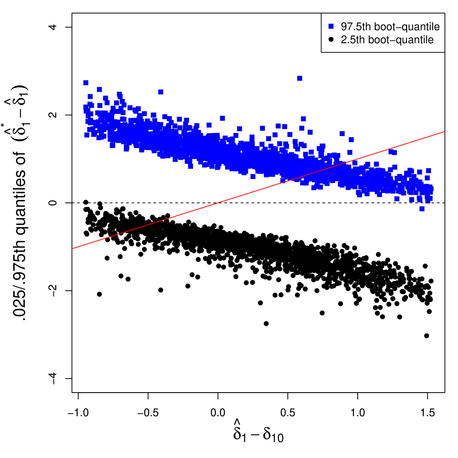
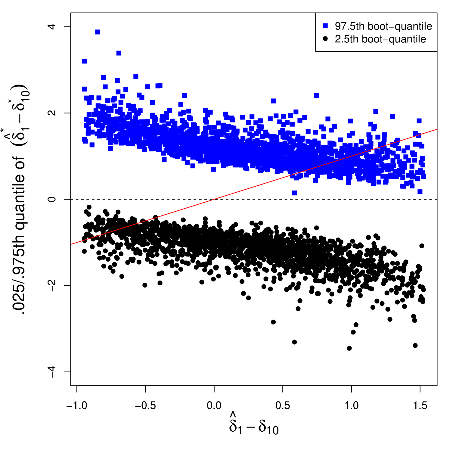
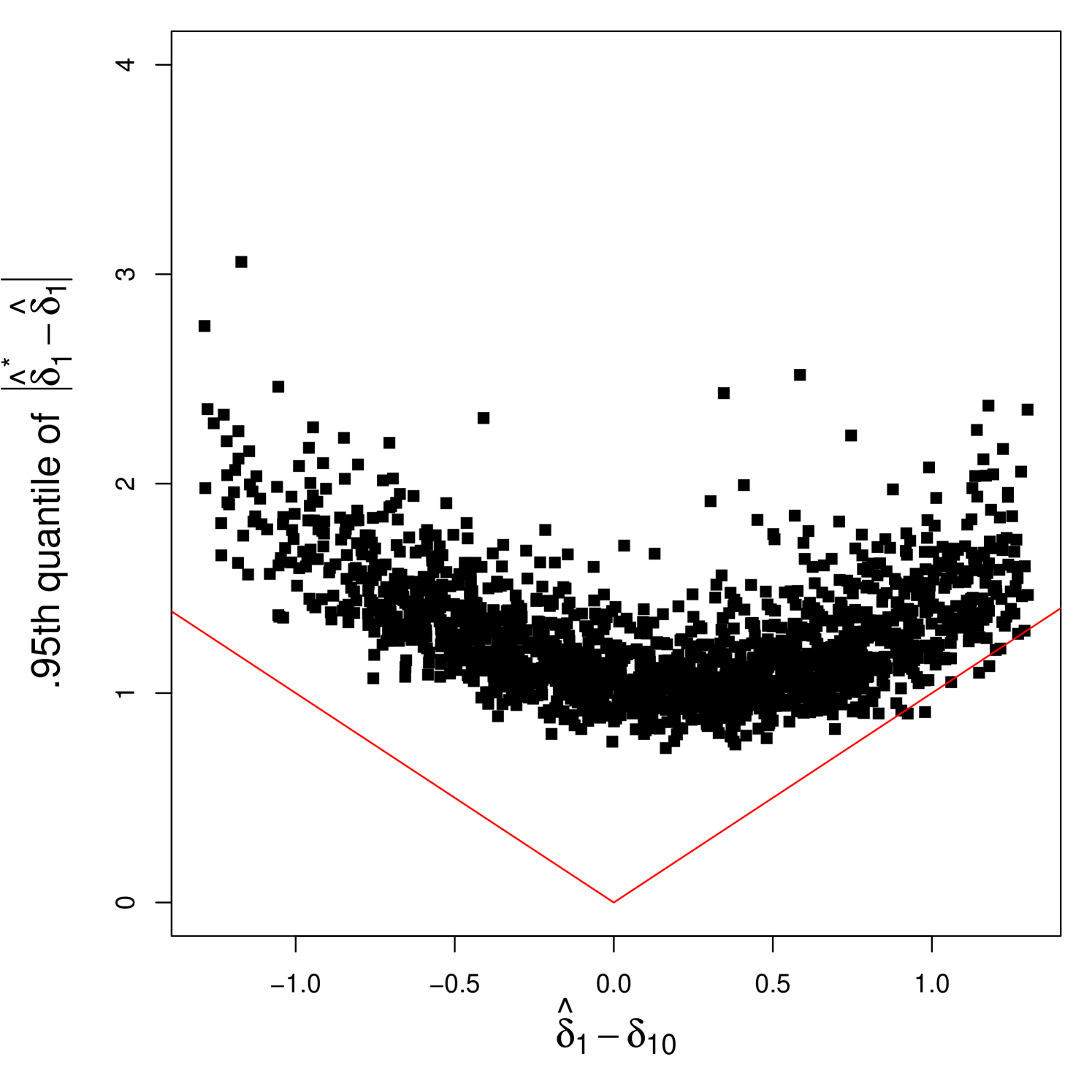
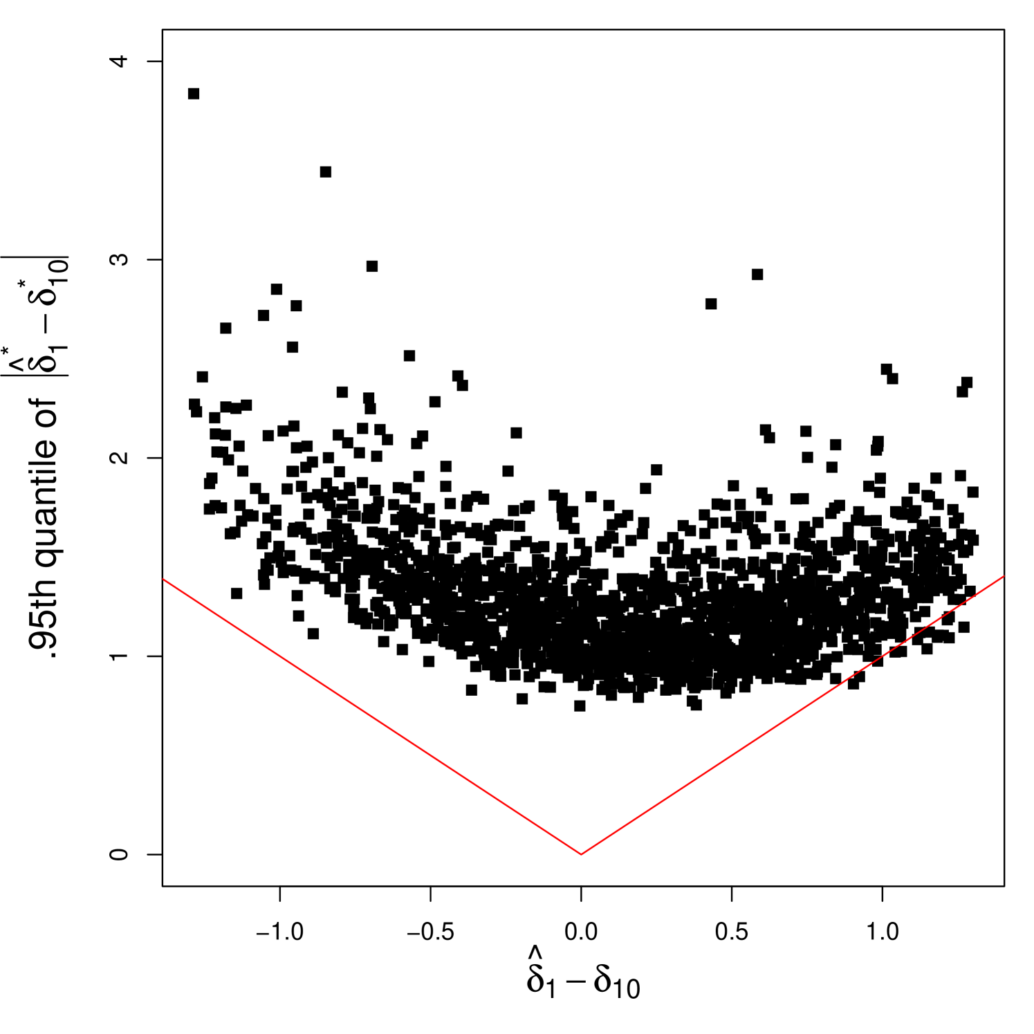
Notes: The figures plot the sample statistic (δ^1δ10)(\hat{\delta}_{1}-\delta_{10}) and the quantiles of the bootstrap test statistics relevant for confidence intervals for each simulated dataset from the continuous dgp where δ1+δ3γ=0\delta_{1}+\delta_{3}\gamma=0 with n=1600n=1600. Panels (a) and (b) show the 0.025 and 0.975 bootstrap quantiles of (δ^1δ^1)(\hat{\delta}_{1}^{*}-\hat{\delta}_{1}) (used for NP-B) and (δ^1δ10)(\hat{\delta}_{1}^{*}-\delta_{10}^{*}) (for R-B), respectively. Panels (c) and (d) show the 0.95 bootstrap quantiles of |δ^1δ^1||\hat{\delta}_{1}^{*}-\hat{\delta}_{1}| (for NP-B(S)) and |δ^1δ10||\hat{\delta}_{1}^{*}-\delta_{10}^{*}| (for R-B(S)), respectively. Red line represents a linear line with 45 degree in Panels (a) and (b), and the line y=|x|y=|x| in Panels (c) and (d). In Panels (a) and (b), the coverage probability is the frequency that the upper and lower bootstrap quantiles (dots) include the red line (45 degree line) between them. In Panels (c) and (d), the coverage probability is the frequency with which the bootstrap quantile (dot) lies above the red line.

Panels (a) and (b) show the 0.025 and 0.975 bootstrap quantiles of (δ^1δ^1)(\hat{\delta}_{1}^{*}-\hat{\delta}_{1}) (used for NP-B) and (δ^1δ10)(\hat{\delta}_{1}^{*}-\delta_{10}^{*}) (for R-B), respectively. The coverage probability is the frequency that the upper and lower bootstrap quantiles (dots) include the red line (45 degree line) between them. We observe that R-B method improves upon NP-B, as the distance between the two bootstrap quantiles tends to be wider. However, the improvement is not sufficiently large to resolve the undercoverage; see Table 3.

Note that the bootstrap quantiles (dots of each color) would be horizontally flat if they are asymptotically independent to the sample statistic. The nonparametric bootstrap CIs are asymptotically valid if

n(θ^θ^)d𝒵 in P when n(θ^θ0)𝑑𝒵,\sqrt{n}(\hat{\theta}^{*}-\hat{\theta})\xrightarrow{d^{*}}\mathcal{Z}^{*}\text{ in $P$ when }\sqrt{n}(\hat{\theta}-\theta_{0})\xrightarrow{d}\mathcal{Z},

where 𝒵\mathcal{Z}^{*} is an independent copy of 𝒵\mathcal{Z}. Therefore, the empirical 95% percentile of n(δ^1δ^1)\sqrt{n}(\hat{\delta}_{1}^{*}-\hat{\delta}_{1}) should be asymptotically independent to n(δ^1δ10)\sqrt{n}(\hat{\delta}_{1}-\delta_{10}) for the nonparametric bootstrap CI to be valid.

However, as shown in Panel (a), and the bootstrap quantiles are negatively correlated with the sample statistic. Specifically, the correlations between the sample statistic (δ^1δ10)(\hat{\delta}_{1}-\delta_{10}) and the 0.975 and 0.025 bootstrap quantiles from NP-B are -0.9037 and -0.8892, respectively. Our residual bootstrap (R-B) mitigates this issue. The bootstrap quantiles in Panel (b) appear flatter compared to those in Panel (a). The corresponding correlations from R-B are -0.7083 and -0.7003 for the 0.975 and 0.025 quantiles, respectively. While the correlations have decreased, they remain far from zero. Further investigation is warranted, although we leave this for future research.

Panels (c) and (d) show the 0.95 bootstrap quantiles of |δ^1δ^1||\hat{\delta}_{1}^{*}-\hat{\delta}_{1}| (for NP-B(S)) and |δ^1δ10||\hat{\delta}_{1}^{*}-\delta_{10}^{*}| (for R-B(S)), respectively. The coverage probability is the frequency of the dots that lie above the red line. Contrary to Panels (a) and (b), there is no rejection if δ^1δ10<0\hat{\delta}_{1}^{*}-\delta_{10}^{*}<0. Although this brings the coverage probabilities of both bootstraps closer to the nominal level, it is not desirable and misleading.

C.2 Weakly Endogenous Threshold Variable

We additionally report Monte Carlo results when the threshold variable is not weakly exogenous but weakly endogenous, that is, when the variable is predetermined. We consider the dgp same with the one in Section 5 with an exception that (12) is replaced by

(eituit)iidN((00),(1ρeuρeu1)),\begin{pmatrix}e_{it}\\ u_{it}\end{pmatrix}\overset{iid}{\sim}N\left(\begin{pmatrix}0\\ 0\end{pmatrix},\begin{pmatrix}1&\rho_{eu}\\ \rho_{eu}&1\end{pmatrix}\right), (C.2)

where ρeu=0.5\rho_{eu}=0.5. Other parameters such as θ=(β,δ,γ)\theta=(\beta^{\prime},\delta^{\prime},\gamma)^{\prime} and σ\sigma remain the same as in Section 5. Note that under (12), E[qisΔeit]=0E[q_{is}\Delta e_{it}]=0 if st1s\leq t-1. On the other hand, E[qisΔeit]=0E[q_{is}\Delta e_{it}]=0 if st2s\leq t-2 but E[qit1Δeit]0E[q_{it-1}\Delta e_{it}]\neq 0 under (C.2). Therefore, we need to exclude qit1q_{it-1} from the instrument such that zit=(yit2,,yi1,qit2,,qi1)z_{it}=(y_{it-2},\dots,y_{i1},q_{it-2},\dots,q_{i1})^{\prime}.

We consider the specifications where δ1+δ3γ=0,0.5,1\delta_{1}+\delta_{3}\gamma=0,0.5,1 and repeat Monte Carlo iterations 1,000 times. We report coverage rates of 95% CIs constructed by different bootstrap methods. Tables 9 and 10 show the coverage rates of the threshold location and the coefficients, respectively.

Table 9 shows that Grid-B achieves the most reasonable coverage rates, similar to the results in Table 1 in Section 5. Table 10 shows that both R-B and NP-B are subject to undercoverage for the coefficients, although R-B offers higher coverage rates than NP-B.

Table 9: Coverage rates of 95% CIs for the threshold location. Grid-B denotes the grid bootstrap CI defined by (7). NP-B and NP-B(S) denote the percentile and the symmetric percentile CIs by the standard nonparametric bootstrap defined by (13) and (14).
δ1+δ3γ\delta_{1}+\delta_{3}\gamma
n 0 0.5 1
400 0.990 0.983 0.975
Grid-B 800 0.986 0.983 0.965
1600 0.981 0.975 0.959
400 0.508 0.519 0.634
NP-B 800 0.443 0.496 0.612
1600 0.468 0.501 0.610
400 1.000 0.998 0.994
NP-B(S) 800 1.000 1.000 0.996
1600 1.000 0.999 0.999
Table 10: Coverage rates of 95% percentile CIs for the coefficients are shown. R-B denotes the percentile CIs by the residual bootstrap defined by (9). NP-B denotes the percentile CIs by the standard nonparametric bootstrap defined by (15).
R-B NP-B
δ1+δ3γ\delta_{1}+\delta_{3}\gamma n β2\beta_{2} β3\beta_{3} δ1\delta_{1} δ2\delta_{2} δ3\delta_{3} β2\beta_{2} β3\beta_{3} δ1\delta_{1} δ2\delta_{2} δ3\delta_{3}
400 0.753 0.739 0.781 0.796 0.765 0.726 0.658 0.636 0.706 0.691
0.0 800 0.795 0.729 0.783 0.786 0.756 0.764 0.629 0.640 0.709 0.669
1600 0.832 0.746 0.803 0.787 0.755 0.800 0.647 0.640 0.720 0.674
400 0.773 0.756 0.757 0.806 0.750 0.740 0.672 0.601 0.725 0.670
0.5 800 0.816 0.736 0.755 0.802 0.770 0.778 0.661 0.580 0.717 0.675
1600 0.835 0.746 0.776 0.791 0.770 0.811 0.660 0.605 0.720 0.660
400 0.805 0.777 0.743 0.822 0.754 0.765 0.712 0.618 0.731 0.701
1.0 800 0.829 0.770 0.725 0.798 0.742 0.784 0.685 0.582 0.727 0.683
1600 0.867 0.799 0.751 0.815 0.762 0.822 0.697 0.576 0.747 0.673

C.3 Coverage Rates by Asymptotic Confidence Intervals

We additionally report coverage rates of CIs based on the asymptotic method described in Seo and Shin, (2016). The dgp remains the same as in Section 5. Tables 11 and 12 show the results for the threshold and the coefficients, respectively.

Table 11 shows that the asymptotic method suffers undercoverage for all specifications we consider and does not improve as the sample size grows. This remains true even when δ1+δ3γ=1\delta_{1}+\delta_{3}\gamma=1, a case in which the model is discontinuous and the asymptotic CIs are theoretically valid, as shown in Seo and Shin, (2016). This especially highlights the desirability of our grid bootstrap method for inference of the threshold location which achieves good coverage rates in finite samples.

On the other hand, in Table 12, the coverage rates of the coefficients by the asymptotic method are much closer to the nominal level compared to those obtained from the nonparametric bootstrap or our residual bootstrap for both continuous and discontinuous models; see Table 3. We ask readers to be cautious, as it is unclear how the coverage rates of the asymptotic CIs behave when the true model is continuous, as explained in the last paragraph of Section 3.

Table 11: Coverage rates of 95% CIs for the threshold location by the asymptotic method described in Seo and Shin, (2016). The method is based on the asymptotic normality, which holds only when the true model is discontinuous.
δ1+δ3γ\delta_{1}+\delta_{3}\gamma
n 0 0.1 0.2 0.5 1
400 0.881 0.881 0.885 0.884 0.899
800 0.864 0.862 0.860 0.846 0.869
1600 0.837 0.836 0.837 0.836 0.864
Table 12: Coverage rates of 95% CIs for the coefficients by the asymptotic method described in Seo and Shin, (2016). The method is based on the asymptotic normality, which holds only when the true model is discontinuous.
δ1+δ3γ\delta_{1}+\delta_{3}\gamma n β2\beta_{2} β3\beta_{3} δ1\delta_{1} δ2\delta_{2} δ3\delta_{3}
400 0.950 0.923 0.951 0.916 0.970
0.0 800 0.956 0.921 0.952 0.921 0.973
1600 0.960 0.927 0.956 0.931 0.979
400 0.947 0.922 0.947 0.917 0.972
0.1 800 0.961 0.923 0.952 0.928 0.973
1600 0.960 0.929 0.956 0.933 0.983
400 0.942 0.919 0.947 0.915 0.974
0.2 800 0.959 0.926 0.952 0.926 0.971
1600 0.957 0.923 0.954 0.933 0.982
400 0.943 0.922 0.944 0.914 0.977
0.5 800 0.959 0.934 0.953 0.937 0.977
1600 0.953 0.934 0.953 0.930 0.983
400 0.949 0.937 0.950 0.925 0.987
1.0 800 0.958 0.952 0.952 0.945 0.985
1600 0.958 0.949 0.955 0.936 0.981

Appendix D Proofs of Theorems in Section 3 and Auxiliary Lemmas

Additional notations

We introduce additional notations as lemmas in this online appendix involve more empirical process theory. Suppose that (𝒳,𝒜)(\mathcal{X},\mathcal{A}) is a measurable space and ω1,ω2,\omega_{1},\omega_{2},... are i.i.d. random elements in (𝒳,𝒜)(\mathcal{X},\mathcal{A}) with probability law PP. For a point ω𝒳\omega\in\mathcal{X}, let δω\delta_{\omega} be a dirac measure at ω\omega444Although we already use δ\delta as the subvector of the parameter θ=(β,δ,γ)\theta=(\beta^{\prime},\delta^{\prime},\gamma)^{\prime}, we still use δ\delta to represent dirac measure as it is strong convention in the literature. We explicitly mention if δ\delta is used as dirac measure to avoid confusion.. The empirical measure of a sample ω1,,ωn\omega_{1},...,\omega_{n} is n=1ni=1nδωi\mathbb{P}_{n}=\frac{1}{n}\sum_{i=1}^{n}\delta_{\omega_{i}}, and the empirical process is 𝔾n=n(nP)\mathbb{G}_{n}=\sqrt{n}(\mathbb{P}_{n}-P). Let \mathcal{F} be a functional class, elements of which are measurable functions from 𝒳\mathcal{X} to \mathbb{R}. We call a function F:𝒳F:\mathcal{X}\rightarrow\mathbb{R} an envelope of \mathcal{F} if |f|F|f|\leq F for all ff\in\mathcal{F}. For a stochastic process 𝔾\mathbb{G} and a functional class \mathcal{F}, define 𝔾:=supf|𝔾f|\|\mathbb{G}\|_{\mathcal{F}}:=\sup_{f\in\mathcal{F}}|\mathbb{G}f|.

D.1 Proof of Theorem 3.

D.1.1 Continuous Model.

When γ=γ0\gamma=\gamma_{0}.

Note that the constrained estimator α^(γ0)=argminαAQ^n(α,γ0)\hat{\alpha}(\gamma_{0})=\arg\min_{\alpha\in A}\hat{Q}_{n}(\alpha,\gamma_{0}) is n\sqrt{n}-consistent to α0\alpha_{0}, which is identical to the convergence rate of α^\hat{\alpha}, since the problem becomes a standard linear dynamic panel estimation. Let a=n(αα0)a=\sqrt{n}(\alpha-\alpha_{0}) and b=n1/4(γγ0)b=n^{1/4}(\gamma-\gamma_{0}). The distance test statistic can be rewritten as follows:

𝒟n(γ0)\displaystyle\mathcal{D}_{n}(\gamma_{0}) =\displaystyle= infa𝕊n(a,0)infa,b𝕊n(a,b)+op(1)\displaystyle\inf_{a}\mathbb{S}_{n}(a,0)-\inf_{a,b}\mathbb{S}_{n}(a,b)+o_{p}(1)
𝑑\displaystyle\xrightarrow{d} infa𝕊(a,0)infa,b𝕊(a,b)\displaystyle\inf_{a}\mathbb{S}(a,0)-\inf_{a,b}\mathbb{S}(a,b)
=\displaystyle= mina(M0ae)Ω1(M0ae)mina,b2(M0a+Hb2e)Ω1(M0a+Hb2e),\displaystyle\min_{a}(M_{0}a-e)^{\prime}\Omega^{-1}(M_{0}a-e)-\min_{a,b^{2}}(M_{0}a+Hb^{2}-e)^{\prime}\Omega^{-1}(M_{0}a+Hb^{2}-e),

where we apply the CMT. Lee et al., (2011) showed that the difference between the constrained and unconstrained infima is a continuous operator on (𝕂)\ell^{\infty}(\mathbb{K}).

Note that mina(M0ae)Ω1(M0ae)=e(Ω1Ω1M0(M0Ω1M0)1M0Ω1)e\min_{a}(M_{0}a-e)^{\prime}\Omega^{-1}(M_{0}a-e)=e^{\prime}(\Omega^{-1}-\Omega^{-1}M_{0}(M_{0}^{\prime}\Omega^{-1}M_{0})^{-1}M_{0}^{\prime}\Omega^{-1})e, while

mina,b2(M0a+Hb2e)Ω1(M0a+Hb2e)\displaystyle\min_{a,b^{2}}(M_{0}a+Hb^{2}-e)^{\prime}\Omega^{-1}(M_{0}a+Hb^{2}-e)
=(M0a0+Hb02e)Ω1(M0a0+Hb02e)\displaystyle=(M_{0}a_{0}+Hb_{0}^{2}-e)^{\prime}\Omega^{-1}(M_{0}a_{0}+Hb_{0}^{2}-e)
=(M0Ω1M0a0+M0Ω1Hb02)(M0Ω1M0)1(M0Ω1M0a0+M0Ω1Hb02)\displaystyle=(M_{0}^{\prime}\Omega^{-1}M_{0}a_{0}+M_{0}^{\prime}\Omega^{-1}Hb_{0}^{2})^{\prime}(M_{0}^{\prime}\Omega^{-1}M_{0})^{-1}(M_{0}^{\prime}\Omega^{-1}M_{0}a_{0}+M_{0}^{\prime}\Omega^{-1}Hb_{0}^{2})
+b02HΩ1/2(IPΩ1/2M0)Ω1/2Hb022eΩ1M0(M0Ω1M0)1(M0Ω1M0a0+M0Ω1Hb02)\displaystyle\quad+b_{0}^{2}H^{\prime}\Omega^{-1/2}(I-P_{\Omega^{-1/2}M_{0}})\Omega^{-1/2}Hb_{0}^{2}-2e^{\prime}\Omega^{-1}M_{0}(M_{0}^{\prime}\Omega^{-1}M_{0})^{-1}(M_{0}^{\prime}\Omega^{-1}M_{0}a_{0}+M_{0}^{\prime}\Omega^{-1}Hb_{0}^{2})
2eΩ1/2(IPΩ1/2M0)Ω1/2Hb02+eΩ1e,\displaystyle\quad-2e^{\prime}\Omega^{-1/2}(I-P_{\Omega^{-1/2}M_{0}})\Omega^{-1/2}Hb_{0}^{2}+e^{\prime}\Omega^{-1}e,

where (a0,b02)(a_{0},b_{0}^{2}) is the argmin, whose formula is derived in the proof of Theorem 2. By plugging in one of the first order conditions, M0Ω1M0a0+M0Ω1Hb02=M0Ω1eM_{0}^{\prime}\Omega^{-1}M_{0}a_{0}+M_{0}^{\prime}\Omega^{-1}Hb_{0}^{2}=M_{0}^{\prime}\Omega^{-1}e, and the formula for b0b_{0}, we can get

mina,b2(M0a+Hb2e)Ω1(M0a+Hb2e)\displaystyle\min_{a,b^{2}}(M_{0}a+Hb^{2}-e)^{\prime}\Omega^{-1}(M_{0}a+Hb^{2}-e)
={eΩ1M0(M0Ω1M0)1M0Ω1eeΞH(HΞH)1HΞe+eΩ1eif HΞe0eΩ1M0(M0Ω1M0)1M0Ω1e+eΩ1eelse.\displaystyle\quad=\begin{cases}-e^{\prime}\Omega^{-1}M_{0}(M_{0}^{\prime}\Omega^{-1}M_{0})^{-1}M_{0}^{\prime}\Omega^{-1}e-e^{\prime}\Xi H(H^{\prime}\Xi H)^{-1}H^{\prime}\Xi e+e^{\prime}\Omega^{-1}e&\text{if }H^{\prime}\Xi e\geq 0\\ -e^{\prime}\Omega^{-1}M_{0}(M_{0}^{\prime}\Omega^{-1}M_{0})^{-1}M_{0}^{\prime}\Omega^{-1}e+e^{\prime}\Omega^{-1}e&\text{else}.\end{cases}

Therefore, the limit distribution of the test statistic is identical to

{eΞH(HΞH)1HΞeif HΞe00else.\begin{cases}e^{\prime}\Xi H(H^{\prime}\Xi H)^{-1}H^{\prime}\Xi e&\text{if }H^{\prime}\Xi e\geq 0\\ 0&\text{else}.\end{cases}

Note that eΞH(HΞH)1HΞeχ12e^{\prime}\Xi H(H^{\prime}\Xi H)^{-1}H^{\prime}\Xi e\sim\chi^{2}_{1} as HΞeN(0,HΞΩΞH)H^{\prime}\Xi e\sim N(0,H^{\prime}\Xi\Omega\Xi H), and HΞΩΞH=HΞHH^{\prime}\Xi\Omega\Xi H=H^{\prime}\Xi H.

When γγ0\gamma\neq\gamma_{0}.

We show that 𝒟n(γ)\mathcal{D}_{n}(\gamma) diverges to infinity in probability. There is a constant C1(0,+)C_{1}\in(0,+\infty) such that infαAg0(α,γ)C1\inf_{\alpha\in A}\|g_{0}(\alpha,\gamma)\|\geq C_{1}. This is because g0(θ)g_{0}(\theta) is zero if and only if θ=θ0\theta=\theta_{0}, by G and Theorem 1, and continuous on Θ\Theta, by D, while the restricted parameter set {θ=(β,δ,γ)Θ:γ=c}\{\theta=(\beta^{\prime},\delta^{\prime},\gamma)^{\prime}\in\Theta:\gamma=c\} is closed for all cΓc\in\Gamma. 𝒢={g(ωi,θ):θΘ}\mathcal{G}=\{g(\omega_{i},\theta):\theta\in\Theta\} is shown to satisfy the uniform entropy condition in the proof of Lemma D.3, and hence supθΘg¯n(θ)g0(θ)=op(1)\sup_{\theta\in\Theta}\|\bar{g}_{n}(\theta)-g_{0}(\theta)\|=o_{p}(1) by Glivenko-Cantelli theorem. By triangle inequality, C1g0(α^(γ),γ)g¯n(α^(γ),γ)+op(1)C_{1}\leq\|g_{0}(\hat{\alpha}(\gamma),\gamma)\|\leq\|\bar{g}_{n}(\hat{\alpha}(\gamma),\gamma)\|+o_{p}(1). Meanwhile, g¯n(θ^)=Op(n1/2)\|\bar{g}_{n}(\hat{\theta})\|=O_{p}(n^{-1/2}) because g¯n(θ^)g¯n(θ0)=Op(n1/2)\|\bar{g}_{n}(\hat{\theta})\|\leq\|\bar{g}_{n}(\theta_{0})\|=O_{p}(n^{-1/2}). Therefore, there exists C2(0,+)C_{2}\in(0,+\infty) such that Q^n(α^(γ),γ)Q^n(θ^)C2+Op(n1)\hat{Q}_{n}(\hat{\alpha}(\gamma),\gamma)-\hat{Q}_{n}(\hat{\theta})\geq C_{2}+O_{p}(n^{-1}), which implies that P(𝒟n(γ)>M)=P(Q^n(α^(γ),γ)Q^n(θ^)>M/n)1P(\mathcal{D}_{n}(\gamma)>M)=P(\hat{Q}_{n}(\hat{\alpha}(\gamma),\gamma)-\hat{Q}_{n}(\hat{\theta})>M/n)\rightarrow 1 for any M<M<\infty.

D.1.2 Discontinuous Model.

When γ=γ0\gamma=\gamma_{0}.

As in the proof for the continuous model, we apply the CMT to the test statistic. Let a=n(αα0)a=\sqrt{n}(\alpha-\alpha_{0}) and b=n(γγ0)b=\sqrt{n}(\gamma-\gamma_{0}). First, we will show that when the model is discontinuous and Assumptions G, D, and LJ are true, 𝕊n(a,b)𝕊J(a,b)=(M0a+Gbe)Ω1(M0a+Gbe)\mathbb{S}_{n}(a,b)\rightsquigarrow\mathbb{S}_{J}(a,b)=(M_{0}a+Gb-e)^{\prime}\Omega^{-1}(M_{0}a+Gb-e) in (𝕂)\ell^{\infty}(\mathbb{K}) for any compact 𝕂2p+2\mathbb{K}\subset\mathbb{R}^{2p+2}. Note that

ng¯n(α0+an,γ0+bn)=\displaystyle\sqrt{n}\bar{g}_{n}(\alpha_{0}+\tfrac{a}{\sqrt{n}},\gamma_{0}+\tfrac{b}{\sqrt{n}})= n(1ni=1nzit0Δϵit01ni=1nziTΔϵiT)(1ni=1nzit0Δxit01ni=1nziTΔxiT)a1\displaystyle\sqrt{n}\begin{pmatrix}\frac{1}{n}\sum_{i=1}^{n}z_{it_{0}}\Delta\epsilon_{it_{0}}\\ \vdots\\ \frac{1}{n}\sum_{i=1}^{n}z_{iT}\Delta\epsilon_{iT}\end{pmatrix}-\begin{pmatrix}\tfrac{1}{n}\sum_{i=1}^{n}z_{it_{0}}\Delta x_{it_{0}}^{\prime}\\ \vdots\\ \tfrac{1}{n}\sum_{i=1}^{n}z_{iT}\Delta x_{iT}^{\prime}\end{pmatrix}a_{1} (D.1)
(1ni=1nzit01it0(γ0+bn)Xit01ni=1nziT1iT(γ0+bn)XiT)a2\displaystyle-\begin{pmatrix}\tfrac{1}{n}\sum_{i=1}^{n}z_{it_{0}}1_{it_{0}}(\gamma_{0}+\tfrac{b}{\sqrt{n}})^{\prime}X_{it_{0}}\\ \vdots\\ \tfrac{1}{n}\sum_{i=1}^{n}z_{iT}1_{iT}(\gamma_{0}+\tfrac{b}{\sqrt{n}})^{\prime}X_{iT}\end{pmatrix}a_{2} (D.2)
+n(1ni=1nzit0(1it0(γ0)1it0(γ0+bn))Xit01ni=1nziT(1iT(γ0)1iT(γ0+bn))XiT)δ0.\displaystyle+\sqrt{n}\begin{pmatrix}\tfrac{1}{n}\sum_{i=1}^{n}z_{it_{0}}(1_{it_{0}}(\gamma_{0})^{\prime}-1_{it_{0}}(\gamma_{0}+\tfrac{b}{\sqrt{n}})^{\prime})X_{it_{0}}\\ \vdots\\ \tfrac{1}{n}\sum_{i=1}^{n}z_{iT}(1_{iT}(\gamma_{0})^{\prime}-1_{iT}(\gamma_{0}+\tfrac{b}{\sqrt{n}})^{\prime})X_{iT}\end{pmatrix}\delta_{0}. (D.3)

The terms in the first two lines of the right hand side (D.1) and (D.2) converge in distribution to (M0ae)(M_{0}a-e) uniformly with respect to b[K,K]b\in[-K,K]. Since supb:|b|Kng¯n(α0,γ0+bn)g¯n(α0,γ0)g0(α0,γ0+bn)+g0(α0,γ0)=op(1)\sup_{b:|b|\leq K}\sqrt{n}\|\bar{g}_{n}(\alpha_{0},\gamma_{0}+\frac{b}{\sqrt{n}})-\bar{g}_{n}(\alpha_{0},\gamma_{0})-g_{0}(\alpha_{0},\gamma_{0}+\frac{b}{\sqrt{n}})+g_{0}(\alpha_{0},\gamma_{0})\|=o_{p}(1) by Lemma D.3,

n(1ni=1nzit0(1it0(γ0)1it0(γ0+bn))Xit0δ01ni=1nziT(1iT(γ0)1iT(γ0+bn))XiTδ0)(E[zit0(1it0(γ0)1it0(γ0+bn))Xit0δ0]E[ziT(1iT(γ0)1iT(γ0+bn))XiTδ0])\sqrt{n}\left\|\begin{pmatrix}\tfrac{1}{n}\sum_{i=1}^{n}z_{it_{0}}(1_{it_{0}}(\gamma_{0})^{\prime}-1_{it_{0}}(\gamma_{0}+\tfrac{b}{\sqrt{n}})^{\prime})X_{it_{0}}\delta_{0}\\ \vdots\\ \tfrac{1}{n}\sum_{i=1}^{n}z_{iT}(1_{iT}(\gamma_{0})^{\prime}-1_{iT}(\gamma_{0}+\tfrac{b}{\sqrt{n}})^{\prime})X_{iT}\delta_{0}\end{pmatrix}-\begin{pmatrix}E[z_{it_{0}}(1_{it_{0}}(\gamma_{0})^{\prime}-1_{it_{0}}(\gamma_{0}+\tfrac{b}{\sqrt{n}})^{\prime})X_{it_{0}}\delta_{0}]\\ \vdots\\ E[z_{iT}(1_{iT}(\gamma_{0})^{\prime}-1_{iT}(\gamma_{0}+\tfrac{b}{\sqrt{n}})^{\prime})X_{iT}\delta_{0}]\end{pmatrix}\right\|

converges in probability to zero uniformly with respect to b[K,K]b\in[-K,K]. Suppose b>0b>0. The result for b<0b<0 is similar. By application of Talyor expansion,

nE[zit(1,xit)δ01{γ0+bnqit>γ0}]Et[zit(1,xit)δ0|γ0]ft(γ0)b,\sqrt{n}E[z_{it}(1,x_{it}^{\prime})\delta_{0}1\{\gamma_{0}+\tfrac{b}{\sqrt{n}}\geq q_{it}>\gamma_{0}\}]\rightarrow E_{t}[z_{it}(1,x_{it}^{\prime})\delta_{0}|\gamma_{0}]f_{t}(\gamma_{0})b,

uniformly with respect to b[K,K]b\in[-K,K], and similar limit result can be derived for nE[zit((1,xit1)δ01{γ0+bnqit1>γ0}]\sqrt{n}E[z_{it}((1,x_{it-1}^{\prime})\delta_{0}1\{\gamma_{0}+\tfrac{b}{\sqrt{n}}\geq q_{it-1}>\gamma_{0}\}]. Hence, we can derive that the term (D.3) converges in probability to GbGb uniformly with respect to b[K,K]b\in[-K,K].

By the CMT, the test statistic converges in distribution to

mina(M0ae)Ω1(M0ae)mina,b(M0a+Gbe)Ω1(M0a+Gbe).\min_{a}(M_{0}a-e)^{\prime}\Omega^{-1}(M_{0}a-e)-\min_{a,b}(M_{0}a+Gb-e)^{\prime}\Omega^{-1}(M_{0}a+Gb-e).

Note that mina(M0ae)Ω1(M0ae)=e(Ω1Ω1M0(M0Ω1M0)1M0Ω1)e\min_{a}(M_{0}a-e)^{\prime}\Omega^{-1}(M_{0}a-e)=e^{\prime}(\Omega^{-1}-\Omega^{-1}M_{0}(M_{0}^{\prime}\Omega^{-1}M_{0})^{-1}M_{0}^{\prime}\Omega^{-1})e, and mina,b(M0a+Gbe)Ω1(M0a+Gbe)=e(Ω1Ω1D1(D1Ω1D1)1D1Ω1)e\min_{a,b}(M_{0}a+Gb-e)^{\prime}\Omega^{-1}(M_{0}a+Gb-e)=e^{\prime}(\Omega^{-1}-\Omega^{-1}D_{1}(D_{1}^{\prime}\Omega^{-1}D_{1})^{-1}D_{1}^{\prime}\Omega^{-1})e. Therefore, the limit distribution of the test statistic is identical to the distribution of

eΩ1/2[Ω1/2D1(D1Ω1D1)1D1Ω1/2Ω1/2M0(M0Ω1M0)1M0Ω1/2]Ω1/2e.e^{\prime}\Omega^{-1/2}[\Omega^{-1/2}D_{1}(D_{1}^{\prime}\Omega^{-1}D_{1})^{-1}D_{1}^{\prime}\Omega^{-1/2}-\Omega^{-1/2}M_{0}(M_{0}^{\prime}\Omega^{-1}M_{0})^{-1}M_{0}^{\prime}\Omega^{-1/2}]\Omega^{-1/2}e.

The matrix Ω1/2D1(D1Ω1D1)1D1Ω1/2Ω1/2M0(M0Ω1M0)1M0Ω1/2\Omega^{-1/2}D_{1}(D_{1}^{\prime}\Omega^{-1}D_{1})^{-1}D_{1}^{\prime}\Omega^{-1/2}-\Omega^{-1/2}M_{0}(M_{0}^{\prime}\Omega^{-1}M_{0})^{-1}M_{0}^{\prime}\Omega^{-1/2} is idempotent since the column space of Ω1/2M0\Omega^{-1/2}M_{0} lies in the column space of Ω1/2D1\Omega^{-1/2}D_{1}. The rank of the matrix is 1. Since Ω1/2eN(0,I)\Omega^{-1/2}e\sim N(0,I), the chi-square distribution with 1 degree of freedom is the limit distribution.

When γγ0\gamma\neq\gamma_{0}.

The proof showing that 𝒟n(γ)\mathcal{D}_{n}(\gamma) diverges when γγ0\gamma\neq\gamma_{0} for the discontinuous model is identical to the proof written for the continuous model.

D.2 Proof of Theorem 4.

Under the null hypothesis.

Define a map TT such that T(ψ)=(β,γδ3,0,,0,δ3,γ)2p+2T(\psi)=(\beta^{\prime},-\gamma\delta_{3},0,...,0,\delta_{3},\gamma)^{\prime}\in\mathbb{R}^{2p+2} if ψ=(β,δ3,γ)p+2\psi=(\beta^{\prime},\delta_{3},\gamma)^{\prime}\in\mathbb{R}^{p+2}. Let ψ0=(β0,δ30,γ0)\psi_{0}=(\beta_{0}^{\prime},\delta_{30},\gamma_{0})^{\prime}. Note that

gi(T(ψ))=(zit0{Δyit0Δxit0β[(qit0γ)1{qit0>γ}(qit01γ)1{qit01>γ}]δ3}ziT{ΔyiTΔxiTβ[(qiTγ)1{qiT>γ}(qiT1γ)1{qiT1>γ}]δ3}).g_{i}(T(\psi))=\begin{pmatrix}z_{it_{0}}\{\Delta y_{it_{0}}-\Delta x_{it_{0}}^{\prime}\beta-[(q_{it_{0}}-\gamma)1_{\{q_{it_{0}}>\gamma\}}-(q_{it_{0}-1}-\gamma)1_{\{q_{it_{0}-1}>\gamma\}}]\delta_{3}\}\\ \vdots\\ z_{iT}\{\Delta y_{iT}-\Delta x_{iT}^{\prime}\beta-[(q_{iT}-\gamma)1_{\{q_{iT}>\gamma\}}-(q_{iT-1}-\gamma)1_{\{q_{iT-1}>\gamma\}}]\delta_{3}\}\end{pmatrix}.

The first-order derivative of g0(T(ψ))g_{0}(T(\psi)) with respect to ψ\psi is

Dψ=E[zit0Δxit0,zit0[(qit0γ0)1{qit0>γ0}(qit01γ0)1{qit01>γ0}],zit0[1{qit0>γ0}1{qit01>γ0}]δ30ziTΔxiT,ziT[(qiTγ0)1{qiT>γ0}(qiT1γ0)1{qiT1>γ0}],ziT[1{qiT>γ0}1{qiT1>γ0}]δ30].D_{\psi}=\\ E\begin{bmatrix}-z_{it_{0}}\Delta x_{it_{0}}^{\prime},&-z_{it_{0}}[(q_{it_{0}}-\gamma_{0})1_{\{q_{it_{0}}>\gamma_{0}\}}-(q_{it_{0}-1}-\gamma_{0})1_{\{q_{it_{0}-1}>\gamma_{0}\}}],&z_{it_{0}}[1_{\{q_{it_{0}}>\gamma_{0}\}}-1_{\{q_{it_{0}-1}>\gamma_{0}\}}]\delta_{30}\\ \vdots&\vdots&\vdots\\ -z_{iT}\Delta x_{iT}^{\prime},&-z_{iT}[(q_{iT}-\gamma_{0})1_{\{q_{iT}>\gamma_{0}\}}-(q_{iT-1}-\gamma_{0})1_{\{q_{iT-1}>\gamma_{0}\}}],&z_{iT}[1_{\{q_{iT}>\gamma_{0}\}}-1_{\{q_{iT-1}>\gamma_{0}\}}]\delta_{30}\end{bmatrix}.

DψD_{\psi} is a matrix that is identical to a binding of the columns of M10M_{10} and N20N_{20}. If ψ^=argminψQ^n(T(ψ))\hat{\psi}=\arg\min_{\psi}\hat{Q}_{n}(T(\psi)), then n(ψ^ψ0)𝑑N(0,(DψΩDψ)1)\sqrt{n}(\hat{\psi}-\psi_{0})\xrightarrow{d}N(0,(D_{\psi}^{\prime}\Omega D_{\psi})^{-1}) (see Kim et al., (2019)). The continuity test statistic 𝒯n=n(Q^n(θ~)Q^n(θ^))\mathcal{T}_{n}=n(\hat{Q}_{n}(\tilde{\theta})-\hat{Q}_{n}(\hat{\theta})) can be rewritten as

n(Q^n(T(ψ^))Q^n(θ^))=n(min(θ,ψ):θ=θ0(Q^n(T(ψ))Q^n(θ))min(θ,ψ):ψ=ψ0(Q^n(T(ψ))+Q^n(θ))).n(\hat{Q}_{n}(T(\hat{\psi}))-\hat{Q}_{n}(\hat{\theta}))=n\left(\min_{(\theta^{\prime},\psi^{\prime})^{\prime}:\theta=\theta_{0}}(\hat{Q}_{n}(T(\psi))-\hat{Q}_{n}(\theta))-\min_{(\theta^{\prime},\psi^{\prime})^{\prime}:\psi=\psi_{0}}(-\hat{Q}_{n}(T(\psi))+\hat{Q}_{n}(\theta))\right).

Reparametrize such that a=n(αα0)a=\sqrt{n}(\alpha-\alpha_{0}), b=n1/4(γγ0)b=n^{1/4}(\gamma-\gamma_{0}), and r=n(ψψ0)r=\sqrt{n}(\psi-\psi_{0}). Define a centered criterion by

𝕄n(a,b,r)=n(Q^n(T(ψ0+rn))Q^n(α0+an,γ0+bn14)).\mathbb{M}_{n}(a,b,r)=n(\hat{Q}_{n}(T(\psi_{0}+\tfrac{r}{\sqrt{n}}))-\hat{Q}_{n}(\alpha_{0}+\tfrac{a}{\sqrt{n}},\gamma_{0}+\tfrac{b}{n^{\frac{1}{4}}})).

We will show that 𝕄n\mathbb{M}_{n} weakly converges to a process 𝕄\mathbb{M} in (𝕂)\ell^{\infty}(\mathbb{K}) for every compact 𝕂3p+4\mathbb{K}\subset\mathbb{R}^{3p+4}. Then, by the CMT, the continuity test statistic converges in distribution to

min(a,b,r):(a,b)=0𝕄(a,b,r)min(a,b,r):r=0(𝕄(a,b,r)).\min_{(a^{\prime},b,r^{\prime})^{\prime}:(a^{\prime},b)^{\prime}=0}\mathbb{M}(a,b,r)-\min_{(a^{\prime},b,r^{\prime})^{\prime}:r=0}(-\mathbb{M}(a,b,r)).

In the proof of Theorem 2, it is shown that ng¯n(α0+an,γ0+bn14)(M0a+Hb2e)\sqrt{n}\bar{g}_{n}(\alpha_{0}+\tfrac{a}{\sqrt{n}},\gamma_{0}+\tfrac{b}{n^{\frac{1}{4}}})\rightsquigarrow(M_{0}a+Hb^{2}-e) and

nQ^n(α0+an,γ0+bn14)(M0a+Hb2e)Ω1(M0a+Hb2e).n\hat{Q}_{n}(\alpha_{0}+\tfrac{a}{\sqrt{n}},\gamma_{0}+\tfrac{b}{n^{\frac{1}{4}}})\rightsquigarrow(M_{0}a+Hb^{2}-e)^{\prime}\Omega^{-1}(M_{0}a+Hb^{2}-e).

Let r1=n(ββ0)r_{1}=\sqrt{n}(\beta-\beta_{0}), r2=(r21,r22)r_{2}=(r_{21},r_{22})^{\prime}, r21=n(δ3δ30)r_{21}=\sqrt{n}(\delta_{3}-\delta_{30}), and r22=n(γγ0)r_{22}=\sqrt{n}(\gamma-\gamma_{0}). Then,

ng¯n(T(ψ0+rn))\displaystyle\sqrt{n}\bar{g}_{n}(T(\psi_{0}+\tfrac{r}{\sqrt{n}}))
=(1ni=1nzit0Δϵit01ni=1nziTΔϵiT)(1ni=1nzit0Δxit01ni=1nziTΔxiT)r1\displaystyle=\begin{pmatrix}\frac{1}{\sqrt{n}}\sum_{i=1}^{n}z_{it_{0}}\Delta\epsilon_{it_{0}}\\ \vdots\\ \frac{1}{\sqrt{n}}\sum_{i=1}^{n}z_{iT}\Delta\epsilon_{iT}\end{pmatrix}-\begin{pmatrix}\frac{1}{n}\sum_{i=1}^{n}z_{it_{0}}\Delta x_{it_{0}}\\ \vdots\\ \frac{1}{n}\sum_{i=1}^{n}z_{iT}\Delta x_{iT}\end{pmatrix}r_{1}
(1ni=1nzit0[(qit0γ0r22n)1{qit0>γ0+r22n}(qit01γ0r22n)1{qit01>γ0+r22n}]1ni=1nziT[(qiTγ0r22n)1{qiT>γ0+r22n}(qiT1γ0r22n)1{qiT1>γ0+r22n}])r21\displaystyle-\begin{pmatrix}\frac{1}{n}\sum_{i=1}^{n}z_{it_{0}}[(q_{it_{0}}-\gamma_{0}-\frac{r_{22}}{\sqrt{n}})1\{q_{it_{0}}>\gamma_{0}+\frac{r_{22}}{\sqrt{n}}\}-(q_{it_{0}-1}-\gamma_{0}-\frac{r_{22}}{\sqrt{n}})1\{q_{it_{0}-1}>\gamma_{0}+\frac{r_{22}}{\sqrt{n}}\}]\\ \vdots\\ \frac{1}{n}\sum_{i=1}^{n}z_{iT}[(q_{iT}-\gamma_{0}-\frac{r_{22}}{\sqrt{n}})1\{q_{iT}>\gamma_{0}+\frac{r_{22}}{\sqrt{n}}\}-(q_{iT-1}-\gamma_{0}-\frac{r_{22}}{\sqrt{n}})1\{q_{iT-1}>\gamma_{0}+\frac{r_{22}}{\sqrt{n}}\}]\end{pmatrix}r_{21}
+n{(1ni=1nzit0[(qit0γ0)1{qit0>γ0}(qit0γ0r22n)1{qit0>γ0+r22n}]1ni=1nziT[(qiTγ0)1{qiT>γ0}(qiTγ0r22n)1{qiT>γ0+r22n}])\displaystyle+\sqrt{n}\left\{\begin{pmatrix}\frac{1}{n}\sum_{i=1}^{n}z_{it_{0}}[(q_{it_{0}}-\gamma_{0})1\{q_{it_{0}}>\gamma_{0}\}-(q_{it_{0}}-\gamma_{0}-\frac{r_{22}}{\sqrt{n}})1\{q_{it_{0}}>\gamma_{0}+\frac{r_{22}}{\sqrt{n}}\}]\\ \vdots\\ \frac{1}{n}\sum_{i=1}^{n}z_{iT}[(q_{iT}-\gamma_{0})1\{q_{iT}>\gamma_{0}\}-(q_{iT}-\gamma_{0}-\frac{r_{22}}{\sqrt{n}})1\{q_{iT}>\gamma_{0}+\frac{r_{22}}{\sqrt{n}}\}]\end{pmatrix}\right.
(1ni=1nzit0[(qit01γ0)1{qit01>γ0}(qit01γ0r22n)1{qit01>γ0+r22n}]1ni=1nziT[(qiT1γ0)1{qiT1>γ0}(qiT1γ0r22n)1{qiT1>γ0+r22n}])}δ30.\displaystyle\left.\qquad-\begin{pmatrix}\frac{1}{n}\sum_{i=1}^{n}z_{it_{0}}[(q_{it_{0}-1}-\gamma_{0})1\{q_{it_{0}-1}>\gamma_{0}\}-(q_{it_{0}-1}-\gamma_{0}-\frac{r_{22}}{\sqrt{n}})1\{q_{it_{0}-1}>\gamma_{0}+\frac{r_{22}}{\sqrt{n}}\}]\\ \vdots\\ \frac{1}{n}\sum_{i=1}^{n}z_{iT}[(q_{iT-1}-\gamma_{0})1\{q_{iT-1}>\gamma_{0}\}-(q_{iT-1}-\gamma_{0}-\frac{r_{22}}{\sqrt{n}})1\{q_{iT-1}>\gamma_{0}+\frac{r_{22}}{\sqrt{n}}\}]\end{pmatrix}\right\}\delta_{30}.

By the CLT and LLN,

(1ni=1nzit0Δϵit01ni=1nziTΔϵiT)(1ni=1nzit0Δxit01ni=1nziTΔxiT)r1𝑑(M10r1e).\begin{pmatrix}\frac{1}{\sqrt{n}}\sum_{i=1}^{n}z_{it_{0}}\Delta\epsilon_{it_{0}}\\ \vdots\\ \frac{1}{\sqrt{n}}\sum_{i=1}^{n}z_{iT}\Delta\epsilon_{iT}\end{pmatrix}-\begin{pmatrix}\frac{1}{n}\sum_{i=1}^{n}z_{it_{0}}\Delta x_{it_{0}}\\ \vdots\\ \frac{1}{n}\sum_{i=1}^{n}z_{iT}\Delta x_{iT}\end{pmatrix}r_{1}\xrightarrow{d}(M_{10}r_{1}-e).

By the ULLN (application of Lemma D.2) and continuity of κE[zit(1,qit)1{qit>γ0+κ}]\kappa\mapsto E[z_{it}(1,q_{it})1\{q_{it}>\gamma_{0}+\kappa\}] and κE[zit(1,qit1)1{qit1>γ0+κ}]\kappa\mapsto E[z_{it}(1,q_{it-1})1\{q_{it-1}>\gamma_{0}+\kappa\}] at κ=0\kappa=0,

(1ni=1nzit0[(qit0γ0r22n)1{qit0>γ0+r22n}(qit01γ0r22n)1{qit01>γ0+r22n}]1ni=1nziT[(qiTγ0r22n)1{qiT>γ0+r22n}(qiT1γ0r22n)1{qiT1>γ0+r22n}])r21𝑝(Ezit0[(qit0γ0)1{qit0>γ0}(qit01γ0)1{qit01>γ0}]EziT[(qiTγ0)1{qiT>γ0}(qiT1γ0)1{qiT1>γ0}])r21\begin{pmatrix}\frac{1}{n}\sum_{i=1}^{n}z_{it_{0}}[(q_{it_{0}}-\gamma_{0}-\frac{r_{22}}{\sqrt{n}})1\{q_{it_{0}}>\gamma_{0}+\frac{r_{22}}{\sqrt{n}}\}-(q_{it_{0}-1}-\gamma_{0}-\frac{r_{22}}{\sqrt{n}})1\{q_{it_{0}-1}>\gamma_{0}+\frac{r_{22}}{\sqrt{n}}\}]\\ \vdots\\ \frac{1}{n}\sum_{i=1}^{n}z_{iT}[(q_{iT}-\gamma_{0}-\frac{r_{22}}{\sqrt{n}})1\{q_{iT}>\gamma_{0}+\frac{r_{22}}{\sqrt{n}}\}-(q_{iT-1}-\gamma_{0}-\frac{r_{22}}{\sqrt{n}})1\{q_{iT-1}>\gamma_{0}+\frac{r_{22}}{\sqrt{n}}\}]\end{pmatrix}r_{21}\\ \xrightarrow{p}\begin{pmatrix}Ez_{it_{0}}[(q_{it_{0}}-\gamma_{0})1\{q_{it_{0}}>\gamma_{0}\}-(q_{it_{0}-1}-\gamma_{0})1\{q_{it_{0}-1}>\gamma_{0}\}]\\ \vdots\\ Ez_{iT}[(q_{iT}-\gamma_{0})1\{q_{iT}>\gamma_{0}\}-(q_{iT-1}-\gamma_{0})1\{q_{iT-1}>\gamma_{0}\}]\end{pmatrix}r_{21}

uniformly with respect to r22[K,K]r_{22}\in[-K,K]. Finally,

n{(1ni=1nzit0[(qit0γ0)1{qit0>γ0}(qit0γ0r22n)1{qit0>γ0+r22n}]1ni=1nziT[(qiTγ0)1{qiT>γ0}(qiTγ0r22n)1{qiT>γ0+r22n}])(1ni=1nzit0[(qit01γ0)1{qit01>γ0}(qit01γ0r22n)1{qit01>γ0+r22n}]1ni=1nziT[(qiT1γ0)1{qiT1>γ0}(qiT1γ0r22n)1{qiT1>γ0+r22n}])}𝑝(Ezit0[1{qit0>γ0}1{qit01>γ0}]EziT[1{qiT>γ0}1{qiT1>γ0}])r22\sqrt{n}\left\{\begin{pmatrix}\frac{1}{n}\sum_{i=1}^{n}z_{it_{0}}[(q_{it_{0}}-\gamma_{0})1\{q_{it_{0}}>\gamma_{0}\}-(q_{it_{0}}-\gamma_{0}-\frac{r_{22}}{\sqrt{n}})1\{q_{it_{0}}>\gamma_{0}+\frac{r_{22}}{\sqrt{n}}\}]\\ \vdots\\ \frac{1}{n}\sum_{i=1}^{n}z_{iT}[(q_{iT}-\gamma_{0})1\{q_{iT}>\gamma_{0}\}-(q_{iT}-\gamma_{0}-\frac{r_{22}}{\sqrt{n}})1\{q_{iT}>\gamma_{0}+\frac{r_{22}}{\sqrt{n}}\}]\end{pmatrix}\right.\\ \left.\qquad-\begin{pmatrix}\frac{1}{n}\sum_{i=1}^{n}z_{it_{0}}[(q_{it_{0}-1}-\gamma_{0})1\{q_{it_{0}-1}>\gamma_{0}\}-(q_{it_{0}-1}-\gamma_{0}-\frac{r_{22}}{\sqrt{n}})1\{q_{it_{0}-1}>\gamma_{0}+\frac{r_{22}}{\sqrt{n}}\}]\\ \vdots\\ \frac{1}{n}\sum_{i=1}^{n}z_{iT}[(q_{iT-1}-\gamma_{0})1\{q_{iT-1}>\gamma_{0}\}-(q_{iT-1}-\gamma_{0}-\frac{r_{22}}{\sqrt{n}})1\{q_{iT-1}>\gamma_{0}+\frac{r_{22}}{\sqrt{n}}\}]\end{pmatrix}\right\}\\ \xrightarrow{p}\begin{pmatrix}Ez_{it_{0}}[1\{q_{it_{0}}>\gamma_{0}\}-1\{q_{it_{0}-1}>\gamma_{0}\}]\\ \vdots\\ Ez_{iT}[1\{q_{iT}>\gamma_{0}\}-1\{q_{iT-1}>\gamma_{0}\}]\end{pmatrix}r_{22}

uniformly with respect to r22[K,K]r_{22}\in[-K,K]. Suppose that r22>0r_{22}>0. The case for r22<0r_{22}<0 follows similarly. The last uniform convergence holds because Lemma D.3 yields ng¯n(T(β0,δ30,γ0+r22n))g¯n(T(β0,δ30,γ0))g0(T(β0,δ30,γ0+r22n))+g0(T(β0,δ30,γ0))=op(1)\sqrt{n}\|\bar{g}_{n}(T(\beta_{0},\delta_{30},\gamma_{0}+\frac{r_{22}}{\sqrt{n}}))-\bar{g}_{n}(T(\beta_{0},\delta_{30},\gamma_{0}))-g_{0}(T(\beta_{0},\delta_{30},\gamma_{0}+\frac{r_{22}}{\sqrt{n}}))+g_{0}(T(\beta_{0},\delta_{30},\gamma_{0}))\|=o_{p}(1) uniformly with respect to r22[K,K]r_{22}\in[-K,K] and the following application of Taylor expansion:

nE[zit((qitγ0)1{qit>γ0}(qitγ0r22n)1{qit>γ0+r22n})]\displaystyle\sqrt{n}E[z_{it}((q_{it}-\gamma_{0})1\{q_{it}>\gamma_{0}\}-(q_{it}-\gamma_{0}-\frac{r_{22}}{\sqrt{n}})1\{q_{it}>\gamma_{0}+\frac{r_{22}}{\sqrt{n}}\})]
=nE[zit(qitγ0)1{γ0+r22nqit>γ0}]+r22E[zit1{qit>γ0+r22n}]\displaystyle=\sqrt{n}E[z_{it}(q_{it}-\gamma_{0})1\{\gamma_{0}+\frac{r_{22}}{\sqrt{n}}\geq q_{it}>\gamma_{0}\}]+r_{22}E[z_{it}1\{q_{it}>\gamma_{0}+\frac{r_{22}}{\sqrt{n}}\}]
Et[zit(qitγ0)|γ0]ft(γ0)r22+E[zit1{qit>γ0}]r22=E[zit1{qit>γ0}]r22\displaystyle\rightarrow E_{t}[z_{it}(q_{it}-\gamma_{0})|\gamma_{0}]f_{t}(\gamma_{0})r_{22}+E[z_{it}1\{q_{it}>\gamma_{0}\}]r_{22}=E[z_{it}1\{q_{it}>\gamma_{0}\}]r_{22}

uniformly with respect to r22[K,K]r_{22}\in[-K,K] as nn\rightarrow\infty.

In conclusion, ng¯n(T(ψ0+rn))(Dψre)\sqrt{n}\bar{g}_{n}(T(\psi_{0}+\tfrac{r}{\sqrt{n}}))\rightsquigarrow(D_{\psi}r-e), and

𝕄(a,b,r)\displaystyle\mathbb{M}(a,b,r) =(Dψre)Ω1(Dψre)(M0a+Hb2e)Ω1(M0a+Hb2e)\displaystyle=(D_{\psi}r-e)^{\prime}\Omega^{-1}(D_{\psi}r-e)-(M_{0}a+Hb^{2}-e)^{\prime}\Omega^{-1}(M_{0}a+Hb^{2}-e)
=(M10r1+N20r2e)Ω1(M10r1+N20r2e)\displaystyle=(M_{10}r_{1}+N_{20}r_{2}-e)^{\prime}\Omega^{-1}(M_{10}r_{1}+N_{20}r_{2}-e)
(M10a1+M20a2+Hb2e)Ω1(M10a1+M20a2+Hb2e),\displaystyle\qquad-(M_{10}a_{1}+M_{20}a_{2}+Hb^{2}-e)^{\prime}\Omega^{-1}(M_{10}a_{1}+M_{20}a_{2}+Hb^{2}-e),

where a1=n(ββ0)a_{1}=\sqrt{n}(\beta-\beta_{0}) and a2=n(δδ0)a_{2}=\sqrt{n}(\delta-\delta_{0}). By applying the CMT, the continuity test statistic converges in distribution to

minr(M10r1+N20r2e)Ω1(M10r1+N20r2e)\displaystyle\min_{r}(M_{10}r_{1}+N_{20}r_{2}-e)^{\prime}\Omega^{-1}(M_{10}r_{1}+N_{20}r_{2}-e)
mina,b2(M10a1+M20a2+Hb2e)Ω1(M10a1+M20a2+Hb2e).\displaystyle\qquad-\min_{a,b^{2}}(M_{10}a_{1}+M_{20}a_{2}+Hb^{2}-e)^{\prime}\Omega^{-1}(M_{10}a_{1}+M_{20}a_{2}+Hb^{2}-e).

By similar computations to the proof of Theorem 3,

minr1,r2(M10r1+N20r2e)Ω1(M10r1+N20r2e)\displaystyle\min_{r_{1},r_{2}}(M_{10}r_{1}+N_{20}r_{2}-e)^{\prime}\Omega^{-1}(M_{10}r_{1}+N_{20}r_{2}-e)
=eΩ1eeΩ1M10(M10Ω1M10)1M10Ω1eeΞ1N20(N20Ξ1N20)1N20Ξ1e,\displaystyle\quad=e^{\prime}\Omega^{-1}e-e^{\prime}\Omega^{-1}M_{10}(M_{10}^{\prime}\Omega^{-1}M_{10})^{-1}M_{10}^{\prime}\Omega^{-1}e-e^{\prime}\Xi_{1}N_{20}(N_{20}^{\prime}\Xi_{1}N_{20})^{-1}N_{20}^{\prime}\Xi_{1}e,
mina1,a2,b2(M10a1+M20a2+Hb2e)Ω1(M10a1+M20a2+Hb2e)\displaystyle\min_{a_{1},a_{2},b^{2}}(M_{10}a_{1}+M_{20}a_{2}+Hb^{2}-e)^{\prime}\Omega^{-1}(M_{10}a_{1}+M_{20}a_{2}+Hb^{2}-e)
={eΩ1M10(M10Ω1M10)1M10Ω1eeΞ1M20(M20Ξ1M20)1M20Ξ1eeΞ12H(HΞ12H)1HΞ12e+eΩ1eif HΞ12e0eΩ1M10(M10Ω1M10)1M10Ω1eeΞ1M20(M20Ξ1M20)1M20Ξ1e+eΩ1e else\displaystyle\quad=\begin{cases}\begin{array}[]{l}-e^{\prime}\Omega^{-1}M_{10}(M_{10}^{\prime}\Omega^{-1}M_{10})^{-1}M_{10}^{\prime}\Omega^{-1}e-e^{\prime}\Xi_{1}M_{20}(M_{20}^{\prime}\Xi_{1}M_{20})^{-1}M_{20}^{\prime}\Xi_{1}e\\ -e^{\prime}\Xi_{12}H(H^{\prime}\Xi_{12}H)^{-1}H^{\prime}\Xi_{12}e+e^{\prime}\Omega^{-1}e\end{array}&\hskip-25.60747pt\text{if }H^{\prime}\Xi_{12}e\geq 0\\ &\\ -e^{\prime}\Omega^{-1}M_{10}(M_{10}^{\prime}\Omega^{-1}M_{10})^{-1}M_{10}^{\prime}\Omega^{-1}e-e^{\prime}\Xi_{1}M_{20}(M_{20}^{\prime}\Xi_{1}M_{20})^{-1}M_{20}^{\prime}\Xi_{1}e+e^{\prime}\Omega^{-1}e&\text{ else}\end{cases}

where Ξ1=Ω1/2(IΩ1/2M10(M10Ω1M10)1M10Ω1/2)Ω1/2\Xi_{1}=\Omega^{-1/2}(I-\Omega^{-1/2}M_{10}(M_{10}^{\prime}\Omega^{-1}M_{10})^{-1}M_{10}^{\prime}\Omega^{-1/2})\Omega^{-1/2} and Ξ12=Ξ11/2(IΞ11/2M20(M20Ξ1M20)1M20Ξ11/2)Ξ11/2\Xi_{12}=\Xi_{1}^{1/2}(I-\Xi_{1}^{1/2}M_{20}(M_{20}^{\prime}\Xi_{1}M_{20})^{-1}M_{20}^{\prime}\Xi_{1}^{1/2})\Xi_{1}^{1/2}. As Ξ1ΩΞ1=Ξ1\Xi_{1}\Omega\Xi_{1}=\Xi_{1}, we can derive Ξ12ΩΞ12=(Ξ1Ξ1M20(M20Ξ1M20)1M20Ξ1)Ω(Ξ1Ξ1M20(M20Ξ1M20)1M20Ξ1)=Ξ1Ξ1M20(M20Ξ1M20)1M20Ξ1=Ξ12\Xi_{12}\Omega\Xi_{12}=(\Xi_{1}-\Xi_{1}M_{20}(M_{20}^{\prime}\Xi_{1}M_{20})^{-1}M_{20}^{\prime}\Xi_{1})\Omega(\Xi_{1}-\Xi_{1}M_{20}(M_{20}^{\prime}\Xi_{1}M_{20})^{-1}M_{20}^{\prime}\Xi_{1})=\Xi_{1}-\Xi_{1}M_{20}(M_{20}^{\prime}\Xi_{1}M_{20})^{-1}M_{20}^{\prime}\Xi_{1}=\Xi_{12}, and hence eΞ12H(HΞ12H)1HΞ12eχ12e^{\prime}\Xi_{12}H(H^{\prime}\Xi_{12}H)^{-1}H^{\prime}\Xi_{12}e\sim\chi^{2}_{1}. Since E[HΞ12eeΞ1M20]E[H^{\prime}\Xi_{12}ee^{\prime}\Xi_{1}M_{20}] is zero, (eΞ1M20(M20Ξ1M20)1M20Ξ1e,eΞ1N20(N20Ξ1N20)1N20Ξ1e)(e^{\prime}\Xi_{1}M_{20}(M_{20}^{\prime}\Xi_{1}M_{20})^{-1}M_{20}^{\prime}\Xi_{1}e,e^{\prime}\Xi_{1}N_{20}(N_{20}^{\prime}\Xi_{1}N_{20})^{-1}N_{20}^{\prime}\Xi_{1}e) is independent to eΞ12H(HΞ12H)1HΞ12ee^{\prime}\Xi_{12}H(H^{\prime}\Xi_{12}H)^{-1}H^{\prime}\Xi_{12}e.

Under the alternative hypothesis.

There is a constant C1(0,+)C_{1}\in(0,+\infty) such that infθΘ:δ1+δ3γ=0,δ2=0p1g0(θ)C1\inf_{\theta\in\Theta:\delta_{1}+\delta_{3}\gamma=0,\delta_{2}=0_{p-1}}\|g_{0}(\theta)\|\geq C_{1}. This is because g0(θ)g_{0}(\theta) is zero if and only if θ=θ0\theta=\theta_{0}, by G and Theorem 1, and continuous on Θ\Theta, by D, while the restricted parameter set {θ=(β,δ,γ):δ2=0p1,δ1+δ3γ=0}\{\theta=(\beta^{\prime},\delta^{\prime},\gamma)^{\prime}:\delta_{2}=0_{p-1},\delta_{1}+\delta_{3}\gamma=0\} is closed. 𝒢={g(ωi,θ):θΘ}\mathcal{G}=\{g(\omega_{i},\theta):\theta\in\Theta\} is shown to satisfy the uniform entropy condition in the proof of Lemma D.3, and hence supθΘg¯n(θ)g0(θ)=op(1)\sup_{\theta\in\Theta}\|\bar{g}_{n}(\theta)-g_{0}(\theta)\|=o_{p}(1) by Glivenko-Cantelli theorem. By triangle inequality, C1g0(θ~)g¯n(θ~)+op(1)C_{1}\leq\|g_{0}(\tilde{\theta})\|\leq\|\bar{g}_{n}(\tilde{\theta})\|+o_{p}(1). Recall that θ~\tilde{\theta} is the continuity-restricted estimator. Meanwhile, g¯n(θ^)=Op(n1/2)\|\bar{g}_{n}(\hat{\theta})\|=O_{p}(n^{-1/2}) because g¯n(θ^)g¯n(θ0)=Op(n1/2)\|\bar{g}_{n}(\hat{\theta})\|\leq\|\bar{g}_{n}(\theta_{0})\|=O_{p}(n^{-1/2}). Therefore, there exists C2(0,+)C_{2}\in(0,+\infty) such that Q^n(θ~)Q^n(θ^)C2+Op(n1)\hat{Q}_{n}(\tilde{\theta})-\hat{Q}_{n}(\hat{\theta})\geq C_{2}+O_{p}(n^{-1}), which implies that P(nm𝒯n>M)=P(Q^n(θ~)Q^n(θ^)>M/(n1m))1P(n^{-m}\mathcal{T}_{n}>M)=P(\hat{Q}_{n}(\tilde{\theta})-\hat{Q}_{n}(\hat{\theta})>M/(n^{1-m}))\rightarrow 1, for any m[0,1)m\in[0,1) and M<M<\infty.

D.3 Auxiliary Lemmas

Lemma D.1.

Suppose that the true model is continuous and Assumptions G, D, and LK are true. For any η>0\eta>0, there is a neighborhood 𝒪\mathcal{O} of θ0\theta_{0} such that the population moment function g0(θ)g_{0}(\theta) satisfies

limnsupθ𝒪ng0(θ)D2(αα0,(γγ0)2)1+n(αα0,(γγ0)2)<η.\lim_{n\rightarrow\infty}\sup_{\theta\in\mathcal{O}}\frac{\sqrt{n}\|g_{0}(\theta)-D_{2}\left(\alpha^{\prime}-\alpha_{0}^{\prime},(\gamma-\gamma_{0})^{2}\right)^{\prime}\|}{1+\sqrt{n}\|\left(\alpha^{\prime}-\alpha_{0}^{\prime},(\gamma-\gamma_{0})^{2}\right)^{\prime}\|}<\eta.
Proof.

Recall that GG, whose formula is (5), is the first-order derivative of g0(θ)g_{0}(\theta) with respect to γ\gamma at θ=θ0\theta=\theta_{0}, and HH, whose formula is (6), is a half of the second-order derivative. GG can be obtained by applying the Leibniz rule as follows:

ddγE[zit(1,xit)δ01{qit>γ}]|γ=γ0\displaystyle\left.\frac{d}{d\gamma}E[-z_{it}(1,x_{it}^{\prime})\delta_{0}1\{q_{it}>\gamma\}]\right|_{\gamma=\gamma_{0}} =ddγγEt[zit(1,xit)δ0|q]ft(q)dq|γ=γ0\displaystyle=\left.\frac{d}{d\gamma}\int_{\gamma}^{\infty}-E_{t}[z_{it}(1,x_{it}^{\prime})\delta_{0}|q]f_{t}(q)dq\right|_{\gamma=\gamma_{0}}
=Et[zit(1,xit)δ0|γ0]ft(γ0).\displaystyle=E_{t}[z_{it}(1,x_{it}^{\prime})\delta_{0}|\gamma_{0}]f_{t}(\gamma_{0}).

Similarly, we can get

ddγE[zit(1,xit1)δ01{qit1>γ}]|γ=γ0=Et1[zit(1,xit1)δ0|γ0]ft1(γ0).\left.\frac{d}{d\gamma}E[z_{it}(1,x_{it-1}^{\prime})\delta_{0}1\{q_{it-1}>\gamma\}]\right|_{\gamma=\gamma_{0}}=-E_{t-1}[z_{it}(1,x_{it-1}^{\prime})\delta_{0}|\gamma_{0}]f_{t-1}(\gamma_{0}).

This implies the formula (5) for GG. HH can also be obtained by the Leibniz rule as follows:

ddγEt[zit(1,xit)δ0|γ]ft(γ)|γ=γ0\displaystyle\left.\frac{d}{d\gamma}E_{t}[z_{it}(1,x_{it}^{\prime})\delta_{0}|\gamma]f_{t}(\gamma)\right|_{\gamma=\gamma_{0}} =ddγEt[zit(δ10+δ30γ)|γ]ft(γ)|γ=γ0\displaystyle=\left.\frac{d}{d\gamma}E_{t}[z_{it}(\delta_{10}+\delta_{30}\gamma)|\gamma]f_{t}(\gamma)\right|_{\gamma=\gamma_{0}}
=ddγ(δ10+δ30γ)Et[zit|γ]ft(γ)|γ=γ0\displaystyle=\left.\frac{d}{d\gamma}(\delta_{10}+\delta_{30}\gamma)\cdot E_{t}[z_{it}|\gamma]f_{t}(\gamma)\right|_{\gamma=\gamma_{0}}
=δ30Et[zit|γ0]ft(γ0)+(δ10+δ30γ0)ddγEt[zit|γ]ft(γ)|γ=γ0\displaystyle=\delta_{30}E_{t}[{z_{it}}|\gamma_{0}]f_{t}(\gamma_{0})+(\delta_{10}+\delta_{30}\gamma_{0})\left.\frac{d}{d\gamma}E_{t}[z_{it}|\gamma]f_{t}(\gamma)\right|_{\gamma=\gamma_{0}}
=δ30Et[zit|γ0]ft(γ0).\displaystyle=\delta_{30}E_{t}[{z_{it}}|\gamma_{0}]f_{t}(\gamma_{0}).

Similarly, we can get

ddγ{Et1[zit(1,xit1)δ0|γ]ft1(γ)}|γ=γ0=δ30Et1[zit|γ0]ft1(γ0).\left.\frac{d}{d\gamma}\{-E_{t-1}[z_{it}(1,x_{it-1}^{\prime})\delta_{0}|\gamma]f_{t-1}(\gamma)\}\right|_{\gamma=\gamma_{0}}=-\delta_{30}E_{t-1}[{z_{it}}|\gamma_{0}]f_{t-1}(\gamma_{0}).

This implies the formula (6) for HH.

The population moment can be expressed as,

g0(α,γ)=M0(γ)(αα0)+H(γγ0)2+o((γγ0)2).g_{0}(\alpha,\gamma)=M_{0}(\gamma)(\alpha-\alpha_{0})+H(\gamma-\gamma_{0})^{2}+o((\gamma-\gamma_{0})^{2}).

Define M0,G=[0k×pM_G]k×(2p+1)M_{0,G}=\left[\begin{array}[]{c;{2pt/2pt}c}0_{k\times p}&M_{G}\end{array}\right]\in\mathbb{R}^{k\times(2p+1)} where

MG=[Et0[zit0(1,xit0)|γ0]ft0(γ0)Et01[zit0(1,xit01)|γ0]ft01(γ0)ET[ziT(1,xiT)|γ0]fT(γ0)ET1[ziT(1,xiT1)|γ0]fT1(γ0)]k×(p+1).M_{G}=\begin{bmatrix}E_{t_{0}}[z_{it_{0}}(1,x_{it_{0}}^{\prime})|\gamma_{0}]f_{t_{0}}(\gamma_{0})-E_{t_{0}-1}[z_{it_{0}}(1,x_{it_{0}-1}^{\prime})|\gamma_{0}]f_{t_{0}-1}(\gamma_{0})\\ \vdots\\ E_{T}[z_{iT}(1,x_{iT}^{\prime})|\gamma_{0}]f_{T}(\gamma_{0})-E_{T-1}[z_{iT}(1,x_{iT-1}^{\prime})|\gamma_{0}]f_{T-1}(\gamma_{0})\end{bmatrix}\in\mathbb{R}^{k\times(p+1)}.

The polynomial expansion M0(γ)=M0+M0,G(γγ0)+o(|γγ0|)M_{0}(\gamma)=M_{0}+M_{0,G}(\gamma-\gamma_{0})+o(|\gamma-\gamma_{0}|) implies

g0(α,γ)=M0(αα0)+H(γγ0)2+o(αα0+(γγ0)2).g_{0}(\alpha,\gamma)=M_{0}(\alpha-\alpha_{0})+H(\gamma-\gamma_{0})^{2}+o(\|\alpha-\alpha_{0}\|+(\gamma-\gamma_{0})^{2}).

Thus, ng0(θ)D2(αα0,(γγ0)2)=o(n(αα0+(γγ0)2))\sqrt{n}\|g_{0}(\theta)-D_{2}\left(\alpha^{\prime}-\alpha_{0}^{\prime},(\gamma-\gamma_{0})^{2}\right)^{\prime}\|=o(\sqrt{n}(\|\alpha-\alpha_{0}\|+(\gamma-\gamma_{0})^{2})), which completes the proof. ∎

Lemma D.2.

If G is true, then

supγΓM¯n(γ)M0(γ)𝑝0.\sup_{\gamma\in\Gamma}\|\bar{M}_{n}(\gamma)-M_{0}(\gamma)\|\xrightarrow{p}0.
Proof.

We show that the classes {zit(1,xit)1{qit>γ}:γΓ}\{z_{it}(1,x_{it}^{\prime})1\{q_{it}>\gamma\}:\gamma\in\Gamma\} and {zit(1,xit1)1{qit1>γ}:γΓ}\{z_{it}(1,x_{it-1}^{\prime})1\{q_{it-1}>\gamma\}:\gamma\in\Gamma\} are P-Glivenko-Cantelli. We focus on the former class since the verification for the latter class is exactly identical. Let ωi={(zit,yit,xit,ϵit)t=1T}\omega_{i}=\{(z_{it},y_{it},x_{it},\epsilon_{it})_{t=1}^{T}\} be a random element in a measurable space (𝒳,𝒜)(\mathcal{X},\mathcal{A}). A collection of measurable index functions 𝒢index={1{qit>γ}:γΓ}\mathcal{G}_{index}=\{1\{q_{it}>\gamma\}:\gamma\in\Gamma\} on 𝒳\mathcal{X} is a VC class with a VC index 2. If mijm_{ij} is the (i,j)(i,j)th element of zit(1,xit)z_{it}(1,x_{it}^{\prime}), then 𝒢indexmij={gindexmij:gindex𝒢index}\mathcal{G}_{index}\cdot m_{ij}=\{g_{index}\cdot m_{ij}:g_{index}\in\mathcal{G}_{index}\} is also a VC class as discussed by Lemma 2.6.18 in van der Vaart and Wellner, (1996). The envelope for 𝒢indexmij\mathcal{G}_{index}\cdot m_{ij} would be |mij||m_{ij}| since an index function is always bounded by 1. The expectation of the envelope is bounded since Ezit(1,xit)Ezit2E(1,xit)2<E\|z_{it}(1,x_{it}^{\prime})\|\leq\sqrt{E\|z_{it}\|^{2}E\|(1,x_{it}^{\prime})^{\prime}\|^{2}}<\infty. In conclusion, 𝒢indexmij\mathcal{G}_{index}\cdot m_{ij} is a PP-Glivenko-Cantelli for each (i,j)(i,j), and thus the ULLN for {zit(1,xit)1{qit>γ}:γΓ}\{z_{it}(1,x_{it}^{\prime})1\{q_{it}>\gamma\}:\gamma\in\Gamma\} holds. ∎

Lemma D.3.

Let G hold. If hn0h_{n}\rightarrow 0, then

supθ1θ2<hnng¯n(θ1)g¯n(θ2)g0(θ1)+g0(θ2)=op(1).\sup_{\|\theta_{1}-\theta_{2}\|<h_{n}}\sqrt{n}\|\bar{g}_{n}(\theta_{1})-\bar{g}_{n}(\theta_{2})-g_{0}(\theta_{1})+g_{0}(\theta_{2})\|=o_{p}(1).
Proof.

Let ωi={(zit,yit,xit,ϵit)t=1T}\omega_{i}=\{(z_{it},y_{it},x_{it},\epsilon_{it})_{t=1}^{T}\} be a random element in a measurable space (𝒳,𝒜)(\mathcal{X},\mathcal{A}), and PP is the probability measure for ωi\omega_{i}. Define a functional class 𝒢={g(ωi,θ):θΘ}\mathcal{G}=\{g(\omega_{i},\theta):\theta\in\Theta\} on 𝒳\mathcal{X} such that

g(ωi,θ)\displaystyle g(\omega_{i},\theta) =(gt0(ωi,θ),,gT(ωi,θ)),\displaystyle=(g_{t_{0}}(\omega_{i},\theta)^{\prime},...,g_{T}(\omega_{i},\theta)^{\prime})^{\prime}, (D.4)
gt(ωi,θ)\displaystyle g_{t}(\omega_{i},\theta) =zitΔyitzitΔxitβzit1it(γ)Xitδ\displaystyle=z_{it}\Delta y_{it}-z_{it}\Delta x_{it}^{\prime}\beta-z_{it}1_{it}(\gamma)^{\prime}X_{it}\delta
=zitΔϵitzitΔxit(ββ0)zit1it(γ)Xit(δδ0)+zit(1it(γ0)1it(γ))Xitδ0.\displaystyle=z_{it}\Delta\epsilon_{it}-z_{it}\Delta x_{it}^{\prime}(\beta-\beta_{0})-z_{it}1_{it}(\gamma)^{\prime}X_{it}(\delta-\delta_{0})+z_{it}(1_{it}(\gamma_{0})^{\prime}-1_{it}(\gamma)^{\prime})X_{it}\delta_{0}.

and 𝒢h={g(ωi,θ1)g(ωi,θ2):θ1θ2<h,θ1,θ2Θ}\mathcal{G}_{h}=\{g(\omega_{i},\theta_{1})-g(\omega_{i},\theta_{2}):\|\theta_{1}-\theta_{2}\|<h,\theta_{1},\theta_{2}\in\Theta\}. We need to show that P(𝔾n𝒢h>x)0P(\|\mathbb{G}_{n}\|_{\mathcal{G}_{h}}>x)\rightarrow 0 if h0h\rightarrow 0 as nn\rightarrow\infty, which is the asymptotic equicontinuity. To show the asymptotic equicontinuity, it is sufficient to show that each element of 𝒢\mathcal{G} is P-Donsker, e.g., 2.3.11 Lemma and its corollary in van der Vaart and Wellner, (1996), which is implied by the uniform entropy condtion:

0supQlogN(εGQ,2,𝒢,L2(Q))dε<,\int_{0}^{\infty}\sup_{Q}\sqrt{\log N(\varepsilon\|G\|_{Q,2},\mathcal{G},L_{2}(Q))}d\varepsilon<\infty,

where supremum is taken over all probability measures QQ on (𝒳,𝒜)(\mathcal{X},\mathcal{A}) such that QG2<QG^{2}<\infty, and GG is an envelope for 𝒢\mathcal{G}. For more details, see section 2.1 in van der Vaart and Wellner, (1996). As we only need to consider each scalar element of 𝒢\mathcal{G}, it is sufficient to consider the following functional class

𝒢~(t)={zitΔϵitzitΔxitβ¯zit1it(γ1)Xitδ1+zit1it(γ2)Xitδ2:β¯K,δ1K,δ2K,γ1,γ2Γ},\widetilde{\mathcal{G}}^{(t)}=\{z_{it}\Delta\epsilon_{it}-z_{it}\Delta x_{it}\bar{\beta}-z_{it}1_{it}(\gamma_{1})^{\prime}X_{it}\delta_{1}+z_{it}1_{it}(\gamma_{2})^{\prime}X_{it}\delta_{2}\\ :\|\bar{\beta}\|\leq K,\|\delta_{1}\|\leq K,\|\delta_{2}\|\leq K,\gamma_{1},\gamma_{2}\in\Gamma\},

where K<K<\infty is a constant such that θK/2\|\theta\|\leq K/2 if θΘ\theta\in\Theta. Assume that zitz_{it} is a scalar without losing of generality. Note that gt(ωi,θ)=zit(ΔyitΔxitβ1it(γ)Xitδ)=zitΔϵitzitΔxit(ββ0n)zit1it(γ)Xitδ+zit1it(γ0)Xitδ0g_{t}(\omega_{i},\theta)=z_{it}(\Delta y_{it}-\Delta x_{it}^{\prime}\beta-1_{it}(\gamma)^{\prime}X_{it}\delta)=z_{it}\Delta\epsilon_{it}-z_{it}\Delta x_{it}(\beta-\beta_{0n})-z_{it}1_{it}(\gamma)^{\prime}X_{it}\delta+z_{it}1_{it}(\gamma_{0})^{\prime}X_{it}\delta_{0} is an element of 𝒢~(t)\widetilde{\mathcal{G}}^{(t)}. So it is sufficient to show 𝒢~(t)\widetilde{\mathcal{G}}^{(t)} satisfies the uniform entropy condition.

Let 𝒢1={zitΔxitβ¯:β¯K}\mathcal{G}_{1}=\{z_{it}\Delta x_{it}^{\prime}\bar{\beta}:\|\bar{\beta}\|\leq K\}. 𝒢1\mathcal{G}_{1} is a pp-dimensional vector space and is a VC class by 2.6.15 Lemma in van der Vaart and Wellner, (1996), with an envelope function G1(ωi)=CzitΔxitG_{1}(\omega_{i})=C\|z_{it}\Delta x_{it}^{\prime}\| for some constant C<C<\infty, and EG12<EG_{1}^{2}<\infty. Let 𝒢2={zit(1,xit)δ1{qit>γ}:δK,γΓ}\mathcal{G}_{2}=\{z_{it}(1,x_{it}^{\prime})^{\prime}\delta 1\{q_{it}>\gamma\}:\|\delta\|\leq K,\gamma\in\Gamma\}, 𝒢2a={zit(1,xit)δ:δK}\mathcal{G}_{2a}=\{z_{it}(1,x_{it}^{\prime})^{\prime}\delta:\|\delta\|\leq K\}, and 𝒢2b={1{qit>γ}:γΓ}\mathcal{G}_{2b}=\{1\{q_{it}>\gamma\}:\gamma\in\Gamma\}. G2a=Czit(1,xit)G_{2a}=C\|z_{it}(1,x_{it}^{\prime})\| for some C<C<\infty and G2b=1G_{2b}=1 are envelopes for 𝒢2a\mathcal{G}_{2a} and 𝒢2b\mathcal{G}_{2b}, respectively. Note that 𝒢2=𝒢2a𝒢2b\mathcal{G}_{2}=\mathcal{G}_{2a}\mathcal{G}_{2b}, i.e., 𝒢2\mathcal{G}_{2} is a collection of g2ag2bg_{2a}\cdot g_{2b} where g2a𝒢2ag_{2a}\in\mathcal{G}_{2a} and g2b𝒢2bg_{2b}\in\mathcal{G}_{2b}. 𝒢2\mathcal{G}_{2} satisfies the uniform entropy condition as pairwise sum or product of functional classes preserve the uniform entropy condition, e.g., Theorem 2.10.20 in van der Vaart and Wellner, (1996). Note that for every d>0d>0,

0dsupQlogN(ε(2G2a2G2b2)1/2Q,2,𝒢2,L2(Q))dε0dsupQlogN(εG2aQ,2,𝒢2a,L2(Q))dε+0dsupQlogN(εG2bQ,2,𝒢2b,L2(Q))dε,\int_{0}^{d}\sup_{Q}\sqrt{\log N(\varepsilon\|(2G_{2a}^{2}G_{2b}^{2})^{1/2}\|_{Q,2},\mathcal{G}_{2},L_{2}(Q))}d\varepsilon\\ \leq\int_{0}^{d}\sup_{Q}\sqrt{\log N(\varepsilon\|G_{2a}\|_{Q,2},\mathcal{G}_{2a},L_{2}(Q))}d\varepsilon+\int_{0}^{d}\sup_{Q}\sqrt{\log N(\varepsilon\|G_{2b}\|_{Q,2},\mathcal{G}_{2b},L_{2}(Q))}d\varepsilon,

while G2aG2bG_{2a}G_{2b} is an envelope of 𝒢2\mathcal{G}_{2}. So the uniform entropy condition for 𝒢2\mathcal{G}_{2} holds. Similarly, we can show that 𝒢3={zit(1,xit1)δ1{qit1>γ}:δK,γΓ}\mathcal{G}_{3}=\{z_{it}(1,x_{it-1}^{\prime})^{\prime}\delta 1\{q_{it-1}>\gamma\}:\|\delta\|\leq K,\gamma\in\Gamma\} satisfies the uniform entropy condition. Hence, the functional class (𝒢2𝒢3)(\mathcal{G}_{2}-\mathcal{G}_{3}) defined by pairwise sum, which is a set of functions g2g3g_{2}-g_{3} for all g2𝒢2g_{2}\in\mathcal{G}_{2} and g3𝒢3g_{3}\in\mathcal{G}_{3}, also satisfies the uniform entropy condition, e.g., Theorem 2.10.20 in van der Vaart and Wellner, (1996). As (𝒢2𝒢3)(\mathcal{G}_{2}-\mathcal{G}_{3}) is a superset of {zit1it(γ)Xitδ:δK,γΓ}\{z_{it}1_{it}(\gamma)^{\prime}X_{it}\delta:\|\delta\|\leq K,\gamma\in\Gamma\}, the functional class {zit1it(γ)Xitδ:δK,γΓ}\{z_{it}1_{it}(\gamma)^{\prime}X_{it}\delta:\|\delta\|\leq K,\gamma\in\Gamma\} also satisfies the uniform entropy condition . Thus, {zitΔϵit}𝒢1(𝒢2𝒢3)+(𝒢2𝒢3)\{z_{it}\Delta\epsilon_{it}\}-\mathcal{G}_{1}-(\mathcal{G}_{2}-\mathcal{G}_{3})+(\mathcal{G}_{2}-\mathcal{G}_{3}), which is a superset of 𝒢~(t)\widetilde{\mathcal{G}}^{(t)}, satisfies the uniform entropy condition by repetitively applying Theorem 2.10.20 in van der Vaart and Wellner, (1996), and hence 𝒢~(t)\widetilde{\mathcal{G}}^{(t)} also satisfies the condition.

Note that for some constant C<C<\infty,

G~=C(zitΔxit+zit(1,xit)+zit(1,xit1))+zitΔϵit\widetilde{G}=C(\|z_{it}\Delta x_{it}^{\prime}\|+\|z_{it}(1,x_{it}^{\prime})\|+\|z_{it}(1,x_{it-1}^{\prime})\|)+\|z_{it}\Delta\epsilon_{it}\|

is an envelope for 𝒢~(t)\widetilde{\mathcal{G}}^{(t)}, and EG~2<E\widetilde{G}^{2}<\infty by G.

Lemma D.4.

When the true model is continuous and Assumptions G, D, and LK are true,

1ni=1nzit(1it(γ0)1it(γ0+bn14))Xitδ0𝑝δ302{Et[zit|γ0]ft(γ0)Et1[zit|γ0]ft1(γ0)}b2\frac{1}{\sqrt{n}}\sum_{i=1}^{n}z_{it}(1_{it}(\gamma_{0})^{\prime}-1_{it}(\gamma_{0}+\tfrac{b}{n^{\frac{1}{4}}})^{\prime})X_{it}\delta_{0}\xrightarrow{p}\frac{\delta_{30}}{2}\left\{E_{t}[z_{it}|\gamma_{0}]f_{t}(\gamma_{0})-E_{t-1}[z_{it}|\gamma_{0}]f_{t-1}(\gamma_{0})\right\}b^{2}

uniformly over b[K,K]b\in[-K,K] for any K<K<\infty.

Proof.

Note that

1ni=1nzit(1it(γ0)1it(γ0+bn14))Xitδ0\displaystyle\frac{1}{\sqrt{n}}\sum_{i=1}^{n}z_{it}(1_{it}(\gamma_{0})^{\prime}-1_{it}(\gamma_{0}+\tfrac{b}{n^{\frac{1}{4}}})^{\prime})X_{it}\delta_{0}
=1ni=1n{zit(1it(γ0)1it(γ0+bn14))Xitδ0E[zit(1it(γ0)1it(γ0+bn14))Xitδ0]}\displaystyle=\frac{1}{\sqrt{n}}\sum_{i=1}^{n}\left\{z_{it}(1_{it}(\gamma_{0})^{\prime}-1_{it}(\gamma_{0}+\tfrac{b}{n^{\frac{1}{4}}})^{\prime})X_{it}\delta_{0}-E[z_{it}(1_{it}(\gamma_{0})^{\prime}-1_{it}(\gamma_{0}+\tfrac{b}{n^{\frac{1}{4}}})^{\prime})X_{it}\delta_{0}]\right\} (D.5)
+nE[zit(1it(γ0)1it(γ0+bn14))Xitδ0].\displaystyle\quad+\sqrt{n}E[z_{it}(1_{it}(\gamma_{0})^{\prime}-1_{it}(\gamma_{0}+\tfrac{b}{n^{\frac{1}{4}}})^{\prime})X_{it}\delta_{0}]. (D.6)

The stochastic term (D.5) converges in probability to zero uniformly with respect to b[K,K]b\in[-K,K]. This is because Lemma D.3 shows that when hn0h_{n}\downarrow 0, then

sup|γγ0|<hnn{1ni=1nzit(1it(γ0)1it(γ))Xitδ0E[zit(1it(γ0)1it(γ))Xitδ0]}=op(1)\sup_{|\gamma-\gamma_{0}|<h_{n}}\sqrt{n}\left\{\frac{1}{n}\sum_{i=1}^{n}z_{it}(1_{it}(\gamma_{0})-1_{it}(\gamma))^{\prime}X_{it}\delta_{0}-E[z_{it}(1_{it}(\gamma_{0})-1_{it}(\gamma))^{\prime}X_{it}\delta_{0}]\right\}=o_{p}(1)

as it can be expressed as sup|γγ0|<hng¯n(α0,γ)g¯n(α0,γ0)g0(α0,γ)+g0(α0,γ0)\sup_{|\gamma-\gamma_{0}|<h_{n}}\|\bar{g}_{n}(\alpha_{0},\gamma)-\bar{g}_{n}(\alpha_{0},\gamma_{0})-g_{0}(\alpha_{0},\gamma)+g_{0}(\alpha_{0},\gamma_{0})\|.

Suppose b>0b>0. The case for b<0b<0 follows similarly. As nn\rightarrow\infty, the deterministic term (D.6) converges as follows:

nEzit(1it(γ0)1it(γ0+bn14))Xitδ0=n{E[zit(δ10+δ30qit)1{γ0+bn14qit>γ0}]E[zit(δ10+δ30qit1)1{γ0+bn14qit1>γ0}]}δ302{Et[zit|γ0]ft(γ0)Et1[zit|γ0]ft1(γ0)}b2,\sqrt{n}Ez_{it}(1_{it}(\gamma_{0})^{\prime}-1_{it}(\gamma_{0}+\tfrac{b}{n^{\frac{1}{4}}})^{\prime})X_{it}\delta_{0}\\ =\sqrt{n}\left\{E[z_{it}(\delta_{10}+\delta_{30}q_{it})1\{\gamma_{0}+\tfrac{b}{n^{\frac{1}{4}}}\geq q_{it}>\gamma_{0}\}]-E[z_{it}(\delta_{10}+\delta_{30}q_{it-1})1\{\gamma_{0}+\tfrac{b}{n^{\frac{1}{4}}}\geq q_{it-1}>\gamma_{0}\}]\right\}\\ \rightarrow\frac{\delta_{30}}{2}\left\{E_{t}[z_{it}|\gamma_{0}]f_{t}(\gamma_{0})-E_{t-1}[z_{it}|\gamma_{0}]f_{t-1}(\gamma_{0})\right\}b^{2},

uniformly with respect to b[K,K]b\in[-K,K]. To show that, use the (second-order) derivative of κE[zit(δ10+δ30qit)1{γ0+κqit>γ0}]\kappa\mapsto E[z_{it}(\delta_{10}+\delta_{30}q_{it})1\{\gamma_{0}+\kappa\geq q_{it}>\gamma_{0}\}] and derive the Taylor expansion

nE[zit(δ10+δ30qit)1{γ0+bn14qit>γ0}]\displaystyle\sqrt{n}E[z_{it}(\delta_{10}+\delta_{30}q_{it})1\{\gamma_{0}+\tfrac{b}{n^{\frac{1}{4}}}\geq q_{it}>\gamma_{0}\}]
=b22(δ30Et[zit|γn,b]ft(γn,b)+(δ10+δ30γn,b)ddγEt[zit|γ]ft(γ)|γ=γn,b),\displaystyle=\frac{b^{2}}{2}\left(\delta_{30}E_{t}[z_{it}|\gamma_{n,b}]f_{t}(\gamma_{n,b})+(\delta_{10}+\delta_{30}\gamma_{n,b})\frac{d}{d\gamma}E_{t}[z_{it}|\gamma]f_{t}(\gamma)|_{\gamma=\gamma_{n,b}}\right),

where γn,b[γ0,γ0+bn1/4]\gamma_{n,b}\in[\gamma_{0},\gamma_{0}+\frac{b}{n^{1/4}}]. Note that |γn,bγ0|0|\gamma_{n,b}-\gamma_{0}|\rightarrow 0 unifromly with respect to b[K,K]b\in[-K,K]. Since Et[zit|γ]E_{t}[z_{it}|\gamma] and ft(γ)f_{t}(\gamma) are continuously differentiable at γ0\gamma_{0} by D, both ddγEt[zit|γ]ft(γ)|γ=γn,bddγEt[zit|γ]ft(γ)|γ=γ0\frac{d}{d\gamma}E_{t}[z_{it}|\gamma]f_{t}(\gamma)|_{\gamma=\gamma_{n,b}}\rightarrow\frac{d}{d\gamma}E_{t}[z_{it}|\gamma]f_{t}(\gamma)|_{\gamma=\gamma_{0}} and (δ10+δ30γn,b)0(\delta_{10}+\delta_{30}\gamma_{n,b})\rightarrow 0 hold uniformly with respect to b[K,K]b\in[-K,K]. On the other hand, Et[zit|γn,b]ft(γn,b)Et[zit|γ0]ft(γ0)E_{t}[z_{it}|\gamma_{n,b}]f_{t}(\gamma_{n,b})\rightarrow E_{t}[z_{it}|\gamma_{0}]f_{t}(\gamma_{0}) uniformly with respect to b[K,K]b\in[-K,K]. Hence, nE[zit(δ10+δ30qit)1{γ0+bn14qit>γ0}\sqrt{n}E[z_{it}(\delta_{10}+\delta_{30}q_{it})1\{\gamma_{0}+\tfrac{b}{n^{\frac{1}{4}}}\geq q_{it}>\gamma_{0}\} converges to δ302Et[zit|γ0]ft(γ0)b2\frac{\delta_{30}}{2}E_{t}[z_{it}|\gamma_{0}]f_{t}(\gamma_{0})b^{2} uniformly with respect to b[K,K]b\in[-K,K] as nn\rightarrow\infty. We can derive the similar result for nE[zit(δ10+δ30qit1)1{γ0+bn14qit1>γ0}]\sqrt{n}E[z_{it}(\delta_{10}+\delta_{30}q_{it-1})1\{\gamma_{0}+\tfrac{b}{n^{\frac{1}{4}}}\geq q_{it-1}>\gamma_{0}\}].

Appendix E Proofs of Theorems in Section 4 and Auxiliary Lemmas

E.1 Preliminaries

Proofs in this section are regarding bootstrap results, and hence we explain empirical process framework for our bootstrap analysis. Let ω1,,ωn\omega_{1}^{*},...,\omega_{n}^{*} be i.i.d. resampling draws from a given sample {ωi:1in}\{\omega_{i}:1\leq i\leq n\}. We set ωi={(zit,yit,xit,ϵit)t=1T}\omega_{i}=\{(z_{it},y_{it},x_{it},\epsilon_{it})_{t=1}^{T}\} as in the proofs of Lemmas D.2 and D.3. An important functional class for our bootstrap analysis is 𝒢={g(ωi,θ):θΘ}\mathcal{G}=\{g(\omega_{i},\theta):\theta\in\Theta\} where g(ωi,θ)g(\omega_{i},\theta) is defined as in (D.4).

Be mindful that gi(θ)g_{i}^{*}(\theta) that appears in Section 4 is different from g(ωi,θ)g(\omega_{i}^{*},\theta). This is because gi(θ)=(git0(θ),,giT(θ))g_{i}^{*}(\theta)=(g_{it_{0}}^{*}(\theta)^{\prime},...,g_{iT}^{*}(\theta)^{\prime})^{\prime} where

git(θ)\displaystyle g_{it}^{*}(\theta) =zit(ΔyitΔxitβ1it(γ)Xitδ)\displaystyle=z_{it}^{*}(\Delta y_{it}^{*}-\Delta x_{it}^{*\prime}\beta-1_{it}^{*}(\gamma)^{\prime}X_{it}^{*}\delta)
=zitΔxit(ββ0)zit1it(γ)Xit(δδ0)+zit(1it(γ0)1it(γ))Xitδ0(I)+zitΔϵ^it(II).\displaystyle=\underbrace{-z_{it}^{*}\Delta x_{it}^{*\prime}(\beta-\beta_{0}^{*})-z_{it}^{*}1_{it}^{*}(\gamma)^{\prime}X_{it}^{*}(\delta-\delta_{0}^{*})+z_{it}^{*}(1_{it}^{*}(\gamma_{0}^{*})-1_{it}^{*}(\gamma))^{\prime}X_{it}^{*}\delta_{0}^{*}}_{\textstyle(I)}+\underbrace{z_{it}^{*}\widehat{\Delta\epsilon}_{it}^{*}}_{\textstyle(II)}. (E.1)

Recall that Δyit\Delta y_{it}^{*} is not an i.i.d. resampling draw from {Δyit:1in}\{\Delta y_{it}:1\leq i\leq n\} but is generated using resampled regressors and residuals with regression equation using θ0\theta_{0}^{*}. The formula for Δyit\Delta y_{it}^{*} is used to derive the equality in (E.1) (see Step 2 in Algorithm 1). Instead, git(θ)=gt(ωi,θ)gt(ωi,θ0)+gt(ωi,θ^)g_{it}^{*}(\theta)=g_{t}(\omega_{i}^{*},\theta)-g_{t}(\omega_{i}^{*},\theta_{0}^{*})+g_{t}(\omega_{i}^{*},\hat{\theta}). To be more precise, (I)(I) in (E.1) is gt(ωi,θ)gt(ωi,θ0)g_{t}(\omega_{i}^{*},\theta)-g_{t}(\omega_{i}^{*},\theta_{0}^{*}), and (II)(II) in (E.1) is gt(ωi,θ^)g_{t}(\omega_{i}^{*},\hat{\theta}).

E.2 Proof of Proposition 1

Consistency of the bootstrap estimator.

The bootstrap sample moment can be rewritten by

g¯n(θ)\displaystyle\bar{g}_{n}^{*}(\theta) =1ni=1n(gi(θ)g¯n(θ^))\displaystyle=\frac{1}{n}\sum_{i=1}^{n}(g_{i}^{*}(\theta)-\bar{g}_{n}(\hat{\theta}))
=(1ni=1nzit0Δϵ^it01ni=1nziTΔϵ^iT)(1ni=1nzit0Δϵ^it01ni=1nziTΔϵ^iT)(1ni=1nzit0Δxit01ni=1nziTΔxiT)(ββ0)\displaystyle=\begin{pmatrix}\frac{1}{n}\sum_{i=1}^{n}z_{it_{0}}^{*}\widehat{\Delta\epsilon}_{it_{0}}^{*}\\ \vdots\\ \frac{1}{n}\sum_{i=1}^{n}z_{iT}^{*}\widehat{\Delta\epsilon}_{iT}^{*}\end{pmatrix}-\begin{pmatrix}\frac{1}{n}\sum_{i=1}^{n}z_{it_{0}}\widehat{\Delta\epsilon}_{it_{0}}\\ \vdots\\ \frac{1}{n}\sum_{i=1}^{n}z_{iT}\widehat{\Delta\epsilon}_{iT}\end{pmatrix}-\begin{pmatrix}\frac{1}{n}\sum_{i=1}^{n}z_{it_{0}}^{*}\Delta x_{it_{0}}^{*\prime}\\ \vdots\\ \frac{1}{n}\sum_{i=1}^{n}z_{iT}^{*}\Delta x_{iT}^{*\prime}\end{pmatrix}(\beta-\beta_{0}^{*})
(1ni=1nzit01it0(γ)Xit01ni=1nziT1iT(γ)XiT)(δδ0)+(1ni=1nzit0(1it0(γ0)1it0(γ))Xit01ni=1nziT(1iT(γ0)1iT(γ))XiT)δ0.\displaystyle\quad-\begin{pmatrix}\frac{1}{n}\sum_{i=1}^{n}z_{it_{0}}^{*}1_{it_{0}}^{*}(\gamma)^{\prime}X_{it_{0}}^{*}\\ \vdots\\ \frac{1}{n}\sum_{i=1}^{n}z_{iT}^{*}1_{iT}^{*}(\gamma)^{\prime}X_{iT}^{*}\end{pmatrix}(\delta-\delta_{0}^{*})+\begin{pmatrix}\frac{1}{n}\sum_{i=1}^{n}z_{it_{0}}^{*}(1_{it_{0}}^{*}(\gamma_{0}^{*})-1_{it_{0}}^{*}(\gamma))^{\prime}X_{it_{0}}^{*}\\ \vdots\\ \frac{1}{n}\sum_{i=1}^{n}z_{iT}^{*}(1_{iT}^{*}(\gamma_{0}^{*})-1_{iT}^{*}(\gamma))^{\prime}X_{iT}^{*}\end{pmatrix}\delta_{0}^{*}.

We additionally define

vi=\displaystyle v_{i}^{*}= (zit0Δyit0ziTΔyiT)(1ni=1nzit0Δϵ^it01ni=1nziTΔϵ^iT)\displaystyle\begin{pmatrix}z_{it_{0}}^{*}\Delta y_{it_{0}}^{*}\\ \vdots\\ z_{iT}^{*}\Delta y_{iT}^{*}\end{pmatrix}-\begin{pmatrix}\frac{1}{n}\sum_{i=1}^{n}z_{it_{0}}\widehat{\Delta\epsilon}_{it_{0}}\\ \vdots\\ \frac{1}{n}\sum_{i=1}^{n}z_{iT}\widehat{\Delta\epsilon}_{iT}\end{pmatrix} ,Mi(γ)=\displaystyle,\quad M_{i}^{*}(\gamma)= [zit0(Δxit0,1it0(γ)Xit0)ziT(ΔxiT,1iT(γ)XiT)],\displaystyle-\begin{bmatrix}z_{it_{0}^{*}}(\Delta x_{it_{0}}^{*\prime},1_{it_{0}}^{*}(\gamma)^{\prime}X_{it_{0}}^{*})\\ \vdots\\ z_{iT}^{*}(\Delta x_{iT}^{*\prime},1_{iT}^{*}(\gamma)^{\prime}X_{iT}^{*})\end{bmatrix},

v¯n=1ni=1nvi\bar{v}_{n}^{*}=\frac{1}{n}\sum_{i=1}^{n}v_{i}^{*}, and M¯n(γ)=1ni=1nMi(γ)\bar{M}_{n}^{*}(\gamma)=\frac{1}{n}\sum_{i=1}^{n}M_{i}^{*}(\gamma). Then, g¯n(θ)=v¯n+M¯n(γ)α\bar{g}_{n}^{*}(\theta)=\bar{v}_{n}^{*}+\bar{M}_{n}^{*}(\gamma)\alpha. Given γ\gamma, we can obtain the constrained optimizer

α^(γ)=(M¯n(γ)WnM¯n(γ))1M¯n(γ)Wnv¯n\hat{\alpha}^{*}(\gamma)=-(\bar{M}_{n}^{*\prime}(\gamma)W_{n}^{*}\bar{M}_{n}^{*}(\gamma))^{-1}\bar{M}_{n}^{*\prime}(\gamma)W_{n}^{*}\bar{v}_{n}^{*}

where

v¯n=M¯n(γ0)α0+u^n;u^n=(1ni=1nzit0Δϵ^it01ni=1nziTΔϵ^iT)(1ni=1nzit0Δϵ^it01ni=1nziTΔϵ^iT).\bar{v}_{n}^{*}=-\bar{M}_{n}^{*}(\gamma_{0}^{*})\alpha_{0}^{*}+\hat{u}_{n}^{*};\quad\hat{u}_{n}^{*}=\begin{pmatrix}\frac{1}{n}\sum_{i=1}^{n}z_{it_{0}}^{*}\widehat{\Delta\epsilon}_{it_{0}}^{*}\\ \vdots\\ \frac{1}{n}\sum_{i=1}^{n}z_{iT}^{*}\widehat{\Delta\epsilon}_{iT}^{*}\end{pmatrix}-\begin{pmatrix}\frac{1}{n}\sum_{i=1}^{n}z_{it_{0}}\widehat{\Delta\epsilon}_{it_{0}}\\ \vdots\\ \frac{1}{n}\sum_{i=1}^{n}z_{iT}\widehat{\Delta\epsilon}_{iT}\end{pmatrix}.

Let Q~n(γ)=Q^n(α^(γ),γ)\tilde{Q}_{n}^{*}(\gamma)=\hat{Q}_{n}^{*}(\hat{\alpha}^{*}(\gamma),\gamma) be a profiled criterion and γ^=argminγΓQ~n(γ)\hat{\gamma}^{*}=\arg\min_{\gamma\in\Gamma}\tilde{Q}_{n}^{*}(\gamma). u^n=op(1)\hat{u}_{n}^{*}=o_{p}^{*}(1) in PP by Lemma E.1. By Lemma E.3, supγΓM¯n(γ)M0(γ)=op(1)\sup_{\gamma\in\Gamma}\|\bar{M}_{n}^{*}(\gamma)-M_{0}(\gamma)\|=o_{p}^{*}(1) in PP. Therefore, if |γ^γ0|p0|\hat{\gamma}^{*}-\gamma_{0}^{*}|\xrightarrow{p^{*}}0 in PP, then α^(γ^)α0p0\|\hat{\alpha}^{*}(\hat{\gamma}^{*})-\alpha_{0}^{*}\|\xrightarrow{p^{*}}0 in PP, which completes the proof.

Let g~n(γ)=g¯n(α^(γ),γ)\tilde{g}_{n}^{*}(\gamma)=\bar{g}_{n}^{*}(\hat{\alpha}^{*}(\gamma),\gamma) which can be expressed as

g~n(γ)=[IM¯n(γ)(M¯n(γ)WnM¯n(γ))1M¯n(γ)Wn](M¯n(γ0)α0+u^n).\tilde{g}_{n}^{*}(\gamma)=\left[I-\bar{M}_{n}^{*}(\gamma)(\bar{M}_{n}^{*\prime}(\gamma)W_{n}^{*}\bar{M}_{n}^{*}(\gamma))^{-1}\bar{M}_{n}^{*\prime}(\gamma)W_{n}^{*}\right]\left(-\bar{M}_{n}^{*}(\gamma_{0}^{*})\alpha_{0}^{*}+\hat{u}_{n}^{*}\right).

Therefore,

Wn1/2g~n(γ)=[IPWn1/2M¯n(γ)](Wn1/2M¯n(γ0)α0+Wn1/2u^n),W_{n}^{*1/2}\tilde{g}_{n}^{*}(\gamma)=\left[I-P_{W_{n}^{*1/2}\bar{M}_{n}^{*}(\gamma)}\right]\left(-W_{n}^{*1/2}\bar{M}_{n}^{*}(\gamma_{0}^{*})\alpha_{0}^{*}+W_{n}^{*1/2}\hat{u}_{n}^{*}\right),

and

supγΓ|Q~n(γ)[IPW1/2M0(γ)](W1/2M0(γ0)α0)2|=op(1) in P\sup_{\gamma\in\Gamma}\left|\tilde{Q}_{n}^{*}(\gamma)-\left\|\left[I-P_{W^{1/2}M_{0}(\gamma)}\right]\left(-W^{1/2}M_{0}(\gamma_{0})\alpha_{0}\right)\right\|^{2}\right|=o_{p}^{*}(1)\text{ in $P$}

when WnW=op(1)\|W_{n}^{*}-W\|=o_{p}^{*}(1) in PP and θ0𝑝θ0\theta_{0}^{*}\xrightarrow{p}\theta_{0}. Note that WW is the identity matrix if it is for the first step estimation and Ω1\Omega^{-1} if it is for the second step estimation and the first step estimator is consistent. Since the uniform probability limit of Q~n(γ)\tilde{Q}_{n}^{*}(\gamma) conditional on the data is minimized when γ=γ0\gamma=\gamma_{0}, the argmin CMT implies γ^γ0=op(1)\hat{\gamma}^{*}-\gamma_{0}=o_{p}^{*}(1) in PP. Recall that θ0\theta_{0}^{*} is set as (α^(γ0),γ0)(\hat{\alpha}(\gamma_{0}),\gamma_{0})^{\prime} in Theorem 5, (8) in Theorem 6, and θ~\tilde{\theta} in Theorem 7. For both cases (i) and (ii) of the proposition, γ0𝑝γ0\gamma_{0}^{*}\xrightarrow{p}\gamma_{0} which implies γ0γ0=op(1)\gamma_{0}^{*}-\gamma_{0}=o_{p}^{*}(1) in PP by Lemma B.1. Therefore, we can derive that γ^γ0=(γ^γ0)(γ0γ0)=op(1)\hat{\gamma}^{*}-\gamma_{0}^{*}=(\hat{\gamma}^{*}-\gamma_{0})-(\gamma_{0}^{*}-\gamma_{0})=o_{p}^{*}(1) in PP.

Convergence rate under continuity.

By bootstrap equicontinuity, Lemma E.4, and the consistency of θ^\hat{\theta}^{*} to θ0\theta_{0}^{*},

ng¯n(θ^)g¯n(θ0)g¯n(θ^)+g¯n(θ0)=op(1) in P.\sqrt{n}\|\bar{g}_{n}^{*}(\hat{\theta}^{*})-\bar{g}_{n}^{*}(\theta_{0}^{*})-\bar{g}_{n}(\hat{\theta}^{*})+\bar{g}_{n}(\theta_{0}^{*})\|=o_{p}^{*}(1)\text{ in $P$.}

WnWnp0\|W_{n}^{*}-W_{n}\|\xrightarrow{p^{*}}0 in PP since WnΩ1=op(1)\|W_{n}-\Omega^{-1}\|=o_{p}^{*}(1) in PP and WnΩ1=op(1)\|W_{n}^{*}-\Omega^{-1}\|=o_{p}^{*}(1) in PP. The condition WnΩ1=op(1)\|W_{n}^{*}-\Omega^{-1}\|=o_{p}^{*}(1) in PP is implied by θ^(1)pθ0\hat{\theta}_{(1)}\xrightarrow{p^{*}}\theta_{0} in PP, as |θ^(1)θ0|p0|\hat{\theta}_{(1)}^{*}-\theta_{0}^{*}|\xrightarrow{p^{*}}0 and θ0pθ0\theta_{0}^{*}\xrightarrow{p^{*}}\theta_{0} in PP. Thus,

nWn1/2g¯n(θ^)Wn1/2g¯n(θ0)Wn1/2g¯n(θ^)+Wn1/2g¯n(θ0)=op(1) in P.\sqrt{n}\|W_{n}^{*1/2}\bar{g}_{n}^{*}(\hat{\theta}^{*})-W_{n}^{*1/2}\bar{g}_{n}^{*}(\theta_{0}^{*})-W_{n}^{1/2}\bar{g}_{n}(\hat{\theta}^{*})+W_{n}^{1/2}\bar{g}_{n}(\theta_{0}^{*})\|=o_{p}^{*}(1)\text{ in $P$}.

Apply triangle inequality to get

nWn1/2g¯n(θ^)Wn1/2g¯n(θ0)op(1)+nWn1/2g¯n(θ0)+nWn1/2g¯n(θ^)\sqrt{n}\|W_{n}^{1/2}\bar{g}_{n}(\hat{\theta}^{*})-W_{n}^{1/2}\bar{g}_{n}(\theta_{0}^{*})\|\leq o_{p}^{*}(1)+\sqrt{n}\|W_{n}^{*1/2}\bar{g}_{n}^{*}(\theta_{0}^{*})\|+\sqrt{n}\|W_{n}^{*1/2}\bar{g}_{n}^{*}(\hat{\theta}^{*})\|

where op(1)o_{p}^{*}(1) holds in PP. As θ^\hat{\theta}^{*} is the minimizer of the bootstrap criterion, nWn1/2g¯n(θ^)nWn1/2g¯n(θ0)=Op(1)\sqrt{n}\|W_{n}^{*1/2}\bar{g}_{n}^{*}(\hat{\theta}^{*})\|\leq\sqrt{n}\|W_{n}^{*1/2}\bar{g}_{n}^{*}(\theta_{0}^{*})\|=O_{p}^{*}(1) in PP where the last equality is implied by Lemma E.2. Therefore,

nWn1/2g¯n(θ^)Wn1/2g¯n(θ0)Op(1) in P.\sqrt{n}\|W_{n}^{1/2}\bar{g}_{n}(\hat{\theta}^{*})-W_{n}^{1/2}\bar{g}_{n}(\theta_{0}^{*})\|\leq O_{p}^{*}(1)\text{ in $P$}.

By Lemma D.3, nWn1/2g¯n(θ^)Wn1/2g¯n(θ0)Ω1/2g0(θ^)+Ω1/2g0(θ0)=op(1)\sqrt{n}\|W_{n}^{1/2}\bar{g}_{n}(\hat{\theta}^{*})-W_{n}^{1/2}\bar{g}_{n}(\theta_{0}^{*})-\Omega^{-1/2}g_{0}(\hat{\theta}^{*})+\Omega^{-1/2}g_{0}(\theta_{0}^{*})\|=o_{p}(1), so it is op(1)o_{p}^{*}(1) in PP by Lemma B.1. Hence,

nΩ1/2g0(θ^)Ω1/2g0(θ0)Op(1) in P.\sqrt{n}\|\Omega^{-1/2}g_{0}(\hat{\theta}^{*})-\Omega^{-1/2}g_{0}(\theta_{0}^{*})\|\leq O_{p}^{*}(1)\text{ in $P$}.

By Lemma D.1, nΩ1/2g0(θ^)Ω1/2g0(θ0)nΩ1/2M0(α^α0)+Ω1/2H{(γ^γ0)2(γ0γ0)2}+op(1+n{α^α0+(γ^γ0)2+(γ0γ0)2})\sqrt{n}\|\Omega^{-1/2}g_{0}(\hat{\theta}^{*})-\Omega^{-1/2}g_{0}(\theta_{0}^{*})\|\geq\sqrt{n}\|\Omega^{-1/2}M_{0}(\hat{\alpha}^{*}-\alpha_{0}^{*})+\Omega^{-1/2}H\{(\hat{\gamma}^{*}-\gamma_{0})^{2}-(\gamma_{0}^{*}-\gamma_{0})^{2}\}\|+o_{p}^{*}(1+\sqrt{n}\{\|\hat{\alpha}^{*}-\alpha_{0}^{*}\|+(\hat{\gamma}^{*}-\gamma_{0})^{2}+(\gamma_{0}^{*}-\gamma_{0})^{2}\}) in PP. Therefore, nα^α0=Op(1)\sqrt{n}\|\hat{\alpha}^{*}-\alpha_{0}^{*}\|=O_{p}^{*}(1) in PP and n(γ^γ0)2=Op(1)\sqrt{n}(\hat{\gamma}^{*}-\gamma_{0})^{2}=O_{p}^{*}(1) in PP. Suppose that n(γ0γ0)2=Op(1)\sqrt{n}(\gamma_{0}^{*}-\gamma_{0})^{2}=O_{p}^{*}(1) in PP. Then, n(γ^γ0)2=Op(1)\sqrt{n}(\hat{\gamma}^{*}-\gamma_{0}^{*})^{2}=O_{p}^{*}(1) in PP since n(γ^γ0)22n[(γ^γ0)2+(γ0γ0)2]=Op(1)\sqrt{n}(\hat{\gamma}^{*}-\gamma_{0}^{*})^{2}\leq 2\sqrt{n}[(\hat{\gamma}^{*}-\gamma_{0})^{2}+(\gamma_{0}^{*}-\gamma_{0})^{2}]=O_{p}^{*}(1) in PP.

The condition, n(γ0γ0)2=Op(1)\sqrt{n}(\gamma_{0}^{*}-\gamma_{0})^{2}=O_{p}^{*}(1) in PP, is true if n(γ0γ0)2=Op(1)\sqrt{n}(\gamma_{0}^{*}-\gamma_{0})^{2}=O_{p}(1) by Lemma B.1. This is true for γ0=γ0\gamma_{0}^{*}=\gamma_{0} (Theorem 5 (i)), γ0=wnγ^+(1wn)γ~\gamma_{0}^{*}=w_{n}\hat{\gamma}+(1-w_{n})\tilde{\gamma} (Theorem 6 (i)), or γ0=γ~\gamma_{0}^{*}=\tilde{\gamma} (Theorem 7 (i)). It is also the case for the standard nonparametric bootstrap as n(γ^γ0)2=Op(1)\sqrt{n}(\hat{\gamma}-\gamma_{0})^{2}=O_{p}(1) by Theorem 2.

Convergence rate under discontinuity.

Identically to the proof for the continuous model, we can get

nΩ1/2g0(θ^)Ω1/2g0(θ0)Op(1) in P.\sqrt{n}\|\Omega^{-1/2}g_{0}(\hat{\theta}^{*})-\Omega^{-1/2}g_{0}(\theta_{0}^{*})\|\leq O_{p}^{*}(1)\text{ in $P$}.

Meanwhile, nΩ1/2g0(θ^)Ω1/2g0(θ0)Cnθ^θ0+op(1+nθ^θ0)\sqrt{n}\|\Omega^{-1/2}g_{0}(\hat{\theta}^{*})-\Omega^{-1/2}g_{0}(\theta_{0}^{*})\|\geq C\sqrt{n}\|\hat{\theta}^{*}-\theta_{0}^{*}\|+o_{p}^{*}(1+\sqrt{n}\|\hat{\theta}^{*}-\theta_{0}^{*}\|) for some C<C<\infty in PP when the true model is discontinuous and LJ holds. This is because g0(θ)=D1(θθ0)+o(θθ0)g_{0}(\theta)=D_{1}(\theta-\theta_{0})+o(\|\theta-\theta_{0}\|) by LJ and

o(1)=g0(θ)D1(θθ0)θθ0ng0(θ)D1(θθ0)1+nθθ0.o(1)=\frac{\|g_{0}(\theta)-D_{1}(\theta-\theta_{0})\|}{\|\theta-\theta_{0}\|}\geq\frac{\sqrt{n}\|g_{0}(\theta)-D_{1}(\theta-\theta_{0})\|}{1+\sqrt{n}\|\theta-\theta_{0}\|}.

Therefore, nθ^θ0Op(1)\sqrt{n}\|\hat{\theta}^{*}-\theta_{0}^{*}\|\leq O_{p}^{*}(1) in PP.

E.3 Proof of Theorem 5.

In the grid bootstrap at γ\gamma, θ0=(α^(γ),γ)\theta_{0}^{*}=(\hat{\alpha}(\gamma)^{\prime},\gamma)^{\prime}.

When γ=γ0\gamma=\gamma_{0}.

The proof of Theorem 6 still holds, and 𝕊n(a,b)\mathbb{S}_{n}^{*}(a,b) conditionally weakly converges to either 𝕊\mathbb{S} or 𝕊J\mathbb{S}_{J} in (𝕂)\ell^{\infty}(\mathbb{K}) in PP for every compact 𝕂\mathbb{K}. The limit is 𝕊\mathbb{S} for the Theorem 5 (i) case, and 𝕊J\mathbb{S}_{J} for the Theorem 5 (ii) case. By following the similar steps to the proof of Theorem 3, we can derive the asymptotic distributions of 𝒟n(γ)\mathcal{D}_{n}^{*}(\gamma).

When γγ0\gamma\neq\gamma_{0}.

Note that g¯n(α^(γ),γ)=Op(n1/2)\bar{g}_{n}^{*}(\hat{\alpha}(\gamma),\gamma)=O_{p}^{*}(n^{-1/2}). It will be shown that Wn=Op(1)\|W_{n}^{*}\|=O_{p}^{*}(1) in PP. Then, minαQ^n(α,γ)Q^n(α^(γ),γ)=g¯n(α^(γ),γ)Wng¯n(α^(γ),γ)=Op(n1)\min_{\alpha}\hat{Q}_{n}^{*}(\alpha,\gamma)\leq\hat{Q}_{n}^{*}(\hat{\alpha}(\gamma),\gamma)=\bar{g}_{n}^{*}(\hat{\alpha}(\gamma),\gamma)^{\prime}W_{n}^{*}\bar{g}_{n}^{*}(\hat{\alpha}(\gamma),\gamma)=O_{p}^{*}(n^{-1}), and 𝒟n(γ)nminαQ^n(α,γ)=Op(1)\mathcal{D}_{n}^{*}(\gamma)\leq n\min_{\alpha}\hat{Q}_{n}^{*}(\alpha,\gamma)=O_{p}^{*}(1) in PP, which completes the proof.

Recall that

Wn={1ni=1n[gi(θ^(1))gi(θ^(1))]1ni=1ngi(θ^(1))1ni=1ngi(θ^(1))}1,W_{n}^{*}=\left\{\frac{1}{n}\sum_{i=1}^{n}[g_{i}^{*}(\hat{\theta}_{(1)}^{*})g_{i}^{*}(\hat{\theta}_{(1)}^{*})^{\prime}]-\frac{1}{n}\sum_{i=1}^{n}g_{i}^{*}(\hat{\theta}_{(1)}^{*})\frac{1}{n}\sum_{i=1}^{n}g_{i}^{*}(\hat{\theta}_{(1)}^{*})^{\prime}\right\}^{-1},

while gi(θ)=g(ωi,θ)g(ωi,θ0)+g(ωi,θ^)g_{i}^{*}(\theta)=g(\omega_{i}^{*},\theta)-g(\omega_{i}^{*},\theta_{0}^{*})+g(\omega_{i}^{*},\hat{\theta}) as explained in Online Appendix E.1. The functional class 𝒢={g(ωi,θ):θΘ}\mathcal{G}=\{g(\omega_{i},\theta):\theta\in\Theta\} is shown to satisfy the uniform entropy condition in the proof of Lemma D.3, and pairwise sum or product of functional classes preserve the uniform entropy condition by Theorem 2.10.20 in van der Vaart and Wellner, (1996). Hence, by applying the bootstrap Glivenko-Cantelli theorem, e.g., Lemma 3.6.16 in van der Vaart and Wellner, (1996),

supθΘ1ni=1n[gi(θ)gi(θ)]1ni=1ngi(θ)1ni=1ngi(θ)(1ni=1n[{gi(θ)gi(θ0)+gi(θ^)}{gi(θ)gi(θ0)+gi(θ^)}]1ni=1n{gi(θ)gi(θ0)+gi(θ^)}1ni=1n{gi(θ)gi(θ0)+gi(θ^)})\textstyle\sup_{\theta\in\Theta}\Biggl{\|}\frac{1}{n}\sum_{i=1}^{n}[g_{i}^{*}(\theta)g_{i}^{*}(\theta)^{\prime}]-\frac{1}{n}\sum_{i=1}^{n}g_{i}^{*}(\theta)\frac{1}{n}\sum_{i=1}^{n}g_{i}^{*}(\theta)^{\prime}\\ \textstyle-\Bigl{(}\frac{1}{n}\sum_{i=1}^{n}\left[\{g_{i}(\theta)-g_{i}(\theta_{0}^{*})+g_{i}(\hat{\theta})\}\{g_{i}(\theta)-g_{i}(\theta_{0}^{*})+g_{i}(\hat{\theta})\}^{\prime}\right]\\ \textstyle-\frac{1}{n}\sum_{i=1}^{n}\{g_{i}(\theta)-g_{i}(\theta_{0}^{*})+g_{i}(\hat{\theta})\}\frac{1}{n}\sum_{i=1}^{n}\{g_{i}(\theta)-g_{i}(\theta_{0}^{*})+g_{i}(\hat{\theta})\}^{\prime}\Bigr{)}\Biggl{\|}

is op(1)o_{p}^{*}(1) in PP. Furthermore,

1ni=1n[{gi(θ)gi(θ1)+gi(θ2)}{gi(θ)gi(θ1)+gi(θ2)}]1ni=1n{gi(θ)gi(θ1)+gi(θ2)}1ni=1n{gi(θ)gi(θ1)+gi(θ2)}𝑝E[{gi(θ)gi(θ1)+gi(θ2)}{gi(θ)gi(θ1)+gi(θ2)}]E[gi(θ)gi(θ1)+gi(θ2)]E[gi(θ)gi(θ1)+gi(θ2)]\frac{1}{n}\sum_{i=1}^{n}\left[\{g_{i}(\theta)-g_{i}(\theta_{1})+g_{i}(\theta_{2})\}\{g_{i}(\theta)-g_{i}(\theta_{1})+g_{i}(\theta_{2})\}^{\prime}\right]\\ -\frac{1}{n}\sum_{i=1}^{n}\{g_{i}(\theta)-g_{i}(\theta_{1})+g_{i}(\theta_{2})\}\frac{1}{n}\sum_{i=1}^{n}\{g_{i}(\theta)-g_{i}(\theta_{1})+g_{i}(\theta_{2})\}^{\prime}\\ \xrightarrow{p}E\left[\{g_{i}(\theta)-g_{i}(\theta_{1})+g_{i}(\theta_{2})\}\{g_{i}(\theta)-g_{i}(\theta_{1})+g_{i}(\theta_{2})\}^{\prime}\right]\\ -E[g_{i}(\theta)-g_{i}(\theta_{1})+g_{i}(\theta_{2})]E[g_{i}(\theta)-g_{i}(\theta_{1})+g_{i}(\theta_{2})]^{\prime}

uniformly with respect to θ\theta, θ1\theta_{1}, and θ2\theta_{2}. As θ^\hat{\theta} and θ^0\hat{\theta}_{0}^{*} are consistent to θ0\theta_{0},

1ni=1n[gi(θ)gi(θ)]1ni=1ngi(θ)1ni=1ngi(θ)pE[gi(θ)gi(θ)]E[gi(θ)]E[gi(θ)]\frac{1}{n}\sum_{i=1}^{n}[g_{i}^{*}(\theta)g_{i}^{*}(\theta)^{\prime}]-\frac{1}{n}\sum_{i=1}^{n}g_{i}^{*}(\theta)\frac{1}{n}\sum_{i=1}^{n}g_{i}^{*}(\theta)^{\prime}\xrightarrow{p^{*}}E\left[g_{i}(\theta)g_{i}(\theta)^{\prime}\right]-E[g_{i}(\theta)]E[g_{i}(\theta)]^{\prime}

uniformly with respect to θ\theta. By the compactness of Θ\Theta, the minimum eigenvalue of {E[gi(θ)gi(θ)]E[gi(θ)]E[gi(θ)]}\{E\left[g_{i}(\theta)g_{i}(\theta)^{\prime}\right]-E[g_{i}(\theta)]E[g_{i}(\theta)]^{\prime}\} is bounded below by some constant c>0c>0. Therefore, supθΘWn(θ)=Op(1)\sup_{\theta\in\Theta}\|W_{n}^{*}(\theta)\|=O_{p}^{*}(1) in PP where

Wn(θ)={1ni=1n[gi(θ)gi(θ)]1ni=1ngi(θ)1ni=1ngi(θ)}1.W_{n}^{*}(\theta)=\left\{\frac{1}{n}\sum_{i=1}^{n}[g_{i}^{*}(\theta)g_{i}^{*}(\theta)^{\prime}]-\frac{1}{n}\sum_{i=1}^{n}g_{i}^{*}(\theta)\frac{1}{n}\sum_{i=1}^{n}g_{i}^{*}(\theta)^{\prime}\right\}^{-1}.

As Wn=Wn(θ^(1))W_{n}^{*}=W_{n}^{*}(\hat{\theta}_{(1)}^{*}), we can conclude that Wn=Op(1)\|W_{n}^{*}\|=O_{p}^{*}(1).

E.4 Proof of Theorem 7.

In the bootstrap for continuity test, θ0=θ~\theta_{0}^{*}=\tilde{\theta}, where θ~\tilde{\theta} is the continuity-restricted estimator.

Under the null hypothesis.

When the true model is continuous, the proof of Theorem 6 still holds. 𝕊n(a,b)\mathbb{S}_{n}^{*}(a,b) conditionally weakly converges to 𝕊\mathbb{S} in (𝕂)\ell^{\infty}(\mathbb{K}) in PP for every compact 𝕂\mathbb{K}. By following the similar steps to the proof of Theorem 4, we can derive the asymptotic distribution of 𝒯n\mathcal{T}_{n}^{*}.

Under the alternative hypothesis.

Let the true model be discontinuous. Note that g¯n(θ~)=Op(n1/2)\bar{g}_{n}^{*}(\tilde{\theta})=O_{p}^{*}(n^{-1/2}). Meanwhile, Wn=Op(1)\|W_{n}^{*}\|=O_{p}^{*}(1) in PP, by the same logic used in the proof of Theorem 5 when γγ0\gamma\neq\gamma_{0}. Then, minθΘ:δ2=0p1,δ1=δ3γQ^n(θ)Q^n(θ~)=g¯n(θ~)Wng¯n(θ~)=Op(n1)\min_{\theta\in\Theta:\delta_{2}=0_{p-1},\delta_{1}=-\delta_{3}\gamma}\hat{Q}_{n}^{*}(\theta)\leq\hat{Q}_{n}^{*}(\tilde{\theta})=\bar{g}_{n}^{*}(\tilde{\theta})^{\prime}W_{n}^{*}\bar{g}_{n}^{*}(\tilde{\theta})=O_{p}^{*}(n^{-1}). Therefore, 𝒯nnminθΘ:δ2=0p1,δ1=δ3γQ^n(θ)=Op(1)\mathcal{T}_{n}^{*}\leq n\min_{\theta\in\Theta:\delta_{2}=0_{p-1},\delta_{1}=-\delta_{3}\gamma}\hat{Q}_{n}^{*}(\theta)=O_{p}^{*}(1) in PP, which completes the proof.

E.5 Lemmas

Lemma E.1.

If G holds,

u^n=(1ni=1nzit0Δϵ^it01ni=1nziTΔϵ^iT)(1ni=1nzit0Δϵ^it01ni=1nziTΔϵ^iT)p0 in P.\hat{u}_{n}^{*}=\begin{pmatrix}\frac{1}{n}\sum_{i=1}^{n}z_{it_{0}}^{*}\widehat{\Delta\epsilon}_{it_{0}}^{*}\\ \vdots\\ \frac{1}{n}\sum_{i=1}^{n}z_{iT}^{*}\widehat{\Delta\epsilon}_{iT}^{*}\end{pmatrix}-\begin{pmatrix}\frac{1}{n}\sum_{i=1}^{n}z_{it_{0}}\widehat{\Delta\epsilon}_{it_{0}}\\ \vdots\\ \frac{1}{n}\sum_{i=1}^{n}z_{iT}\widehat{\Delta\epsilon}_{iT}\end{pmatrix}\xrightarrow{p^{*}}0\text{ in $P$.}
Proof.

Let un(θ)=1ni=1n[g(ωi,θ)1ni=1ng(ωi,θ)]u_{n}^{*}(\theta)=\frac{1}{n}\sum_{i=1}^{n}[g(\omega_{i}^{*},\theta)-\frac{1}{n}\sum_{i=1}^{n}g(\omega_{i},\theta)] where g(ωi,θ)g(\omega_{i},\theta) is defined by (D.4), and ωi\omega_{i}^{*} is a resampling draw from {ωi:i=1,,n}\{\omega_{i}:i=1,...,n\}. See Online Appendix E.1 for more explanation. 𝒢={g(ωi,θ):θΘ}\mathcal{G}=\{g(\omega_{i},\theta):\theta\in\Theta\} is shown to satisfy the uniform entropy condition in the proof of Lemma D.3. Therefore, by bootstrap Glivenko-Cantelli theorem, e.g., Lemma 3.6.16 in van der Vaart and Wellner, (1996), supθΘun(θ)=op(1)\sup_{\theta\in\Theta}\|u_{n}^{*}(\theta)\|=o_{p}^{*}(1) in PP. Note that u^n=un(θ^)\hat{u}_{n}^{*}=u_{n}^{*}(\hat{\theta}) which completes the proof. ∎

Lemma E.2.

If G holds and θ^𝑝θ0\hat{\theta}\xrightarrow{p}\theta_{0}, then

n{(1ni=1nzit0Δϵ^it01ni=1nziTΔϵ^iT)(1ni=1nzit0Δϵ^it01ni=1nziTΔϵ^iT)}dN(0,Ω) in P.\sqrt{n}\left\{\begin{pmatrix}\frac{1}{n}\sum_{i=1}^{n}z_{it_{0}}^{*}\widehat{\Delta\epsilon}_{it_{0}}^{*}\\ \vdots\\ \frac{1}{n}\sum_{i=1}^{n}z_{iT}^{*}\widehat{\Delta\epsilon}_{iT}^{*}\end{pmatrix}-\begin{pmatrix}\frac{1}{n}\sum_{i=1}^{n}z_{it_{0}}\widehat{\Delta\epsilon}_{it_{0}}\\ \vdots\\ \frac{1}{n}\sum_{i=1}^{n}z_{iT}\widehat{\Delta\epsilon}_{iT}\end{pmatrix}\right\}\xrightarrow{d^{*}}N(0,\Omega)\text{ in $P$.}
Proof.

Note that gi(θ1)gi(θ2)=g(ωi,θ1)g(ωi,θ2)g_{i}^{*}(\theta_{1})-g_{i}^{*}(\theta_{2})=g(\omega_{i}^{*},\theta_{1})-g(\omega_{i}^{*},\theta_{2}) for any θ1\theta_{1} and θ2\theta_{2} where g(ωi,θ)g(\omega_{i},\theta) is defined by (D.4), and ωi\omega_{i}^{*} is a resampling draw from {ωi:i=1,,n}\{\omega_{i}:i=1,...,n\}. See Online Appendix E.1 for more explanation. Hence, g¯n(θ)g¯n(θ0)g¯n(θ)+g¯n(θ0)=1ni=1n[g(ωi,θ)1ni=1ng(ωi,θ)]1ni=1n[g(ωi,θ0)1ni=1ng(ωi,θ0)]\bar{g}_{n}^{*}(\theta)-\bar{g}_{n}^{*}(\theta_{0})-\bar{g}_{n}(\theta)+\bar{g}_{n}(\theta_{0})=\frac{1}{n}\sum_{i=1}^{n}\left[g(\omega_{i}^{*},\theta)-\frac{1}{n}\sum_{i=1}^{n}g(\omega_{i},\theta)\right]-\frac{1}{n}\sum_{i=1}^{n}\left[g(\omega_{i}^{*},\theta_{0})-\frac{1}{n}\sum_{i=1}^{n}g(\omega_{i},\theta_{0})\right]. Furthermore,

1ni=1n[g(ωi,θ^)1ni=1ng(ωi,θ^)]=n{(1ni=1nzit0Δϵ^it01ni=1nziTΔϵ^iT)(1ni=1nzit0Δϵ^it01ni=1nziTΔϵ^iT)}.\frac{1}{\sqrt{n}}\sum_{i=1}^{n}\left[g(\omega_{i}^{*},\hat{\theta})-\frac{1}{n}\sum_{i=1}^{n}g(\omega_{i},\hat{\theta})\right]=\sqrt{n}\left\{\begin{pmatrix}\frac{1}{n}\sum_{i=1}^{n}z_{it_{0}}^{*}\widehat{\Delta\epsilon}_{it_{0}}^{*}\\ \vdots\\ \frac{1}{n}\sum_{i=1}^{n}z_{iT}^{*}\widehat{\Delta\epsilon}_{iT}^{*}\end{pmatrix}-\begin{pmatrix}\frac{1}{n}\sum_{i=1}^{n}z_{it_{0}}\widehat{\Delta\epsilon}_{it_{0}}\\ \vdots\\ \frac{1}{n}\sum_{i=1}^{n}z_{iT}\widehat{\Delta\epsilon}_{iT}\end{pmatrix}\right\}.

By Lemma E.4, ng¯n(θ^)g¯n(θ0)g¯n(θ^)+g¯n(θ0)=n1ni=1n[g(ωi,θ^)1ni=1ng(ωi,θ^)]1ni=1n[g(ωi,θ0)1ni=1ng(ωi,θ0)]=op(1)\sqrt{n}\|\bar{g}_{n}^{*}(\hat{\theta})-\bar{g}_{n}^{*}(\theta_{0})-\bar{g}_{n}(\hat{\theta})+\bar{g}_{n}(\theta_{0})\|=\sqrt{n}\|\frac{1}{n}\sum_{i=1}^{n}\left[g(\omega_{i}^{*},\hat{\theta})-\frac{1}{n}\sum_{i=1}^{n}g(\omega_{i},\hat{\theta})\right]-\frac{1}{n}\sum_{i=1}^{n}\left[g(\omega_{i}^{*},\theta_{0})-\frac{1}{n}\sum_{i=1}^{n}g(\omega_{i},\theta_{0})\right]\|=o_{p}^{*}(1) in PP. By the bootstrap CLT (e.g., Gine and Zinn, (1990)),

1ni=1n[g(ωi,θ0)1ni=1ng(ωi,θ0)]dN(0,Ω) in P.\frac{1}{\sqrt{n}}\sum_{i=1}^{n}\left[g(\omega_{i}^{*},\theta_{0})-\frac{1}{n}\sum_{i=1}^{n}g(\omega_{i},\theta_{0})\right]\xrightarrow{d^{*}}N(0,\Omega)\text{ in $P$.}

By applying the Slutsky theorem, we can derive 1ni=1n[g(ωi,θ^)1ni=1ng(ωi,θ^)]dN(0,Ω)\frac{1}{\sqrt{n}}\sum_{i=1}^{n}\left[g(\omega_{i}^{*},\hat{\theta})-\frac{1}{n}\sum_{i=1}^{n}g(\omega_{i},\hat{\theta})\right]\xrightarrow{d^{*}}N(0,\Omega) in PP. ∎

Recall that M¯n(γ)=1ni=1nMi(γ)\bar{M}_{n}^{*}(\gamma)=\frac{1}{n}\sum_{i=1}^{n}M_{i}^{*}(\gamma) where

Mi(γ)=[zit0(Δxit0,1it0(γ)Xit0)ziT(ΔxiT,1iT(γ)XiT)].M_{i}^{*}(\gamma)=-\begin{bmatrix}z_{it_{0}^{*}}(\Delta x_{it_{0}}^{*\prime},1_{it_{0}}^{*}(\gamma)^{\prime}X_{it_{0}}^{*})\\ \vdots\\ z_{iT}^{*}(\Delta x_{iT}^{*\prime},1_{iT}^{*}(\gamma)^{\prime}X_{iT}^{*})\end{bmatrix}.
Lemma E.3.

If G is true, then

supγΓM¯n(γ)M0(γ)p0 in P.\sup_{\gamma\in\Gamma}\|\bar{M}_{n}^{*}(\gamma)-M_{0}(\gamma)\|\xrightarrow{p^{*}}0\text{ in $P$}.
Proof.

It is shown that the classes {zit(1,xit)1{qit>γ}:γΓ}\{z_{it}(1,x_{it}^{\prime})1\{q_{it}>\gamma\}:\gamma\in\Gamma\} and {zit(1,xit1)1{qit1>γ}:γΓ}\{z_{it}(1,x_{it-1}^{\prime})1\{q_{it-1}>\gamma\}:\gamma\in\Gamma\} are P-Glivenko-Cantelli in the proof of Lemma D.2. Then, by bootstrap Glivenko-Cantelli theorem, e.g., Lemma 3.6.16 in van der Vaart and Wellner, (1996), the result of this lemma holds.

Lemma E.4.

Let G hold. If hn0h_{n}\rightarrow 0, then

supθ1θ2<hnng¯n(θ1)g¯n(θ2)g¯n(θ1)+g¯n(θ2)=op(1) in P.\sup_{\|\theta_{1}-\theta_{2}\|<h_{n}}\sqrt{n}\|\bar{g}_{n}^{*}(\theta_{1})-\bar{g}_{n}^{*}(\theta_{2})-\bar{g}_{n}(\theta_{1})+\bar{g}_{n}(\theta_{2})\|=o_{p}^{*}(1)\text{ in $P$.}
Proof.

Note that gi(θ1)gi(θ2)=g(ωi,θ1)g(ωi,θ2)g_{i}^{*}(\theta_{1})-g_{i}^{*}(\theta_{2})=g(\omega_{i}^{*},\theta_{1})-g(\omega_{i}^{*},\theta_{2}) for any θ1\theta_{1} and θ2\theta_{2} where g(ωi,θ)g(\omega_{i},\theta) is defined by (D.4), and ωi\omega_{i}^{*} is a resampling from {ωi:i=1,,n}\{\omega_{i}:i=1,...,n\}. Hence, g¯n(θ1)g¯n(θ2)g¯n(θ1)+g¯n(θ2)=1ni=1n[g(ωi,θ1)1ni=1ng(ωi,θ1)]1ni=1n[g(ωi,θ2)1ni=1ng(ωi,θ2)]\bar{g}_{n}^{*}(\theta_{1})-\bar{g}_{n}^{*}(\theta_{2})-\bar{g}_{n}(\theta_{1})+\bar{g}_{n}(\theta_{2})=\frac{1}{n}\sum_{i=1}^{n}\left[g(\omega_{i}^{*},\theta_{1})-\frac{1}{n}\sum_{i=1}^{n}g(\omega_{i},\theta_{1})\right]-\frac{1}{n}\sum_{i=1}^{n}\left[g(\omega_{i}^{*},\theta_{2})-\frac{1}{n}\sum_{i=1}^{n}g(\omega_{i},\theta_{2})\right]. By bootstrap version of stochastic equicontinuity, e.g., C2 in the proof of Theorem 2.1 in Praestgaard and Wellner, (1993), the result of this lemma holds if {g(ωi,θ):θΘ}\{g(\omega_{i},\theta):\theta\in\Theta\} satisfies the uniform entropy condition and has a square integrable envelope function, which are verified in the proof of Lemma D.3. ∎

Lemma E.5.

Suppose that Assumptions G, D, and LK hold, and the true model is continuous. If δ20=Op(n1/2)\delta_{20}^{*}=O_{p}(n^{-1/2}), δ30δ30=Op(n1/2)\delta_{30}^{*}-\delta_{30}=O_{p}(n^{-1/2}), γ0γ0=Op(n1/4)\gamma_{0}^{*}-\gamma_{0}=O_{p}(n^{-1/4}), and δ10+δ30γ0=Op(n1/2)\delta_{10}^{*}+\delta_{30}^{*}\gamma_{0}^{*}=O_{p}(n^{-1/2}), then

1ni=1nzit(1it(γ0)1it(γ0+bn14))Xitδ0pδ302{Et[zit|γ0]ft(γ0)Et1[zit|γ0]ft1(γ0)}b2,\frac{1}{\sqrt{n}}\sum_{i=1}^{n}z_{it}^{*}(1_{it}^{*}(\gamma_{0}^{*})^{\prime}-1_{it}^{*}(\gamma_{0}^{*}+\tfrac{b}{n^{\frac{1}{4}}})^{\prime})X_{it}^{*}\delta_{0}^{*}\xrightarrow{p^{*}}\frac{\delta_{30}}{2}\left\{E_{t}[z_{it}|\gamma_{0}]f_{t}(\gamma_{0})-E_{t-1}[z_{it}|\gamma_{0}]f_{t-1}(\gamma_{0})\right\}b^{2},

in PP uniformly with respect to b[K,K]b\in[-K,K] for any K<K<\infty.

The conditions for δ0\delta_{0}^{*} and γ0\gamma_{0}^{*} hold if (i) θ0=(α^(γ0),γ0)\theta_{0}^{*}=(\hat{\alpha}(\gamma_{0})^{\prime},\gamma_{0})^{\prime}, (ii) θ0\theta_{0}^{*} is set as (8), and (iii) θ0=θ~\theta_{0}^{*}=\tilde{\theta}, which is the continuity-restricted estimator in Section 3.2, under the assumptions of this lemma. For (i), n(α^(γ0)α0)\sqrt{n}(\hat{\alpha}(\gamma_{0})-\alpha_{0}) is asymptotically normal, and δ^1(γ0)δ10+(δ^3(γ0)δ30)γ0=Op(n1/2)\hat{\delta}_{1}(\gamma_{0})-\delta_{10}+(\hat{\delta}_{3}(\gamma_{0})-\delta_{30})\cdot\gamma_{0}=O_{p}(n^{-1/2}). For (ii), note that wn=Op(n1/4)w_{n}=O_{p}(n^{-1/4}). δ10+δ30γ0=wn(δ^1+δ^3γ^)+wn(1wn)(δ^3δ~3)(γ~γ^)+(1wn)(δ~1+δ~3γ~)\delta_{10}^{*}+\delta_{30}^{*}\gamma_{0}^{*}=w_{n}(\hat{\delta}_{1}+\hat{\delta}_{3}\hat{\gamma})+w_{n}(1-w_{n})(\hat{\delta}_{3}-\tilde{\delta}_{3})(\tilde{\gamma}-\hat{\gamma})+(1-w_{n})(\tilde{\delta}_{1}+\tilde{\delta}_{3}\tilde{\gamma}), while wn(δ^1+δ^3γ^)=Op(n1/2)w_{n}(\hat{\delta}_{1}+\hat{\delta}_{3}\hat{\gamma})=O_{p}(n^{-1/2}), (1wn)(δ~1+δ~3γ~)=0(1-w_{n})(\tilde{\delta}_{1}+\tilde{\delta}_{3}\tilde{\gamma})=0, and (1wn)wn(δ^3δ~3)(γ~γ^)=Op(n1/4)Op(n1/2)Op(n1/4)(1-w_{n})w_{n}(\hat{\delta}_{3}-\tilde{\delta}_{3})(\tilde{\gamma}-\hat{\gamma})=O_{p}(n^{-1/4})O_{p}(n^{-1/2})O_{p}(n^{-1/4}). δ20=wnδ^2=Op(n3/4)\delta_{20}^{*}=w_{n}\hat{\delta}_{2}=O_{p}(n^{-3/4}), and δ30δ30=wn(δ^3δ30)+(1wn)(δ~3δ30)=Op(n3/4)+Op(n1/2)\delta_{30}^{*}-\delta_{30}=w_{n}(\hat{\delta}_{3}-\delta_{30})+(1-w_{n})(\tilde{\delta}_{3}-\delta_{30})=O_{p}(n^{-3/4})+O_{p}(n^{-1/2}). γ0γ0=wn(γ^γ0)+(1wn)(γ~γ0)=Op(n1/4)Op(n1/4)+Op(n1/2)=Op(n1/2)\gamma_{0}^{*}-\gamma_{0}=w_{n}(\hat{\gamma}-\gamma_{0})+(1-w_{n})(\tilde{\gamma}-\gamma_{0})=O_{p}(n^{-1/4})O_{p}(n^{-1/4})+O_{p}(n^{-1/2})=O_{p}(n^{-1/2}) also holds. For (iii), Kim et al., (2019) showed that θ~θ0=Op(n1/2)\tilde{\theta}-\theta_{0}=O_{p}(n^{-1/2}), while δ~1+δ~3γ~=0\tilde{\delta}_{1}+\tilde{\delta}_{3}\tilde{\gamma}=0 and δ~2=0p1\tilde{\delta}_{2}=0_{p-1} by definition.

Proof.

Note that

1ni=1nzit(1it(γ0)1it(γ0+bn14))Xitδ0\displaystyle\frac{1}{\sqrt{n}}\sum_{i=1}^{n}z_{it}^{*}(1_{it}(\gamma_{0}^{*})^{\prime}-1_{it}^{*}(\gamma_{0}^{*}+\tfrac{b}{n^{\frac{1}{4}}})^{\prime})X_{it}^{*}\delta_{0}^{*}
=1ni=1nzit(1it(γ0)1it(γ0+bn14))Xitδ01ni=1nzit(1it(γ0)1it(γ0+bn14))Xitδ0\displaystyle=\frac{1}{\sqrt{n}}\sum_{i=1}^{n}z_{it}^{*}(1_{it}^{*}(\gamma_{0}^{*})^{\prime}-1_{it}^{*}(\gamma_{0}^{*}+\tfrac{b}{n^{\frac{1}{4}}})^{\prime})X_{it}^{*}\delta_{0}^{*}-\frac{1}{\sqrt{n}}\sum_{i=1}^{n}z_{it}(1_{it}(\gamma_{0}^{*})^{\prime}-1_{it}(\gamma_{0}^{*}+\tfrac{b}{n^{\frac{1}{4}}})^{\prime})X_{it}\delta_{0}^{*} (E.2)
+1ni=1nzit(1it(γ0)1it(γ0+bn14))Xitδ0.\displaystyle\quad+\frac{1}{\sqrt{n}}\sum_{i=1}^{n}z_{it}(1_{it}(\gamma_{0}^{*})^{\prime}-1_{it}(\gamma_{0}^{*}+\tfrac{b}{n^{\frac{1}{4}}})^{\prime})X_{it}\delta_{0}^{*}. (E.3)

First, we show that the stochastic term (E.2) is op(1)o_{p}^{*}(1) in PP uniformly with respect to b[K,K]b\in[-K,K]. Note that {zit(1it(γ)1it(γ+κ))Xitδ:θΘ,|κ|K}={g(ωi,(α,γ))g(ωi,(α,γ+κ)):θΘ,|κ|K}\{z_{it}(1_{it}(\gamma)^{\prime}-1_{it}(\gamma+\kappa)^{\prime})X_{it}\delta:\theta\in\Theta,|\kappa|\leq K\}=\{g(\omega_{i},(\alpha^{\prime},\gamma)^{\prime})-g(\omega_{i},(\alpha^{\prime},\gamma+\kappa)^{\prime}):\theta\in\Theta,|\kappa|\leq K\} while 𝒢={g(ωi,θ):θΘ}\mathcal{G}=\{g(\omega_{i},\theta):\theta\in\Theta\} is shown to satisfy the uniform entropy condition and to have a square integrable envelope in the proof of Lemma D.3. Then, by C2 in the proof of Theorem 2.1 in Praestgaard and Wellner, (1993), the following bootstrap asymptotic equicontinuity can be derived:

supb[K,K],θΘ1ni=1n{zit(1it(γ)1it(γ+bn14))Xitδ1ni=1nzit(1it(γ)1it(γ+bn14))Xitδ}\sup_{\begin{subarray}{c}b\in[-K,K],\\ \theta\in\Theta\end{subarray}}\frac{1}{\sqrt{n}}\sum_{i=1}^{n}\left\{z_{it}^{*}(1_{it}^{*}(\gamma)^{\prime}-1_{it}^{*}(\gamma+\tfrac{b}{n^{\frac{1}{4}}})^{\prime})X_{it}^{*}\delta-\frac{1}{n}\sum_{i=1}^{n}z_{it}(1_{it}(\gamma)^{\prime}-1_{it}(\gamma+\tfrac{b}{n^{\frac{1}{4}}})^{\prime})X_{it}\delta\right\}

is op(1)o_{p}^{*}(1) in PP. Hence, by plugging in θ0\theta_{0}^{*} to the place of θ\theta in the last display, we can derive that (E.2) is op(1)o_{p}^{*}(1) in PP uniformly with respect to b[K,K]b\in[-K,K].

Next, we show that (E.3) term converges to a deterministic limit. As {zit1it(γ)Xitδ:θΘ,|κ|K}\{z_{it}1_{it}(\gamma)^{\prime}X_{it}\delta:\theta\in\Theta,|\kappa|\leq K\} satisfies the uniform entropy condition and has a square integrable envelope function, we can derive the following asymptotic equicontinuity:

supb[K,K],θΘ1ni=1nzit(1it(γ)1it(γ+bn14))XitδnE[zit(1it(γ)1it(γ+bn14))Xitδ]\sup_{\begin{subarray}{c}b\in[-K,K],\\ \theta\in\Theta\end{subarray}}\left\|\frac{1}{\sqrt{n}}\sum_{i=1}^{n}z_{it}(1_{it}(\gamma)^{\prime}-1_{it}(\gamma+\tfrac{b}{n^{\frac{1}{4}}})^{\prime})X_{it}\delta-\sqrt{n}E[z_{it}(1_{it}(\gamma)^{\prime}-1_{it}(\gamma+\tfrac{b}{n^{\frac{1}{4}}})^{\prime})X_{it}\delta]\right\|

is op(1)o_{p}(1), and hence op(1)o_{p}^{*}(1) in PP by Lemma B.1. Therefore,

supb[K,K],θΘ1ni=1nzit(1it(γ)1it(γ+bn14))XitδnE[zit(1it(γ)1it(γ+bn14))Xitδ]\sup_{\begin{subarray}{c}b\in[-K,K],\\ \theta\in\Theta\end{subarray}}\left\|\frac{1}{\sqrt{n}}\sum_{i=1}^{n}z_{it}^{*}(1_{it}^{*}(\gamma)^{\prime}-1_{it}^{*}(\gamma+\tfrac{b}{n^{\frac{1}{4}}})^{\prime})X_{it}^{*}\delta-\sqrt{n}E[z_{it}(1_{it}(\gamma)^{\prime}-1_{it}(\gamma+\tfrac{b}{n^{\frac{1}{4}}})^{\prime})X_{it}\delta]\right\|

is op(1)o_{p}^{*}(1) in PP.

Let Jn(δ,γ,b)=nE[zit(1it(γ)1it(γ+bn14))Xitδ]J_{n}(\delta,\gamma,b)=\sqrt{n}E[z_{it}(1_{it}(\gamma)^{\prime}-1_{it}(\gamma+\tfrac{b}{n^{\frac{1}{4}}})^{\prime})X_{it}\delta]. By assumption, we can reparametrize such that δ20=rδ2n\delta_{20}^{*}=\frac{r_{\delta_{2}}}{\sqrt{n}}, δ30=δ30+rδ3n\delta_{30}^{*}=\delta_{30}+\frac{r_{\delta_{3}}}{\sqrt{n}}, γ0=γ0+rγn1/4\gamma_{0}^{*}=\gamma_{0}+\frac{r_{\gamma}}{n^{1/4}}, and δ10=δ30γ0+rδ1+δ3γn=δ10δ30rγn1/4γ0rδ3nrγrδ3n3/4+rδ1+δ3γn\delta_{10}^{*}=-\delta_{30}^{*}\gamma_{0}^{*}+\frac{r_{\delta_{1}+\delta_{3}\gamma}}{\sqrt{n}}=\delta_{10}-\delta_{30}\frac{r_{\gamma}}{n^{1/4}}-\gamma_{0}\frac{r_{\delta_{3}}}{\sqrt{n}}-\tfrac{r_{\gamma}r_{\delta_{3}}}{n^{3/4}}+\frac{r_{\delta_{1}+\delta_{3}\gamma}}{\sqrt{n}}. Then, we can reparametrize the function JnJ_{n} such that

J~n(rδ1+δ3γ,rδ2,rδ3,rγ,b)=Jn(δ10δ30rγn1/4γ0rδ3nrγrδ3n3/4+rδ1+δ3γn,rδ2n,δ30+rδ3n,γ0+rγn1/4,b).\widetilde{J}_{n}(r_{\delta_{1}+\delta_{3}\gamma},r_{\delta_{2}},r_{\delta_{3}},r_{\gamma},b)=J_{n}(\delta_{10}-\delta_{30}\tfrac{r_{\gamma}}{n^{1/4}}-\gamma_{0}\tfrac{r_{\delta_{3}}}{\sqrt{n}}-\tfrac{r_{\gamma}r_{\delta_{3}}}{n^{3/4}}+\tfrac{r_{\delta_{1}+\delta_{3}\gamma}}{\sqrt{n}},\tfrac{r_{\delta_{2}}}{\sqrt{n}},\delta_{30}+\tfrac{r_{\delta_{3}}}{\sqrt{n}},\gamma_{0}+\tfrac{r_{\gamma}}{n^{1/4}},b). (E.4)

Let r=(rδ1+δ3γ,rδ2,rδ3,rγ)r=(r_{\delta_{1}+\delta_{3}\gamma},r_{\delta_{2}},r_{\delta_{3}},r_{\gamma}) which lies in a compact set ={rp+2:rK¯}\mathcal{R}=\{r\in\mathbb{R}^{p+2}:\|r\|\leq\overline{K}\} for an aribtrary K¯<\overline{K}<\infty.

To prove the lemma, it will be shown below that

J~n(rδ1+δ3γ,rδ2,rδ3,rγ,b)δ302{Et[zit|γ0]ft(γ0)Et1[zit|γ0]ft1(γ0)}b2\widetilde{J}_{n}(r_{\delta_{1}+\delta_{3}\gamma},r_{\delta_{2}},r_{\delta_{3}},r_{\gamma},b)\rightarrow\frac{\delta_{30}}{2}\left\{E_{t}[z_{it}|\gamma_{0}]f_{t}(\gamma_{0})-E_{t-1}[z_{it}|\gamma_{0}]f_{t-1}(\gamma_{0})\right\}b^{2}

uniformly with respect to rr\in\mathcal{R} and b[K,K]b\in[-K,K], which in turn implies

1ni=1nzit(1it(γ0)1it(γ0+bn14))Xitδ0pδ302{Et[zit|γ0]ft(γ0)Et1[zit|γ0]ft1(γ0)}b2 in P\frac{1}{\sqrt{n}}\sum_{i=1}^{n}z_{it}^{*}(1_{it}^{*}(\gamma_{0}^{*})^{\prime}-1_{it}^{*}(\gamma_{0}^{*}+\tfrac{b}{n^{\frac{1}{4}}})^{\prime})X_{it}^{*}\delta_{0}^{*}\xrightarrow{p^{*}}\frac{\delta_{30}}{2}\left\{E_{t}[z_{it}|\gamma_{0}]f_{t}(\gamma_{0})-E_{t-1}[z_{it}|\gamma_{0}]f_{t-1}(\gamma_{0})\right\}b^{2}\text{ in $P$}

uniformly with respect to b[K,K]b\in[-K,K] since

supb[K,K]1ni=1nzit(1it(γ0)1it(γ0+bn14))Xitδ0Jn(δ0,γ0,b)=op(1) in P.\sup_{b\in[-K,K]}\left\|\frac{1}{\sqrt{n}}\sum_{i=1}^{n}z_{it}^{*}(1_{it}^{*}(\gamma_{0}^{*})^{\prime}-1_{it}^{*}(\gamma_{0}^{*}+\tfrac{b}{n^{\frac{1}{4}}})^{\prime})X_{it}^{*}\delta_{0}^{*}-J_{n}(\delta_{0}^{*},\gamma_{0}^{*},b)\right\|=o_{p}^{*}(1)\text{ in $P$.}

Suppose b>0b>0. The case for b<0b<0 follows similarly. Note that

nE[zit(1it(γ)1it(γ+bn14))Xitδ]=nE[zit(1,xit)δ1{γ+bn14qit>γ}]nE[zit(1,xit1)δ1{γ+bn14qit1>γ}].\sqrt{n}E[z_{it}(1_{it}(\gamma)^{\prime}-1_{it}(\gamma+\tfrac{b}{n^{\frac{1}{4}}})^{\prime})X_{it}\delta]=\sqrt{n}E[z_{it}(1,x_{it}^{\prime})\delta 1\{\gamma+\tfrac{b}{n^{\frac{1}{4}}}\geq q_{it}>\gamma\}]\\ -\sqrt{n}E[z_{it}(1,x_{it-1}^{\prime})\delta 1\{\gamma+\tfrac{b}{n^{\frac{1}{4}}}\geq q_{it-1}>\gamma\}].

We focus on the first term on the right hand side nE[zit(1,xit)δ1{γ+bn14qit>γ}]\sqrt{n}E[z_{it}(1,x_{it}^{\prime})\delta 1\{\gamma+\tfrac{b}{n^{\frac{1}{4}}}\geq q_{it}>\gamma\}] since the limit of the second term can be analyzed similarly, and redefine Jn(δ,γ,b)=nE[zit(1,xit)δ1{γ+bn14qit>γ}]J_{n}(\delta,\gamma,b)=\sqrt{n}E[z_{it}(1,x_{it}^{\prime})\delta 1\{\gamma+\tfrac{b}{n^{\frac{1}{4}}}\geq q_{it}>\gamma\}] and J~n\widetilde{J}_{n}, accordingly. Let xit=(ξit,qit)x_{it}=(\xi_{it}^{\prime},q_{it})^{\prime} where ξitp1\xi_{it}\in\mathbb{R}^{p-1}. Then, Jn(δ,γ,b)=J1n(δ,γ,b)+J2n(δ,γ,b)J_{n}(\delta,\gamma,b)=J_{1n}(\delta,\gamma,b)+J_{2n}(\delta,\gamma,b) where

J1n(δ,γ,b)\displaystyle J_{1n}(\delta,\gamma,b) =nE[zitξitδ21{γ+bn14qit>γ}], and\displaystyle=\sqrt{n}E[z_{it}\xi_{it}^{\prime}\delta_{2}1\{\gamma+\tfrac{b}{n^{\frac{1}{4}}}\geq q_{it}>\gamma\}],\text{ and}
J2n(δ,γ,b)\displaystyle J_{2n}(\delta,\gamma,b) =nE[zit(δ1+δ3qit)1{γ+bn14qit>γ}].\displaystyle=\sqrt{n}E[z_{it}(\delta_{1}+\delta_{3}q_{it})1\{\gamma+\tfrac{b}{n^{\frac{1}{4}}}\geq q_{it}>\gamma\}].

Similarly to J~n\widetilde{J}_{n} in (E.4), we define reparametrized function J~1n\widetilde{J}_{1n} and J~2n\widetilde{J}_{2n}.

Limit of J~1n\widetilde{J}_{1n}:

We can derive the Taylor expansion

J~1n(r,b)=E[zitξitrδ21{γ0+b+rγn14qit>γ0+rγn14}]=Et[zitξitrδ2n1/4|γn,b]ft(γn,b)b,\widetilde{J}_{1n}(r,b)=E[z_{it}\xi_{it}^{\prime}r_{\delta_{2}}1\{\gamma_{0}+\tfrac{b+r_{\gamma}}{n^{\frac{1}{4}}}\geq q_{it}>\gamma_{0}+\tfrac{r_{\gamma}}{n^{\frac{1}{4}}}\}]=E_{t}[z_{it}\xi_{it}^{\prime}\tfrac{r_{\delta_{2}}}{n^{1/4}}|\gamma_{n,b}]f_{t}(\gamma_{n,b})b,

where γn,b[γ0+rγn1/4,γ0+b+rγn1/4]\gamma_{n,b}\in[\gamma_{0}+\frac{r_{\gamma}}{n^{1/4}},\gamma_{0}+\frac{b+r_{\gamma}}{n^{1/4}}]. As both rγr_{\gamma} and bb are in compact spaces, γn,bγ0\gamma_{n,b}\rightarrow\gamma_{0} uniformly with respect to rγr_{\gamma} and bb. By D, Et[zitξit|γ]ft(γ)E_{t}[z_{it}\xi_{it}^{\prime}|\gamma]f_{t}(\gamma) is bounded and continuous on a neighborhood 𝒪\mathcal{O} of γ0\gamma_{0}. Therefore, Et[zitξit|γn,b]ft(γn,b)Et[zitξit|γ0]ft(γ0)E_{t}[z_{it}\xi_{it}^{\prime}|\gamma_{n,b}]f_{t}(\gamma_{n,b})\rightarrow E_{t}[z_{it}\xi_{it}^{\prime}|\gamma_{0}]f_{t}(\gamma_{0}). Since rδ2n1/40\frac{r_{\delta_{2}}}{n^{1/4}}\rightarrow 0, we can derive J~1n(r,b)0\widetilde{J}_{1n}(r,b)\rightarrow 0 uniformly in rr and bb.

Limit of J~2n\widetilde{J}_{2n}:

We can derive the Taylor expansion

J~2n(r,b)\displaystyle\widetilde{J}_{2n}(r,b)
=nE[zit(δ10δ30rγn1/4γ0rδ3nrγrδ3n3/4+rδ1+δ3γn+(δ30+rδ3n)qit)1{γ0+b+rγn14qit>γ0+rγn14}]\displaystyle=\sqrt{n}E[z_{it}(\delta_{10}-\delta_{30}\tfrac{r_{\gamma}}{n^{1/4}}-\gamma_{0}\tfrac{r_{\delta_{3}}}{\sqrt{n}}-\tfrac{r_{\gamma}r_{\delta_{3}}}{n^{3/4}}+\tfrac{r_{\delta_{1}+\delta_{3}\gamma}}{\sqrt{n}}+(\delta_{30}+\tfrac{r_{\delta_{3}}}{\sqrt{n}})q_{it})1\{\gamma_{0}+\tfrac{b+r_{\gamma}}{n^{\frac{1}{4}}}\geq q_{it}>\gamma_{0}+\tfrac{r_{\gamma}}{n^{\frac{1}{4}}}\}]
=rδ1+δ3γn1/4Et[zit|γ0+rγn14]ft(γ0+rγn14)b\displaystyle=\tfrac{r_{\delta_{1}+\delta_{3}\gamma}}{n^{1/4}}E_{t}[z_{it}|\gamma_{0}+\tfrac{r_{\gamma}}{n^{\frac{1}{4}}}]f_{t}(\gamma_{0}+\tfrac{r_{\gamma}}{n^{\frac{1}{4}}})b (E.5)
+b22(rδ1+δ3γn+(δ30+rδ3n)(γn,bγ0bn14))ddγ{Et[zit|γ]ft(γ)}|γ=γn,b\displaystyle\quad+\frac{b^{2}}{2}(\tfrac{r_{\delta_{1}+\delta_{3}\gamma}}{\sqrt{n}}+(\delta_{30}+\tfrac{r_{\delta_{3}}}{\sqrt{n}})(\gamma_{n,b}-\gamma_{0}-\tfrac{b}{n^{\frac{1}{4}}}))\frac{d}{d\gamma}\left\{E_{t}[z_{it}|\gamma]f_{t}(\gamma)\right\}|_{\gamma=\gamma_{n,b}} (E.6)
+b22(δ30+rδ3n)Et[zit|γn,b]ft(γn,b),\displaystyle\quad+\frac{b^{2}}{2}(\delta_{30}+\tfrac{r_{\delta_{3}}}{\sqrt{n}})E_{t}[z_{it}|\gamma_{n,b}]f_{t}(\gamma_{n,b}), (E.7)

where γn,b[γ0+rγn1/4,γ0+b+rγn1/4]\gamma_{n,b}\in[\gamma_{0}+\frac{r_{\gamma}}{n^{1/4}},\gamma_{0}+\frac{b+r_{\gamma}}{n^{1/4}}].

First, we can observe that (E.5) converges to zero uniformly with respect to rδ1+δ3γr_{\delta_{1}+\delta_{3}\gamma}, rγr_{\gamma}, and bb. This is because γn,bγ0\gamma_{n,b}\rightarrow\gamma_{0} uniformly with respect to rγr_{\gamma} and bb, which implies Et[zit|γ0+rγn14]ft(γ0+rγn14)Et[zit|γ0]ft(γ0)E_{t}[z_{it}|\gamma_{0}+\tfrac{r_{\gamma}}{n^{\frac{1}{4}}}]f_{t}(\gamma_{0}+\tfrac{r_{\gamma}}{n^{\frac{1}{4}}})\rightarrow E_{t}[z_{it}|\gamma_{0}]f_{t}(\gamma_{0}), while rδ1+δ3γn1/4b0\frac{r_{\delta_{1}+\delta_{3}\gamma}}{n^{1/4}}b\rightarrow 0.

Next, we check that (E.6) converges to zero uniformly with respect to rδ1+δ3γr_{\delta_{1}+\delta_{3}\gamma}, rγr_{\gamma}, and bb. By D, ddγ(Et[zit|γ]ft(γ))\frac{d}{d\gamma}(E_{t}[z_{it}|\gamma]f_{t}(\gamma)) is bounded and continuous on a neighborhood 𝒪\mathcal{O} of γ0\gamma_{0}. As γn,bγ0\gamma_{n,b}\rightarrow\gamma_{0} uniformly with respect to rγr_{\gamma} and bb, ddγ(Et[zit|γ]ft(γ))|γ=γn,bddγ(Et[zit|γ]ft(γ))|γ=γ0\frac{d}{d\gamma}(E_{t}[z_{it}|\gamma]f_{t}(\gamma))|_{\gamma=\gamma_{n,b}}\rightarrow\frac{d}{d\gamma}(E_{t}[z_{it}|\gamma]f_{t}(\gamma))|_{\gamma=\gamma_{0}} and (rδ1+δ3γn+(δ30+rδ3n)(γn,bγ0bn14))0(\tfrac{r_{\delta_{1}+\delta_{3}\gamma}}{\sqrt{n}}+(\delta_{30}+\tfrac{r_{\delta_{3}}}{\sqrt{n}})(\gamma_{n,b}-\gamma_{0}-\tfrac{b}{n^{\frac{1}{4}}}))\rightarrow 0, which implies the convergence of (E.6) to zero.

Finally, we obtain the limit of (E.7). Since Et[zit|γn,b]ft(γn,b)Et[zit|γ0]ft(γ0)E_{t}[z_{it}|\gamma_{n,b}]f_{t}(\gamma_{n,b})\rightarrow E_{t}[z_{it}|\gamma_{0}]f_{t}(\gamma_{0}) and rδ3n0\frac{r_{\delta_{3}}}{\sqrt{n}}\rightarrow 0, (E.7) converges to δ302Et[zit|γ0]ft(γ0)b2\frac{\delta_{30}}{2}E_{t}[z_{it}|\gamma_{0}]f_{t}(\gamma_{0})b^{2} uniformly with respect to rr\in\mathcal{R} and b[K,K]b\in[-K,K].

In conclusion,

J~n(r,b)δ302Et[zit|γ0]ft(γ0)b2\widetilde{J}_{n}(r,b)\rightarrow\frac{\delta_{30}}{2}E_{t}[z_{it}|\gamma_{0}]f_{t}(\gamma_{0})b^{2}

uniformly with respect to rr\in\mathcal{R} and b[K,K]b\in[-K,K], and hence

1ni=1nzit(1,xit)δ01{γ0+bn14qit>γ0}pδ302Et[zit|γ0]ft(γ0)b2 in P\frac{1}{\sqrt{n}}\sum_{i=1}^{n}z_{it}^{*}(1,x_{it}^{*\prime})\delta_{0}^{*}1\{\gamma_{0}^{*}+\tfrac{b}{n^{\frac{1}{4}}}\geq q_{it}^{*}>\gamma_{0}^{*}\}\xrightarrow{p^{*}}\frac{\delta_{30}}{2}E_{t}[z_{it}|\gamma_{0}]f_{t}(\gamma_{0})b^{2}\quad\text{ in $P$}

uniformly with respect to b[K,K]b\in[-K,K]. Similarly, we can show that

1nzit(1,xit1)δ01{γ0+bn14qit1>γ0}pδ302Et1[zit|γ0]ft1(γ0)b2 in P\frac{1}{\sqrt{n}}z_{it}^{*}(1,x_{it-1}^{*\prime})\delta_{0}^{*}1\{\gamma_{0}^{*}+\tfrac{b}{n^{\frac{1}{4}}}\geq q_{it-1}^{*}>\gamma_{0}^{*}\}\xrightarrow{p^{*}}\frac{\delta_{30}}{2}E_{t-1}[z_{it}|\gamma_{0}]f_{t-1}(\gamma_{0})b^{2}\quad\text{ in $P$}

uniformly with respect to b[K,K]b\in[-K,K]. ∎

Lemma E.6.

Suppose that Assumptions G, D, and LJ hold, and the true model is discontinuous. If δ0δ0=Op(n1/2)\delta_{0}^{*}-\delta_{0}=O_{p}(n^{-1/2}) and γ0γ0=Op(n1/2)\gamma_{0}^{*}-\gamma_{0}=O_{p}(n^{-1/2}), then

1ni=1nzit(1it(γ0)1it(γ0+bn))Xitδ0p{Et[zit(1,xit)δ0|γ0]ft(γ0)Et1[zit(1,xit1)δ0|γ0]ft1(γ0)}b,\frac{1}{\sqrt{n}}\sum_{i=1}^{n}z_{it}^{*}(1_{it}^{*}(\gamma_{0}^{*})^{\prime}-1_{it}^{*}(\gamma_{0}^{*}+\tfrac{b}{\sqrt{n}})^{\prime})X_{it}^{*}\delta_{0}^{*}\\ \xrightarrow{p^{*}}\left\{E_{t}[z_{it}(1,x_{it}^{\prime})\delta_{0}|\gamma_{0}]f_{t}(\gamma_{0})-E_{t-1}[z_{it}(1,x_{it-1}^{\prime})\delta_{0}|\gamma_{0}]f_{t-1}(\gamma_{0})\right\}b,

in PP uniformly with respect to b[K,K]b\in[-K,K] for any K<K<\infty.

The conditions for δ0\delta_{0}^{*} and γ0\gamma_{0}^{*} hold if (i) θ0=(α^(γ0),γ0)\theta_{0}^{*}=(\hat{\alpha}(\gamma_{0})^{\prime},\gamma_{0})^{\prime} or (ii) θ0\theta_{0}^{*} is set as (8) under the assumptions of this lemma. Note that δ0=wnδ^+(1wn)δ~=δ0+Op(n1/2)\delta_{0}^{*}=w_{n}\hat{\delta}+(1-w_{n})\tilde{\delta}=\delta_{0}+O_{p}(n^{-1/2}) since wn𝑝1w_{n}\xrightarrow{p}1, δ^=δ0+Op(n1/2)\hat{\delta}=\delta_{0}+O_{p}(n^{-1/2}), and δ~=Op(1)\tilde{\delta}=O_{p}(1) by P.

If M0(γ)M_{0}(\gamma) has full column rank for all γΓ\gamma\in\Gamma, then P holds. Let M~n(γ)=[M¯1n~M_2n(γ)]\tilde{M}_{n}(\gamma)=\left[\begin{array}[]{c;{2pt/2pt}c}\bar{M}_{1n}&\tilde{M}_{2n}(\gamma)\end{array}\right], M~2n(γ)=M¯2n(γ)(γ,0p1,1)\tilde{M}_{2n}(\gamma)=\bar{M}_{2n}(\gamma)\left(-\gamma,0_{p-1},1\right)^{\prime}, M~0(γ)=[M10~M_20(γ)]\tilde{M}_{0}(\gamma)=\left[\begin{array}[]{c;{2pt/2pt}c}M_{10}&\tilde{M}_{20}(\gamma)\end{array}\right], and M~20(γ)=M20(γ)(γ,0p1,1)\tilde{M}_{20}(\gamma)=M_{20}(\gamma)\left(-\gamma,0_{p-1},1\right)^{\prime}. Note that α~(γ)=(M~n(γ)WnM~n(γ))1M~n(γ)Wnvn\tilde{\alpha}(\gamma)=-(\tilde{M}_{n}(\gamma)^{\prime}W_{n}\tilde{M}_{n}(\gamma))^{-1}\tilde{M}_{n}(\gamma)^{\prime}W_{n}v_{n}, where α~(γ)=argminα:δ2=0p1,δ1=δ3γQ^n(α,γ)\tilde{\alpha}(\gamma)=\arg\min_{\alpha:\delta_{2}=0_{p-1},\delta_{1}=-\delta_{3}\gamma}\hat{Q}_{n}(\alpha,\gamma). Since vn=1ni=1n(zit0Δyit0,,ziTΔyiT)𝑝M0α0v_{n}=\frac{1}{n}\sum_{i=1}^{n}(z_{it_{0}}^{\prime}\Delta y_{it_{0}},...,z_{iT}^{\prime}\Delta y_{iT})^{\prime}\xrightarrow{p}-M_{0}\alpha_{0} and supγΓM~n(γ)M~0(γ)𝑝0\sup_{\gamma\in\Gamma}\|\tilde{M}_{n}(\gamma)-\tilde{M}_{0}(\gamma)\|\xrightarrow{p}0 by Lemma D.2, α~(γ)𝑝(M~0(γ)Ω1M~0(γ))1M~0(γ)Ω1M0α0\tilde{\alpha}(\gamma)\xrightarrow{p}(\tilde{M}_{0}(\gamma)^{\prime}\Omega^{-1}\tilde{M}_{0}(\gamma))^{-1}\tilde{M}_{0}(\gamma)\Omega^{-1}M_{0}\alpha_{0} uniformly with respect to γ\gamma. Since Γ\Gamma is compact, there exists C<C<\infty such that supγΓ(M~0(γ)Ω1M~0(γ))1M~0(γ)Ω1M0α0<C\sup_{\gamma\in\Gamma}\|(\tilde{M}_{0}(\gamma)^{\prime}\Omega^{-1}\tilde{M}_{0}(\gamma))^{-1}\tilde{M}_{0}(\gamma)\Omega^{-1}M_{0}\alpha_{0}\|<C. As γ~Γ\tilde{\gamma}\in\Gamma, P(α~>C)0P(\|\tilde{\alpha}\|>C)\rightarrow 0 holds, which implies δ~=Op(1)\tilde{\delta}=O_{p}(1).

Proof.

By similar arguments used in the proof of Lemma E.5, we can derive that

supb[K,K],θΘ1ni=1nzit(1it(γ)1it(γ+bn))XitδnE[zit(1it(γ)1it(γ+bn))Xitδ]\sup_{\begin{subarray}{c}b\in[-K,K],\\ \theta\in\Theta\end{subarray}}\left\|\frac{1}{\sqrt{n}}\sum_{i=1}^{n}z_{it}^{*}(1_{it}^{*}(\gamma)^{\prime}-1_{it}^{*}(\gamma+\tfrac{b}{\sqrt{n}})^{\prime})X_{it}^{*}\delta-\sqrt{n}E[z_{it}(1_{it}(\gamma)^{\prime}-1_{it}(\gamma+\tfrac{b}{\sqrt{n}})^{\prime})X_{it}\delta]\right\|

is op(1)o_{p}^{*}(1) in PP.

Let Jn(δ,γ,b)=nE[zit(1it(γ)1it(γ+bn))Xitδ]J_{n}(\delta,\gamma,b)=\sqrt{n}E[z_{it}(1_{it}(\gamma)^{\prime}-1_{it}(\gamma+\tfrac{b}{\sqrt{n}})^{\prime})X_{it}\delta]. By assumption, we can reparametrize such that δ0=δ0+rδn\delta_{0}^{*}=\delta_{0}+\frac{r_{\delta}}{\sqrt{n}} and γ0=γ0+rγn\gamma_{0}^{*}=\gamma_{0}+\frac{r_{\gamma}}{\sqrt{n}}. Then, we can reparametrize the function JnJ_{n} such that J~n(rδ,rγ,b)=Jn(δ0+rδn,γ0+rγn,b)\widetilde{J}_{n}(r_{\delta},r_{\gamma},b)=J_{n}(\delta_{0}+\frac{r_{\delta}}{\sqrt{n}},\gamma_{0}+\frac{r_{\gamma}}{\sqrt{n}},b). Let r=(rδ,rγ)r=(r_{\delta},r_{\gamma}) which lies in a compact set ={rp+2:rK¯}\mathcal{R}=\{r\in\mathbb{R}^{p+2}:\|r\|\leq\overline{K}\} for an aribtrary K¯<\overline{K}<\infty.

To prove the lemma, it will be shown that

J~n(rδ,rγ,b){Et[zit(1,xit)δ0|γ0]ft(γ0)Et1[zit(1,xit1)δ0|γ0]ft1(γ0)}b\widetilde{J}_{n}(r_{\delta},r_{\gamma},b)\rightarrow\{E_{t}[z_{it}(1,x_{it}^{\prime})\delta_{0}|\gamma_{0}]f_{t}(\gamma_{0})-E_{t-1}[z_{it}(1,x_{it-1}^{\prime})\delta_{0}|\gamma_{0}]f_{t-1}(\gamma_{0})\}b

uniformly with respect to rr\in\mathcal{R} and b[K,K]b\in[-K,K], which in turn implies

1ni=1nzit(1it(γ0)1it(γ0+bn))Xitδ0p{Et[zit(1,xit)δ0|γ0]ft(γ0)Et1[zit(1,xit1)δ0|γ0]ft1(γ0)}b in P\frac{1}{\sqrt{n}}\sum_{i=1}^{n}z_{it}^{*}(1_{it}^{*}(\gamma_{0}^{*})^{\prime}-1_{it}^{*}(\gamma_{0}^{*}+\tfrac{b}{\sqrt{n}})^{\prime})X_{it}^{*}\delta_{0}^{*}\\ \xrightarrow{p^{*}}\{E_{t}[z_{it}(1,x_{it}^{\prime})\delta_{0}|\gamma_{0}]f_{t}(\gamma_{0})-E_{t-1}[z_{it}(1,x_{it-1}^{\prime})\delta_{0}|\gamma_{0}]f_{t-1}(\gamma_{0})\}b\text{ in $P$}

uniformly with respect to b[K,K]b\in[-K,K] since

supb[K,K]1ni=1nzit(1it(γ0)1it(γ0+bn))Xitδ0Jn(δ0,γ0,b)=op(1) in P.\sup_{b\in[-K,K]}\left\|\frac{1}{\sqrt{n}}\sum_{i=1}^{n}z_{it}^{*}(1_{it}^{*}(\gamma_{0}^{*})^{\prime}-1_{it}^{*}(\gamma_{0}^{*}+\tfrac{b}{\sqrt{n}})^{\prime})X_{it}^{*}\delta_{0}^{*}-J_{n}(\delta_{0}^{*},\gamma_{0}^{*},b)\right\|=o_{p}^{*}(1)\text{ in $P$.}

Suppose b>0b>0. The case for b<0b<0 follows similarly. Then,

nE[zit(1it(γ)1it(γ+bn))Xitδ]=nE[zit(1,xit)δ1{γ+bnqit>γ}]nE[zit(1,xit1)δ1{γ+bnqit>γ}].\sqrt{n}E[z_{it}(1_{it}(\gamma)^{\prime}-1_{it}(\gamma+\tfrac{b}{\sqrt{n}})^{\prime})X_{it}\delta]=\sqrt{n}E[z_{it}(1,x_{it}^{\prime})\delta 1\{\gamma+\tfrac{b}{\sqrt{n}}\geq q_{it}>\gamma\}]\\ -\sqrt{n}E[z_{it}(1,x_{it-1}^{\prime})\delta 1\{\gamma+\tfrac{b}{\sqrt{n}}\geq q_{it}>\gamma\}].

We focus on the first term of the right hand side nE[zit(1,xit)δ1{γ+bnqit>γ}]\sqrt{n}E[z_{it}(1,x_{it}^{\prime})\delta 1\{\gamma+\tfrac{b}{\sqrt{n}}\geq q_{it}>\gamma\}] as the limit of the second term can be derived identically, and redefine Jn(δ,γ,b)=nE[zit(1,xit)δ1{γ+bnqit>γ}]J_{n}(\delta,\gamma,b)=\sqrt{n}E[z_{it}(1,x_{it}^{\prime})\delta 1\{\gamma+\tfrac{b}{\sqrt{n}}\geq q_{it}>\gamma\}] and J~n\widetilde{J}_{n}, accordingly.

We can derive the following Taylor expansion:

J~n(r,b)=nE[zit(1,xit)(δ0+rδn)1{γ0+b+rγn>qitγ0+rγn}]=Et[zit(1,xit)(δ0+rδn)|γn,b]ft(γn,b)b,\widetilde{J}_{n}(r,b)=\sqrt{n}E[z_{it}(1,x_{it}^{\prime})(\delta_{0}+\tfrac{r_{\delta}}{\sqrt{n}})1\{\gamma_{0}+\tfrac{b+r_{\gamma}}{\sqrt{n}}>q_{it}\geq\gamma_{0}+\tfrac{r_{\gamma}}{\sqrt{n}}\}]=E_{t}[z_{it}(1,x_{it}^{\prime})(\delta_{0}+\tfrac{r_{\delta}}{\sqrt{n}})|\gamma_{n,b}]f_{t}(\gamma_{n,b})b,

where γn,b[γ0+rγn,γ0+b+rγn]\gamma_{n,b}\in[\gamma_{0}+\frac{r_{\gamma}}{\sqrt{n}},\gamma_{0}+\frac{b+r_{\gamma}}{\sqrt{n}}]. As γn,bγ0\gamma_{n,b}\rightarrow\gamma_{0} uniformly with respect to rr\in\mathcal{R} and b[K,K]b\in[-K,K], Et[zit(1,xit)(δ0+rδn)|γn,b]ft(γn,b)bEt[zit(1,xit)δ0|γ0]ft(γ0)bE_{t}[z_{it}(1,x_{it}^{\prime})(\delta_{0}+\tfrac{r_{\delta}}{\sqrt{n}})|\gamma_{n,b}]f_{t}(\gamma_{n,b})b\rightarrow E_{t}[z_{it}(1,x_{it}^{\prime})\delta_{0}|\gamma_{0}]f_{t}(\gamma_{0})b uniformly, and hence J~n(r,b)Et[zit(1,xit)δ0|γ0]ft(γ0)b\widetilde{J}_{n}(r,b)\rightarrow E_{t}[z_{it}(1,x_{it}^{\prime})\delta_{0}|\gamma_{0}]f_{t}(\gamma_{0})b uniformly.

In conclusion,

1ni=1nzit(1,xit)δ01{γ0+bnqit>γ0}pEt[zit(1,xit)δ0|γ0]ft(γ0)bin P\frac{1}{\sqrt{n}}\sum_{i=1}^{n}z_{it}^{*}(1,x_{it}^{*\prime})\delta_{0}^{*}1\{\gamma_{0}^{*}+\tfrac{b}{\sqrt{n}}\geq q_{it}^{*}>\gamma_{0}^{*}\}\xrightarrow{p^{*}}E_{t}[z_{it}(1,x_{it}^{\prime})\delta_{0}|\gamma_{0}]f_{t}(\gamma_{0})b\quad\text{in $P$}

uniformly with respect to b[K,K]b\in[-K,K]. Similarly, we can show that

1ni=1nzit(1,xit1)δ01{γ0+bnqit1>γ0}pEt1[zit(1,xit1)δ0|γ0]ft1(γ0)bin P\frac{1}{\sqrt{n}}\sum_{i=1}^{n}z_{it}^{*}(1,x_{it-1}^{*\prime})\delta_{0}^{*}1\{\gamma_{0}^{*}+\tfrac{b}{\sqrt{n}}\geq q_{it-1}^{*}>\gamma_{0}^{*}\}\xrightarrow{p^{*}}E_{t-1}[z_{it}(1,x_{it-1}^{\prime})\delta_{0}|\gamma_{0}]f_{t-1}(\gamma_{0})b\quad\text{in $P$}

uniformly with respect to b[K,K]b\in[-K,K]. ∎

Appendix F Invalidity of standard nonparametric bootstrap

In this section, we explain why the bootstrap estimators of the standard bootstrap does not have the asymptotic distribution in Theorem 2 when the true model is continuous. Note that the bootstrap explained by Algorithm 1 becomes the standard nonparametric bootstrap when θ0=θ^\theta_{0}^{*}=\hat{\theta}. The consistency and convergence rate derivations in the proof of Proposition 1 can still be followed, and hence n(α^α^)=Op(1)\sqrt{n}(\hat{\alpha}^{*}-\hat{\alpha})=O_{p}^{*}(1) and n(γ^γ^)2=Op(1)\sqrt{n}(\hat{\gamma}^{*}-\hat{\gamma})^{2}=O_{p}^{*}(1) both in PP. However, the conditions for Lemma E.5 do not hold for the standard nonparametric bootstrap as n1/4(δ^1+δ^3γ^)op(1)n^{1/4}(\hat{\delta}_{1}+\hat{\delta}_{3}\hat{\gamma})\neq o_{p}(1) as explained in Section 4.2. Therefore, the rescaled versions of the criterion converges to a different limit. Specifically,

ng¯n(α^+an,γ^+bn1/4)n1/4G(θ^)bM0a+Hb2e\sqrt{n}\bar{g}_{n}^{*}(\hat{\alpha}+\tfrac{a}{\sqrt{n}},\hat{\gamma}+\tfrac{b}{n^{1/4}})-n^{1/4}G(\hat{\theta})b\overset{*}{\rightsquigarrow}M_{0}a+Hb^{2}-e

in (𝕂)\ell^{\infty}(\mathbb{K}) in PP for every compcat 𝕂\mathbb{K} in the Euclidean space, where G(θ)G(\theta) is defined by (11). Recall that n1/4G(θ^)op(1)n^{1/4}G(\hat{\theta})\neq o_{p}(1) as shown in Section 4.2. The conditional weak convergence, \overset{*}{\rightsquigarrow}, in the last display comes from applying the following Lemma F.1 in the place of Lemma E.5 used in the proof of Theorem 6.

Lemma F.1.

Suppose that Assumptions G, D, LK are true and that the true model is continuous. Then,

1ni=1nzit(1it(γ^)1it(γ^+bn14))Xitδ^{Et[zit|γ0]ft(γ0)Et1[zit|γ0]ft1(γ0)}n1/4(δ^1+δ^3γ^)bpδ302{Et[zit|γ0]ft(γ0)Et1[zit|γ0]ft1(γ0)}b2\frac{1}{\sqrt{n}}\sum_{i=1}^{n}z_{it}^{*}(1_{it}^{*}(\hat{\gamma})^{\prime}-1_{it}^{*}(\hat{\gamma}+\tfrac{b}{n^{\frac{1}{4}}})^{\prime})X_{it}^{*}\hat{\delta}-\left\{E_{t}[z_{it}|\gamma_{0}]f_{t}(\gamma_{0})-E_{t-1}[z_{it}|\gamma_{0}]f_{t-1}(\gamma_{0})\right\}n^{1/4}(\hat{\delta}_{1}+\hat{\delta}_{3}\hat{\gamma})b\\ \xrightarrow{p^{*}}\frac{\delta_{30}}{2}\left\{E_{t}[z_{it}|\gamma_{0}]f_{t}(\gamma_{0})-E_{t-1}[z_{it}|\gamma_{0}]f_{t-1}(\gamma_{0})\right\}b^{2}

in PP uniformly with respect to b[K,K]b\in[-K,K] for any K<K<\infty.

Proof.

By similar arguments used in the proof of Lemma E.5, we can derive that

supb[K,K],θΘ1ni=1nzit(1it(γ)1it(γ+bn1/4))XitδnE[zit(1it(γ)1it(γ+bn1/4))Xitδ]\sup_{\begin{subarray}{c}b\in[-K,K],\\ \theta\in\Theta\end{subarray}}\left\|\frac{1}{\sqrt{n}}\sum_{i=1}^{n}z_{it}^{*}(1_{it}^{*}(\gamma)^{\prime}-1_{it}^{*}(\gamma+\tfrac{b}{n^{1/4}})^{\prime})X_{it}^{*}\delta-\sqrt{n}E[z_{it}(1_{it}(\gamma)^{\prime}-1_{it}(\gamma+\tfrac{b}{n^{1/4}})^{\prime})X_{it}\delta]\right\|

is op(1)o_{p}^{*}(1) in PP.

Suppose that b>0b>0. The b<0b<0 case can be analyzed similarly. Let Jn(δ,γ,b)=nE[zit(1,xit)δ1{γ+bn1/4qit>γ}]n1/4(δ1+δ3γ)Et[zit|γ0]ft(γ0)bJ_{n}(\delta,\gamma,b)=\sqrt{n}E[z_{it}(1,x_{it}^{\prime})\delta 1\{\gamma+\frac{b}{n^{1/4}}\geq q_{it}>\gamma\}]-n^{1/4}(\delta_{1}+\delta_{3}\gamma)E_{t}[z_{it}|\gamma_{0}]f_{t}(\gamma_{0})b. Reparametrize such that γ^=γ0+rγn1/4\hat{\gamma}=\gamma_{0}+\frac{r_{\gamma}}{n^{1/4}} and δ^=δ0+rδn\hat{\delta}=\delta_{0}+\frac{r_{\delta}}{\sqrt{n}}. Let the set of r=(rδ,rγ)r=(r_{\delta},r_{\gamma}) be ={rp+2:rK¯}\mathcal{R}=\{r\in\mathbb{R}^{p+2}:\|r\|\leq\overline{K}\} for arbitrary K¯<\overline{K}<\infty. Let J~n(r,b)=Jn(δ0+rδn,γ0+rγn1/4,b)\widetilde{J}_{n}(r,b)=J_{n}(\delta_{0}+\frac{r_{\delta}}{\sqrt{n}},\gamma_{0}+\frac{r_{\gamma}}{n^{1/4}},b).

We will show that J~n(r,b)δ302Et[zit|γ0]ft(γ0)b2\widetilde{J}_{n}(r,b)\rightarrow\frac{\delta_{30}}{2}E_{t}[z_{it}|\gamma_{0}]f_{t}(\gamma_{0})b^{2} uniformly with respect to rr\in\mathcal{R} and b[K,K]b\in[-K,K], which implies

1ni=1nzit(1,xit)δ^1{γ^+bn1/4qit>γ^}n1/4(δ^1+δ^3γ^)Et[zit|γ0]ft(γ0)bpδ302Et[zit|γ0]ft(γ0)b2\frac{1}{\sqrt{n}}\sum_{i=1}^{n}z_{it}^{*}(1,x_{it}^{*\prime})\hat{\delta}1\{\hat{\gamma}+\tfrac{b}{n^{1/4}}\geq q_{it}^{*}>\hat{\gamma}\}-n^{1/4}(\hat{\delta}_{1}+\hat{\delta}_{3}\hat{\gamma})E_{t}[z_{it}|\gamma_{0}]f_{t}(\gamma_{0})b\xrightarrow{p^{*}}\frac{\delta_{30}}{2}E_{t}[z_{it}|\gamma_{0}]f_{t}(\gamma_{0})b^{2}

in PP uniformly with respect to b[K,K]b\in[-K,K], because

supb[K,K]1ni=1nzit(1,xit)δ^1{γ^+bn1/4qit>γ^}n1/4(δ^1+δ^3γ^)Et[zit|γ0]ft(γ0)bJn(δ^,γ^,b)=op(1) in P.\sup_{b\in[-K,K]}\left\|\frac{1}{\sqrt{n}}\sum_{i=1}^{n}z_{it}(1,x_{it}^{\prime})\hat{\delta}1\{\hat{\gamma}+\tfrac{b}{n^{1/4}}\geq q_{it}>\hat{\gamma}\}-n^{1/4}(\hat{\delta}_{1}+\hat{\delta}_{3}\hat{\gamma})E_{t}[z_{it}|\gamma_{0}]f_{t}(\gamma_{0})b-J_{n}(\hat{\delta},\hat{\gamma},b)\right\|\\ =o_{p}^{*}(1)\text{ in $P$.}

Note that Jn(δ,γ,b)=J1n(δ,γ,b)+J2n(δ,γ,b)J_{n}(\delta,\gamma,b)=J_{1n}(\delta,\gamma,b)+J_{2n}(\delta,\gamma,b) where

J1n(δ,γ,b)\displaystyle J_{1n}(\delta,\gamma,b) =nE[zitξitδ21{γ+bn14qit>γ}], and\displaystyle=\sqrt{n}E[z_{it}\xi_{it}^{\prime}\delta_{2}1\{\gamma+\tfrac{b}{n^{\frac{1}{4}}}\geq q_{it}>\gamma\}],\text{ and}
J2n(δ,γ,b)\displaystyle J_{2n}(\delta,\gamma,b) =nE[zit(δ1+δ3qit)1{γ+bn14qit>γ}]n1/4(δ1+δ3γ)Et[zit|γ0]ft(γ0)b.\displaystyle=\sqrt{n}E[z_{it}(\delta_{1}+\delta_{3}q_{it})1\{\gamma+\tfrac{b}{n^{\frac{1}{4}}}\geq q_{it}>\gamma\}]-n^{1/4}(\delta_{1}+\delta_{3}\gamma)E_{t}[z_{it}|\gamma_{0}]f_{t}(\gamma_{0})b.

Let J~1n\widetilde{J}_{1n} and J~2n\widetilde{J}_{2n} denote the reparametrized version of J1nJ_{1n} and J2nJ_{2n}, respectively.

J~1n(r,b)\widetilde{J}_{1n}(r,b) converges to zero uniformly, for which we recall that it is identical to J~1n\widetilde{J}_{1n} that appears in the proof of Lemma E.5.

J~2n(r,b)=J~2an(r,b)+J~2bn(r,b)\widetilde{J}_{2n}(r,b)=\widetilde{J}_{2an}(r,b)+\widetilde{J}_{2bn}(r,b) where

J~2an(r,b)\displaystyle\widetilde{J}_{2an}(r,b) =E[zit(rδ1+rδ3qit)1{γ0+b+rγn14qit>γ0+rγn14}], and\displaystyle=E[z_{it}(r_{\delta_{1}}+r_{\delta_{3}}q_{it})1\{\gamma_{0}+\tfrac{b+r_{\gamma}}{n^{\frac{1}{4}}}\geq q_{it}>\gamma_{0}+\tfrac{r_{\gamma}}{n^{\frac{1}{4}}}\}],\text{ and}
J~2bn(r,b)\displaystyle\widetilde{J}_{2bn}(r,b) =nE[zit(δ10+δ30qit)1{γ0+b+rγn14qit>γ0+rγn14}]\displaystyle=\sqrt{n}E[z_{it}(\delta_{10}+\delta_{30}q_{it})1\{\gamma_{0}+\tfrac{b+r_{\gamma}}{n^{\frac{1}{4}}}\geq q_{it}>\gamma_{0}+\tfrac{r_{\gamma}}{n^{\frac{1}{4}}}\}]
(δ30rγ+rδ1+rδ3γ0n1/4+rδ3rγn)Et[zit|γ0]ft(γ0)b.\displaystyle\quad-(\delta_{30}r_{\gamma}+\tfrac{r_{\delta_{1}}+r_{\delta_{3}}\gamma_{0}}{n^{1/4}}+\tfrac{r_{\delta_{3}}r_{\gamma}}{\sqrt{n}})E_{t}[z_{it}|\gamma_{0}]f_{t}(\gamma_{0})b.

It can be easily checked that J~2an(r,b)\widetilde{J}_{2an}(r,b) converges to zero uniformly. It will be shown in the next paragraph that J~2bn(r,b)δ302Et[zit|γ0]ft(γ0)b2\widetilde{J}_{2bn}(r,b)\rightarrow\frac{\delta_{30}}{2}E_{t}[z_{it}|\gamma_{0}]f_{t}(\gamma_{0})b^{2} uniformly, which implies J~n(r,b)δ302Et[zit|γ0]ft(γ0)b2\widetilde{J}_{n}(r,b)\rightarrow\frac{\delta_{30}}{2}E_{t}[z_{it}|\gamma_{0}]f_{t}(\gamma_{0})b^{2} uniformly.

By Taylor expansion,

J~2bn(r,b)\displaystyle\widetilde{J}_{2bn}(r,b)
=nE[zit(δ10+δ30qit)1{γ0+b+rγn14qit>γ0+rγn14}](δ30rγ+rδ1+rδ3γ0n1/4+rδ3rγn)Et[zit|γ0]ft(γ0)b\displaystyle=\sqrt{n}E[z_{it}(\delta_{10}+\delta_{30}q_{it})1\{\gamma_{0}+\tfrac{b+r_{\gamma}}{n^{\frac{1}{4}}}\geq q_{it}>\gamma_{0}+\tfrac{r_{\gamma}}{n^{\frac{1}{4}}}\}]-(\delta_{30}r_{\gamma}+\tfrac{r_{\delta_{1}}+r_{\delta_{3}}\gamma_{0}}{n^{1/4}}+\tfrac{r_{\delta_{3}}r_{\gamma}}{\sqrt{n}})E_{t}[z_{it}|\gamma_{0}]f_{t}(\gamma_{0})b
=δ30rγEt[zit|γ0+rγn1/4]ft(γ0+rγn1/4)b(δ30rγ+rδ1+rδ3γ0n1/4+rδ3rγn)Et[zit|γ0]ft(γ0)b\displaystyle=\delta_{30}r_{\gamma}E_{t}[z_{it}|\gamma_{0}+\tfrac{r_{\gamma}}{n^{1/4}}]f_{t}(\gamma_{0}+\tfrac{r_{\gamma}}{n^{1/4}})b-(\delta_{30}r_{\gamma}+\tfrac{r_{\delta_{1}}+r_{\delta_{3}}\gamma_{0}}{n^{1/4}}+\tfrac{r_{\delta_{3}}r_{\gamma}}{\sqrt{n}})E_{t}[z_{it}|\gamma_{0}]f_{t}(\gamma_{0})b (F.1)
+b22((δ10+δ30γn,b)ddγ{Et[zit|γ]ft(γ)}|γ=γn,b+δ30Et[zit|γn,b]ft(γn,b)),\displaystyle\quad+\frac{b^{2}}{2}\left((\delta_{10}+\delta_{30}\gamma_{n,b})\frac{d}{d\gamma}\{E_{t}[z_{it}|\gamma]f_{t}(\gamma)\}|_{\gamma=\gamma_{n,b}}+\delta_{30}E_{t}[z_{it}|\gamma_{n,b}]f_{t}(\gamma_{n,b})\right), (F.2)

where γn,b[γ0+rγn1/4,γ0+b+rγn1/4]\gamma_{n,b}\in[\gamma_{0}+\frac{r_{\gamma}}{n^{1/4}},\gamma_{0}+\frac{b+r_{\gamma}}{n^{1/4}}]. By continuity of Et[zit|γ]ft(γ)E_{t}[z_{it}|\gamma]f_{t}(\gamma) at γ=γ0\gamma=\gamma_{0}, (F.1) converges to 0 uniformly with respect to rr\in\mathcal{R} and b[K,K]b\in[-K,K]. As γn,bγ0\gamma_{n,b}\rightarrow\gamma_{0} uniformly, we can derive that (F.2) converges to δ302Et[zit|γ0]ft(γ0)b2\frac{\delta_{30}}{2}E_{t}[z_{it}|\gamma_{0}]f_{t}(\gamma_{0})b^{2} uniformly.

By similar manner, we can derive

1ni=1nzit(1,xit1)δ^1{γ^+bn1/4qit1>γ^}n1/4(δ^1+δ^3γ^)Et1[zit|γ0]ft1(γ0)bpδ302Et1[zit|γ0]ft1(γ0)b2\frac{1}{\sqrt{n}}\sum_{i=1}^{n}z_{it}^{*}(1,x_{it-1}^{*\prime})\hat{\delta}1\{\hat{\gamma}+\tfrac{b}{n^{1/4}}\geq q_{it-1}^{*}>\hat{\gamma}\}-n^{1/4}(\hat{\delta}_{1}+\hat{\delta}_{3}\hat{\gamma})E_{t-1}[z_{it}|\gamma_{0}]f_{t-1}(\gamma_{0})b\\ \xrightarrow{p^{*}}\frac{\delta_{30}}{2}E_{t-1}[z_{it}|\gamma_{0}]f_{t-1}(\gamma_{0})b^{2}

in PP uniformly with respect to b[K,K]b\in[-K,K]. ∎

Appendix G Symmetricc percentile bootstrap confidence intervals for empirical application

In this section, we report the symmetric percentile residual-bootstrap confidence intervals for the coefficients for the empirical application. Table 13 and Table 14 correspond to Table 5 and Table 6 in Section 6, respectively.

Table 13: The 95% symmetric percentile bootstrap confidence intervals that use the 0.95 quantile of |α^jαj0||\hat{\alpha}_{j}^{*}-\alpha_{j0}^{*}| are reported. Columns (a) and (b) report results of the models (16) and (17), respectively. The percentile of each threshold location value is shown in parentheses below each value. The significance levels for the coefficients are given by stars: * - 10%, ** - 5% and *** - 1%.
(a) (b)
est. [95% CI] est. [95% CI]
Lower regime Lower regime
It1I_{t-1} 0.778** 0.319 1.237 It1I_{t-1} 0.252 -0.242 0.746
CFt1CF_{t-1} 0.047 -0.041 0.135 CFt1CF_{t-1} 0.266* -0.004 0.535
PPEt1PPE_{t-1} -0.147 -0.428 0.134 PPEt1PPE_{t-1} 0.027 -0.175 0.229
ROAt1ROA_{t-1} -0.032 -0.128 0.065 ROAt1ROA_{t-1} -0.017 -0.157 0.123
LEVt1LEV_{t-1} 0.231 -1.219 1.682 TQt1TQ_{t-1} 0.246 -0.071 0.564
Upper regime Upper regime
It1I_{t-1} -0.154 -0.769 0.462 It1I_{t-1} 0.410** 0.007 0.813
CFt1CF_{t-1} 0.148* -0.026 0.322 CFt1CF_{t-1} 0.081* -0.023 0.184
PPEt1PPE_{t-1} -0.291** -0.566 -0.015 PPEt1PPE_{t-1} 0.044 -0.251 0.340
ROAt1ROA_{t-1} 0.013 -0.076 0.102 ROAt1ROA_{t-1} 0.050 -0.038 0.137
LEVt1LEV_{t-1} -0.081 -0.216 0.054 TQt1TQ_{t-1} 0.005 -0.004 0.013
Difference between regimes Difference between regimes
intercept 0.068 -0.045 0.181 intercept 0.236 -0.083 0.554
It1I_{t-1} -0.932** -1.803 -0.061 It1I_{t-1} 0.158 -0.542 0.857
CFt1CF_{t-1} 0.101 -0.117 0.319 CFt1CF_{t-1} -0.185 -0.479 0.109
PPEt1PPE_{t-1} -0.144 -0.463 0.176 PPEt1PPE_{t-1} 0.017 -0.233 0.267
ROAt1ROA_{t-1} 0.045 -0.129 0.218 ROAt1ROA_{t-1} 0.066 -0.128 0.261
LEVt1LEV_{t-1} -0.312 -1.754 1.130 TQt1TQ_{t-1} -0.242 -0.557 0.074
Table 14: The 95% symmetric percentile bootstrap confidence intervals that use the 0.05 quantile of |α^jαj0||\hat{\alpha}_{j}^{*}-\alpha_{j0}^{*}| are reported. Results of the model (18) are reported. The percentile of each threshold location value is shown in parentheses below each value. The significance levels for the coefficients are given by stars: * - 10%, ** - 5% and *** - 1%.
est. [95% CI]
Coefficients
It1I_{t-1} 0.392*** 0.269 0.514
CFt1CF_{t-1} 0.122*** 0.087 0.156
PPEt1PPE_{t-1} 0.076 -0.095 0.247
ROAt1ROA_{t-1} 0.027*** 0.007 0.047
TQt11{TQt1γ}TQ_{t-1}1\{TQ_{t-1}\leq\gamma\} 0.298** 0.028 0.567
TQt11{TQt1>γ}TQ_{t-1}1\{TQ_{t-1}>\gamma\} 0.008** 0.000 0.015
Difference between regimes
intercept 0.275** 0.074 0.566
TQt1TQ_{t-1} -0.290** -0.566 -0.061

Appendix H Bootstrap for linearity test

We explain the bootstrap for linearity test based on sup-Wald statistic, explained in Seo and Shin, (2016). Null hypothesis of the test is δ=0p+1\delta=0_{p+1}. The sup-Wald test statistic is

supγΓ{nδ^(γ)[B(M¯n(γ)Wn(γ)M¯n(γ))1M¯n(γ)Wn(γ)Ω^(γ)Wn(γ)M¯n(γ)(M¯n(γ)Wn(γ)M¯n(γ))1B]1δ^(γ)},\sup_{\gamma\in\Gamma}\{n\hat{\delta}(\gamma)^{\prime}[B^{\prime}(\bar{M}_{n}(\gamma)^{\prime}W_{n}(\gamma)\bar{M}_{n}(\gamma))^{-1}\bar{M}_{n}(\gamma)^{\prime}W_{n}(\gamma)\hat{\Omega}(\gamma)W_{n}(\gamma)\bar{M}_{n}(\gamma)(\bar{M}_{n}(\gamma)^{\prime}W_{n}(\gamma)\bar{M}_{n}(\gamma))^{-1}B]^{-1}\hat{\delta}(\gamma)\}, (H.1)

where B=[0(p+1)×pI_p+1](p+1)×(2p+1)B=\left[\begin{array}[]{c;{2pt/2pt}c}0_{(p+1)\times p}&I_{p+1}\end{array}\right]\in\mathbb{R}^{(p+1)\times(2p+1)}, Wn(γ)W_{n}(\gamma) is the weight matrix obtained by the initial estimator with the restriction that the threshold location is γ\gamma, δ^(γ)\hat{\delta}(\gamma) is a subvector of the restricted estimator α^(γ)=(β^(γ),δ^(γ))\hat{\alpha}(\gamma)=(\hat{\beta}(\gamma)^{\prime},\hat{\delta}(\gamma)^{\prime})^{\prime}, and Ω^(γ)=(1ni=1n[gi(α^(γ),γ)gi(α^(γ),γ)][1ni=1ngi(α^(γ),γ)][1ni=1ngi(α^(γ),γ)])\hat{\Omega}(\gamma)=(\frac{1}{n}\sum_{i=1}^{n}[g_{i}(\hat{\alpha}(\gamma),\gamma)g_{i}(\hat{\alpha}(\gamma),\gamma)^{\prime}]-[\frac{1}{n}\sum_{i=1}^{n}g_{i}(\hat{\alpha}(\gamma),\gamma)][\frac{1}{n}\sum_{i=1}^{n}g_{i}(\hat{\alpha}(\gamma),\gamma)]^{\prime}).

The bootstrap for the linearity test can be implemented by setting

β0=β^,δ0=0p+1\beta_{0}^{*}=\hat{\beta},\quad\delta_{0}^{*}=0_{p+1}

in Algorithm 1. Note that γ0\gamma_{0}^{*} does not matter in this case as δ0=0p+1\delta_{0}^{*}=0_{p+1}. The critical value for τ\tau-size test is obtained by using the (1τ)(1-\tau) quantile of the bootstrapped sup-Wald test statistics, defined analogously to (H.1).

Appendix I Uniform validity of the grid bootstrap

In this section, we show the uniform validity of the grid bootstrap given in Section 4.1. As discussed in Section 4.1.1, the following simplified specification is analyzed for the clarity of exposition:

yit=xitβ+(δ1+δ3qit)1{qit>γ}+ηi+ϵit,t=1,,T,y_{it}=x_{it}^{\prime}\beta+(\delta_{1}+\delta_{3}q_{it})1\{q_{it}>\gamma\}+\eta_{i}+\epsilon_{it},\quad t=1,...,T,

where θ=(α,γ)=(β,δ,γ)\theta=(\alpha^{\prime},\gamma)^{\prime}=(\beta^{\prime},\delta^{\prime},\gamma), α=(β,δ)\alpha=(\beta^{\prime},\delta^{\prime})^{\prime}, and δ=(δ1,δ3)2\delta=(\delta_{1},\delta_{3})^{\prime}\in\mathbb{R}^{2}. xit=(ξit,qit)x_{it}=(\xi_{it}^{\prime},q_{it})^{\prime} still includes the threshold variable. The goal here is to show the uniform validity of the grid bootstrap near parameter values that make threshold models continuous. Let Θ,Γ,g0(),M0,M10,M20(γ),M20,Ω,ft()\Theta,\Gamma,g_{0}(\cdot),M_{0},M_{10},M_{20}(\gamma),M_{20},\Omega,f_{t}(\cdot), and Et[|q]E_{t}[\cdot|q] be defined as in Section 2, while

H~=(Et0[zit0|γ0]ft0(γ0)Et01[zit0|γ0]ft01(γ0)ET[ziT|γ0]fT(γ0)ET1[ziT|γ0]fT1(γ0)).\widetilde{H}=\begin{pmatrix}E_{t_{0}}[z_{it_{0}}|\gamma_{0}]f_{t_{0}}(\gamma_{0})-E_{t_{0}-1}[z_{it_{0}}|\gamma_{0}]f_{t_{0}-1}(\gamma_{0})\\ \vdots\\ E_{T}[z_{iT}|\gamma_{0}]f_{T}(\gamma_{0})-E_{T-1}[z_{iT}|\gamma_{0}]f_{T-1}(\gamma_{0})\end{pmatrix}.

Let ϕ=(θ,F)\phi=(\theta,F) index the dgp while FF is an infinite dimensional index that determines the distribution of the random variables {ηi,yi0,(zit,xit,ϵit)t=1T}\{\eta_{i},y_{i0},(z_{it},x_{it},\epsilon_{it})_{t=1}^{T}\} . This section restricts FF to admit continuous density function. Let the space of the distributions be ΦF\Phi_{F} which is compact and equipped with sup-norm over the space of density functions555 That means d(F1,F2)=supxdx|f1(x)f2(x)|d(F_{1},F_{2})=\sup_{x\in\mathbb{R}^{d_{x}}}|f_{1}(x)-f_{2}(x)|, where f1f_{1} and f2f_{2} are densities of the distribution functions F1F_{1} and F2F_{2}, and dxd_{x} is a dimension of the random vectors whose distributions are F1F_{1} or F2F_{2}. It is a stronger norm than the sup-norm over the space of distribution functions as supxdx|fn(x)f0(x)|0\sup_{x\in\mathbb{R}^{d_{x}}}|f_{n}(x)-f_{0}(x)|\rightarrow 0 implies supxdx|Fn(x)F0(x)|0\sup_{x\in\mathbb{R}^{d_{x}}}|F_{n}(x)-F_{0}(x)|\rightarrow 0. , and the space of ϕ\phi be Φ=Θ×ΦF\Phi=\Theta\bigtimes\Phi_{F} which is compact since Θ\Theta and ΦF\Phi_{F} are compact.

Following the general framework explained in Andrews et al., (2020), we consider a sequence of true parameters ϕ0n=(θ0n,F0n)=((β0n,δ10n,δ30n,γ0n),F0n)\phi_{0n}=(\theta_{0n},F_{0n})=((\beta_{0n}^{\prime},\delta_{10n},\delta_{30n},\gamma_{0n})^{\prime},F_{0n}). Let σmin(A)\sigma_{\min}(A) and σmax(A)\sigma_{\max}(A) be the square root of the minimum and maximum eigenvalues of AAA^{\prime}A, respectively. Let the parameter space for ϕ0n\phi_{0n} be

Φ0={ϕ0Φ:(δ10+δ30γ0)2+δ302c1,c2σmin(Ω)σmax(Ω)c3,c4Ezit4+rc5,c4Exit4+rc5,c4Eϵit4+rc5,ft() is continuously differentiable at [γ0c6,γ0+c6],c7minq[γ0c6,γ0+c6]ft(q)maxq[γ0c6,γ0+c6]ft(q)c8,minq[γ0c6,γ0+c6]|ft(q)|c9,Et[zit|q] and Et1[zit|q] are continuously differentiable at [γ0c10,γ0+c10],maxq[γ0c10,γ0+c10]Et[zit|q]c11,maxq[γ0c10,γ0+c10]Et1[zit|q]c11,maxq[γ0c10,γ0+c10]ddγ(Et[zit|γ])γ=qc11,maxq[γ0c10,γ0+c10]ddγ(Et1[zit|γ])γ=qc11,c12σmin([M0~H])σmax([M0~H])c13Et[zit1+r|γ0]c14,Et1[zit1+r|γ0]c14, for t=1,,T},\begin{array}[]{rl}\Phi_{0}=\Bigl{\{}\phi_{0}\in\Phi:&(\delta_{10}+\delta_{30}\gamma_{0})^{2}+\delta_{30}^{2}\geq c_{1},\\ &c_{2}\leq\sigma_{\min}(\Omega)\leq\sigma_{\max}(\Omega)\leq c_{3},\\ &c_{4}\leq E\|z_{it}\|^{4+r}\leq c_{5},\ c_{4}\leq E\|x_{it}\|^{4+r}\leq c_{5},\ c_{4}\leq E\|\epsilon_{it}\|^{4+r}\leq c_{5},\\ &f_{t}(\cdot)\text{ is continuously differentiable at }[\gamma_{0}-c_{6},\gamma_{0}+c_{6}],\\ &c_{7}\leq\min_{q\in[\gamma_{0}-c_{6},\gamma_{0}+c_{6}]}f_{t}(q)\leq\max_{q\in[\gamma_{0}-c_{6},\gamma_{0}+c_{6}]}f_{t}(q)\leq c_{8},\\ &\min_{q\in[\gamma_{0}-c_{6},\gamma_{0}+c_{6}]}|f_{t}^{\prime}(q)|\leq c_{9},\\ &E_{t}[z_{it}|q]\text{ and }E_{t-1}[z_{it}|q]\text{ are continuously differentiable at }[\gamma_{0}-c_{10},\gamma_{0}+c_{10}],\\ &\max_{q\in[\gamma_{0}-c_{10},\gamma_{0}+c_{10}]}\|E_{t}[z_{it}|q]\|\leq c_{11},\\ &\max_{q\in[\gamma_{0}-c_{10},\gamma_{0}+c_{10}]}\|E_{t-1}[z_{it}|q]\|\leq c_{11},\\ &\max_{q\in[\gamma_{0}-c_{10},\gamma_{0}+c_{10}]}\|\frac{d}{d\gamma}\left(E_{t}[z_{it}|\gamma]\right)_{\gamma=q}\|\leq c_{11},\\ &\max_{q\in[\gamma_{0}-c_{10},\gamma_{0}+c_{10}]}\|\frac{d}{d\gamma}\left(E_{t-1}[z_{it}|\gamma]\right)_{\gamma=q}\|\leq c_{11},\\ &c_{12}\leq\sigma_{\min}\left(\textstyle{\left[\begin{array}[]{c;{2pt/2pt}c}M_{0}&\widetilde{H}\end{array}\right]}\right)\leq\sigma_{\max}\left(\textstyle{\left[\begin{array}[]{c;{2pt/2pt}c}M_{0}&\widetilde{H}\end{array}\right]}\right)\leq c_{13}\\ &E_{t}[\|z_{it}\|^{1+r}|\gamma_{0}]\leq c_{14},\ E_{t-1}[\|z_{it}\|^{1+r}|\gamma_{0}]\leq c_{14},\hfill\text{ for }t=1,...,T\Bigr{\}},\end{array}

where c1,,c14, and rc_{1},...,c_{14},\text{ and }r are some positive constants. Note that (δ10+δ30γ0)2+δ302c1(\delta_{10}+\delta_{30}\gamma_{0})^{2}+\delta_{30}^{2}\geq c_{1} is to prevent (δ10n+δ30nγ0n,δ30n)(\delta_{10n}+\delta_{30n}\gamma_{0n},\delta_{30n})^{\prime} from (having a subsequence) converging to zero.666 This implies that our threshold model has a strong threshold effect which excludes the diminishing or small threshold effect as in Hansen, (2000). The remaining conditions for Φ0\Phi_{0} other than Et[zit1+r|γ0]c14,Et1[zit1+r|γ0]c14E_{t}[\|z_{it}\|^{1+r}|\gamma_{0}]\leq c_{14},\ E_{t-1}[\|z_{it}\|^{1+r}|\gamma_{0}]\leq c_{14} imply that Assumptions D, G, and LK/LJ hold uniformly. The condition Et[zit1+r|γ0]c14,Et1[zit1+r|γ0]c14E_{t}[\|z_{it}\|^{1+r}|\gamma_{0}]\leq c_{14},\ E_{t-1}[\|z_{it}\|^{1+r}|\gamma_{0}]\leq c_{14} is a uniform integrability condition for the distribution of zitz_{it} conditional on qitq_{it} or qit1q_{it-1}. Its role will be explained after introducing the drifting sequence framework.

Because of the nonlinearity and discontinuity of our dynamic model, it is not trivial to answer what primitive conditions for the parameter and distributions of random variables, such as initial value yi0y_{i0} or individual fixed effect ηi\eta_{i}, are sufficient for Φ0\Phi_{0}. This paper does not investigate this issue so that we can focus on uniformity analysis with respect to degeneracy of the Jacobian of nonlinear GMM.

For n=1,2,n=1,2,..., let {ηin,yi0n,(zitn,xitn,ϵitn)t=1T}\{\eta_{in},y_{i0n},(z_{itn},x_{itn},\epsilon_{itn})_{t=1}^{T}\} be drawn from distribution F0nF_{0n}. For a function or random variable uu, e.g., u=z,xu=z,x or Δϵ\Delta\epsilon, we often write uit,nu_{it,n} and uit1,nu_{it-1,n} to indicate more explicitly that indices in subscript are ((i,t),n)((i,t),n) or ((i,t1),n)((i,t-1),n), while nn is the new index introduced in this section. Suppose that

yitn=\displaystyle y_{itn}= xitnβ0n+(δ10n+δ30nqitn)1{qitn>γ0n}+ηin+ϵitn, for t=1,,T,\displaystyle x_{itn}^{\prime}\beta_{0n}+(\delta_{10n}+\delta_{30n}q_{itn})1\{q_{itn}>\gamma_{0n}\}+\eta_{in}+\epsilon_{itn},\text{ for }t=1,...,T,
E[zitnΔϵitn]=0,where Δϵitn=ϵit,nϵit1,n.\displaystyle E[z_{itn}\Delta\epsilon_{itn}]=0,\quad\text{where }\Delta\epsilon_{itn}=\epsilon_{it,n}-\epsilon_{it-1,n}.

As in Section 2, we define

M1in=[zit0nΔxit0nziTnΔxiTn]k×p,M2in(γ)=[zit0n1it0n(γ)Xit0nziTn1iTn(γ)XiTn]k×2,M_{1in}=-\begin{bmatrix}z_{it_{0}n}\Delta x_{it_{0}n}^{\prime}\\ \vdots\\ z_{iTn}\Delta x_{iTn}^{\prime}\end{bmatrix}\in\mathbb{R}^{k\times p},\quad M_{2in}(\gamma)=-\begin{bmatrix}z_{it_{0}n}1_{it_{0}n}(\gamma)^{\prime}X_{it_{0}n}\\ \vdots\\ z_{iTn}1_{iTn}(\gamma)^{\prime}X_{iTn}\end{bmatrix}\in\mathbb{R}^{k\times 2},

where Δyitn=yit,nyit1,n\Delta y_{itn}=y_{it,n}-y_{it-1,n}, Δxitn=xit,nxit1,n\Delta x_{itn}=x_{it,n}-x_{it-1,n},

Xitn=((1,qit,n)(1,qit1,n)), and1itn(γ)=(1{qit,n>γ}1{qit1,n>γ}).X_{itn}=\begin{pmatrix}(1,q_{it,n})\\ (1,q_{it-1,n})\end{pmatrix},\text{ and}\quad 1_{itn}(\gamma)=\begin{pmatrix}1\{q_{it,n}>\gamma\}\\ -1\{q_{it-1,n}>\gamma\}\end{pmatrix}.

Let Min(γ)=[M1inM_2in(γ)]M_{in}(\gamma)=\left[\begin{array}[]{c;{2pt/2pt}c}M_{1in}&M_{2in}(\gamma)\end{array}\right], and M0n(γ)=E[Min(γ)]M_{0n}(\gamma)=E[M_{in}(\gamma)], M10n=E[M1in]M_{10n}=E[M_{1in}], M20n(γ)=E[M2in(γ)]M_{20n}(\gamma)=E[M_{2in}(\gamma)], M¯n(γ)=1ni=1nMin(γ)\bar{M}_{n}(\gamma)=\frac{1}{n}\sum_{i=1}^{n}M_{in}(\gamma), M¯1n=1ni=1nM1in\bar{M}_{1n}=\frac{1}{n}\sum_{i=1}^{n}M_{1in}, and M¯2n(γ)=1ni=1nM2in(γ)\bar{M}_{2n}(\gamma)=\frac{1}{n}\sum_{i=1}^{n}M_{2in}(\gamma). We write M0nM_{0n}, M20nM_{20n} and M¯n\bar{M}_{n} instead of M0n(γ0n)M_{0n}(\gamma_{0n}), M20n(γ0n)M_{20n}(\gamma_{0n}) and M¯n(γ0n)\bar{M}_{n}(\gamma_{0n}). Define

H~n=(Et0n[zit0n|γ0n]ft0n(γ0n)Et01,n[zit0,n|γ0n]ft01,n(γ0n)ETn[ziTn|γ0n]fTn(γ0n)ET1,n[ziT,n|γ0n]fT1,n(γ0n)),\widetilde{H}_{n}=\begin{pmatrix}E_{t_{0}n}[z_{it_{0}n}|\gamma_{0n}]f_{t_{0}n}(\gamma_{0n})-E_{t_{0}-1,n}[z_{it_{0},n}|\gamma_{0n}]f_{t_{0}-1,n}(\gamma_{0n})\\ \vdots\\ E_{Tn}[z_{iTn}|\gamma_{0n}]f_{Tn}(\gamma_{0n})-E_{T-1,n}[z_{iT,n}|\gamma_{0n}]f_{T-1,n}(\gamma_{0n})\end{pmatrix},

where Etn[|q]E_{tn}[\cdot|q] and ftn()f_{tn}(\cdot) are the conditional expectation E[|qitn=q]E[\cdot|q_{itn}=q] and the density of qitnq_{itn}, respectively.

Suppose that a sequence {ϕ0n}\{\phi_{0n}\} (or its subsequence {ϕ0pn}\{\phi_{0p_{n}}\}) converges so that θ0nθ0,=(α0,,γ0,)=(β0,,δ10,,δ30,,γ0,)\theta_{0n}\rightarrow\theta_{0,\infty}=(\alpha_{0,\infty}^{\prime},\gamma_{0,\infty})^{\prime}=(\beta_{0,\infty}^{\prime},\delta_{10,\infty},\delta_{30,\infty},\gamma_{0,\infty})^{\prime} and F0nF0,F_{0n}\rightarrow F_{0,\infty}, i.e., ϕ0n (or ϕ0pn)ϕ0,\phi_{0n}\text{ (or $\phi_{0p_{n}}$)}\rightarrow\phi_{0,\infty}. Note that the density of the distribution F0nF_{0n} converges to the density of F0,F_{0,\infty} uniformly by our choice of norm in ΦF\Phi_{F}, and supυF0n(υ)F0,(υ)0\sup_{\upsilon}\|F_{0n}(\upsilon)-F_{0,\infty}(\upsilon)\|\rightarrow 0.

Note that M0,(γ)=E[Mi,(γ)]=limnM0n(γ)M_{0,\infty}(\gamma)=E[M_{i,\infty}(\gamma)]=\lim_{n\rightarrow\infty}M_{0n}(\gamma) as each element of Min(γ)M_{in}(\gamma) is uniformly integrable by max{Ezitn4+r,Exitn4+r,Eϵitn4+r}c5<\max\{E\|z_{itn}\|^{4+r},E\|x_{itn}\|^{4+r},E\|\epsilon_{itn}\|^{4+r}\}\leq c_{5}<\infty for all nn while F0nF_{0n} converges to F0,F_{0,\infty}. Hence, M10,=E[M1i,]=limnM10nM_{10,\infty}=E[M_{1i,\infty}]=\lim_{n\rightarrow\infty}M_{10n} and M20,(γ)=E[M2i,(γ)]=limnM20n(γ)M_{20,\infty}(\gamma)=E[M_{2i,\infty}(\gamma)]=\lim_{n\rightarrow\infty}M_{20n}(\gamma) also hold. Furthermore, H~=limnH~n\widetilde{H}_{\infty}=\lim_{n\rightarrow\infty}\widetilde{H}_{n}, where

H~=(Et0,[zit0,|γ0,]ft0,(γ0,)Et0,[zit01,|γ0,]ft01,(γ0,)ET,[ziT,|γ0,]fT,(γ0,)ET,[ziT1,|γ0,]fT1,(γ0,)).\widetilde{H}_{\infty}=\begin{pmatrix}E_{t_{0},\infty}[z_{it_{0},\infty}|\gamma_{0,\infty}]f_{t_{0},\infty}(\gamma_{0,\infty})-E_{t_{0},\infty}[z_{it_{0}-1,\infty}|\gamma_{0,\infty}]f_{t_{0}-1,\infty}(\gamma_{0,\infty})\\ \vdots\\ E_{T,\infty}[z_{iT,\infty}|\gamma_{0,\infty}]f_{T,\infty}(\gamma_{0,\infty})-E_{T,\infty}[z_{iT-1,\infty}|\gamma_{0,\infty}]f_{T-1,\infty}(\gamma_{0,\infty})\end{pmatrix}.

This is because ftnft,f_{tn}\rightarrow f_{t,\infty} uniformly by our definition of norm in ΦF\Phi_{F}, and it is straightforward to derive zitn|qisn=γ0n𝑑zit,|qis,=γ0,z_{itn}|q_{isn}=\gamma_{0n}\xrightarrow{d}z_{it,\infty}|q_{is,\infty}=\gamma_{0,\infty} for s=t,t1s=t,t-1, which implies Es[zitn|γ0n]Es[zit,|γ0,]E_{s}[z_{itn}|\gamma_{0n}]\rightarrow E_{s}[z_{it,\infty}|\gamma_{0,\infty}] due to the uniform integrability Es[zit1+r|γ0]c14E_{s}[\|z_{it}\|^{1+r}|\gamma_{0}]\leq c_{14} for s=t,t1s=t,t-1. Furthermore, M0nM0,0\|M_{0n}-M_{0,\infty}\|\rightarrow 0 as nn\rightarrow\infty because M0n(γ0,)M0,(γ0,)0\|M_{0n}(\gamma_{0,\infty})-M_{0,\infty}(\gamma_{0,\infty})\|\rightarrow 0, and M0nM0n(γ0,)=M20nM20n(γ0,)n(γ¯n)(γ0nγ0,)\|M_{0n}-M_{0n}(\gamma_{0,\infty})\|=\|M_{20n}-M_{20n}(\gamma_{0,\infty})\|\leq\|\mathfrak{H}_{n}(\bar{\gamma}_{n})\|(\gamma_{0n}-\gamma_{0,\infty}), where

n(γ)=(Et0n[zit0n(1,γ)|γ]ft0n(γ)Et01,n[zit0n(1,γ)|γ]ft01,n(γ)ETn[ziTn(1,γ)|γ]fTn(γ)ET1,n[ziTn(1,γ)|γ]fT1,n(γ)),\mathfrak{H}_{n}(\gamma)=\begin{pmatrix}E_{t_{0}n}[z_{it_{0}n}(1,\gamma)|\gamma]f_{t_{0}n}(\gamma)-E_{t_{0}-1,n}[z_{it_{0}n}(1,\gamma)|\gamma]f_{t_{0}-1,n}(\gamma)\\ \vdots\\ E_{Tn}[z_{iTn}(1,\gamma)|\gamma]f_{Tn}(\gamma)-E_{T-1,n}[z_{iTn}(1,\gamma)|\gamma]f_{T-1,n}(\gamma)\end{pmatrix},

and γ¯n\bar{\gamma}_{n} is between γ0n\gamma_{0n} and γ0,\gamma_{0,\infty}. Note that n(γ¯n)<C\|\mathfrak{H}_{n}(\bar{\gamma}_{n})\|<C for some nonnegative C<C<\infty for sufficiently large nn as (θ0n,F0n)Φ0(\theta_{0n},F_{0n})\in\Phi_{0}.

Let ωin={(zitn,yitn,xitn,ϵitn)t=1T}\omega_{in}=\{(z_{itn},y_{itn},x_{itn},\epsilon_{itn})_{t=1}^{T}\} and g(ωin,θ)=(gt0(ωin,θ),,gT(ωin,θ))g(\omega_{in},\theta)=(g_{t_{0}}(\omega_{in},\theta)^{\prime},\dots,g_{T}(\omega_{in},\theta)^{\prime})^{\prime}, where gt(ωin,θ)=zitn(ΔyitnΔxitnβ1itn(γ)Xitnδ)g_{t}(\omega_{in},\theta)=z_{itn}(\Delta y_{itn}-\Delta x_{itn}^{\prime}\beta-1_{itn}(\gamma)^{\prime}X_{itn}\delta). Let Ωn=E[g(ωin,θ0n)g(ωin,θ0n)]\Omega_{n}=E[g(\omega_{in},\theta_{0n})g(\omega_{in},\theta_{0n})^{\prime}], and Ω=E[g(ωi,,θ0,)g(ωi,,θ0,)]=limnΩn\Omega_{\infty}=E[g(\omega_{i,\infty},\theta_{0,\infty})g(\omega_{i,\infty},\theta_{0,\infty})^{\prime}]=\lim_{n\rightarrow\infty}\Omega_{n}. Let g¯n(θ)=1ni=1ng(ωin,θ)\bar{g}_{n}(\theta)=\frac{1}{n}\sum_{i=1}^{n}g(\omega_{in},\theta), Q^n(θ)=g¯n(θ)Wng¯n(θ)\hat{Q}_{n}(\theta)=\bar{g}_{n}(\theta)^{\prime}W_{n}\bar{g}_{n}(\theta), and g0n(θ)=E[g(ωin,θ)]g_{0n}(\theta)=E[g(\omega_{in},\theta)], while Wn={1ni=1n[g(ωin,θ^(1)n)g(ωin,θ^(1)n)]g¯n(θ^(1)n)g¯n(θ^(1)n)}1W_{n}=\{\frac{1}{n}\sum_{i=1}^{n}[g(\omega_{in},\hat{\theta}_{(1)n})g(\omega_{in},\hat{\theta}_{(1)n})^{\prime}]-\bar{g}_{n}(\hat{\theta}_{(1)n})\bar{g}_{n}(\hat{\theta}_{(1)n})^{\prime}\}^{-1} and θ^(1)n=argminθg¯n(θ)g¯n(θ)\hat{\theta}_{(1)n}=\arg\min_{\theta}\bar{g}_{n}(\theta)^{\prime}\bar{g}_{n}(\theta) is the initial estimator. θ^n=(α^n,γ^n)=argminθQ^n(θ)\hat{\theta}_{n}=(\hat{\alpha}_{n}^{\prime},\hat{\gamma}_{n})^{\prime}=\arg\min_{\theta}\hat{Q}_{n}(\theta) and 𝒟n(γ)=n(minαAQ^n(α,γ)Q^n(θ^n))\mathcal{D}_{n}(\gamma)=n(\min_{\alpha\in A}\hat{Q}_{n}(\alpha,\gamma)-\hat{Q}_{n}(\hat{\theta}_{n})).

Let ωin\omega_{in}^{*} be an i.i.d. draw along the index ii from {ωin:i=1,,n}\{\omega_{in}:i=1,...,n\}. Let

gin(θ)\displaystyle g_{in}^{*}(\theta) =(git0n(θ),,giTn(θ))\displaystyle=(g_{it_{0}n}^{*}(\theta)^{\prime},...,g_{iTn}^{*}(\theta)^{\prime})^{\prime}
gitn(θ)\displaystyle g_{itn}^{*}(\theta) =gt(ωin,θ)gt(ωin,θ0n)+gt(ωin,θ^n)\displaystyle=g_{t}(\omega_{in}^{*},\theta)-g_{t}(\omega_{in}^{*},\theta_{0n}^{*})+g_{t}(\omega_{in}^{*},\hat{\theta}_{n}) (I.1)
=zitnΔxitn(ββ0n)zitn1itn(γ)Xitn(δδ0n)\displaystyle=-z_{itn}^{*}\Delta x_{itn}^{*\prime}(\beta-\beta_{0n}^{*})-z_{itn}^{*}1_{itn}^{*}(\gamma)^{\prime}X_{itn}^{*}(\delta-\delta_{0n}^{*})
+zitn(1itn(γ0n)1itn(γ))Xitnδ0n+zitnΔϵ^itn,\displaystyle\quad+z_{itn}^{*}(1_{itn}^{*}(\gamma_{0n}^{*})^{\prime}-1_{itn}^{*}(\gamma)^{\prime})X_{itn}^{*}\delta_{0n}^{*}+z_{itn}^{*}\widehat{\Delta\epsilon}_{itn}^{*},

where θ0=(α^n(γ0n),γ0n)\theta_{0}^{*}=(\hat{\alpha}_{n}(\gamma_{0n})^{\prime},\gamma_{0n})^{\prime} and α^n(γ)=argminαQ^n(α,γ)\hat{\alpha}_{n}(\gamma)=\arg\min_{\alpha}\hat{Q}_{n}(\alpha,\gamma). For the justification of the representation (I.1), please refer to (E.1) and description in Section E.1 . Note that g¯n(θ)=1ni=1n[gin(θ)g¯n(θ^n)]\bar{g}_{n}^{*}(\theta)=\frac{1}{n}\sum_{i=1}^{n}[g_{in}^{*}(\theta)-\bar{g}_{n}(\hat{\theta}_{n})] becomes the bootstrap sample moment from the grid bootstrap. Then, let Q^n(θ)=g¯n(θ)Wng¯n(θ)\hat{Q}_{n}^{*}(\theta)=\bar{g}_{n}^{*}(\theta)^{\prime}W_{n}^{*}\bar{g}_{n}^{*}(\theta), Wn=[1ni=1n{gin(θ^(1)n)gin(θ^(1)n)}{1ni=1ngin(θ^(1)n)}{1ni=1ngin(θ^(1)n)}]1W_{n}^{*}=[\frac{1}{n}\sum_{i=1}^{n}\{g_{in}^{*}(\hat{\theta}_{(1)n}^{*})g_{in}^{*}(\hat{\theta}_{(1)n}^{*})^{\prime}\}-\{\frac{1}{n}\sum_{i=1}^{n}g_{in}^{*}(\hat{\theta}_{(1)n}^{*})\}\{\frac{1}{n}\sum_{i=1}^{n}g_{in}^{*}(\hat{\theta}_{(1)n}^{*})\}^{\prime}]^{-1}, θ^(1)n=argminθg¯n(θ)g¯n(θ)\hat{\theta}_{(1)n}^{*}=\arg\min_{\theta}\bar{g}_{n}^{*}(\theta)^{\prime}\bar{g}_{n}^{*}(\theta), θ^n=argminθQ^n(θ)\hat{\theta}_{n}^{*}=\arg\min_{\theta}\hat{Q}_{n}^{*}(\theta), and 𝒟n(γ)=n(minαQ^n(α,γ)Q^n(θ^n))\mathcal{D}_{n}^{*}(\gamma)=n(\min_{\alpha}\hat{Q}_{n}^{*}(\alpha,\gamma)-\hat{Q}_{n}^{*}(\hat{\theta}_{n}^{*})). Recall that in Section 4.1 the 100(1τ)100(1-\tau)% grid bootstrap confidence set was defined as

CIn,1τgrid={γΓ:𝒟n(γ)F^n1(1τ;𝒟n(γ))}.CI_{n,1-\tau}^{grid}=\{\gamma\in\Gamma:\mathcal{D}_{n}(\gamma)\leq\widehat{F}^{*-1}_{n}(1-\tau;\mathcal{D}_{n}^{*}(\gamma))\}.

Define a mapping πn:Φ0Π\pi_{n}:\Phi_{0}\rightarrow\Pi, where Π=[,]××Φ0\Pi=[-\infty,\infty]\bigtimes\mathbb{R}\bigtimes\Phi_{0} such that

πn(ϕ)=(n1/4(δ1+δ3γ)(δ1+δ3γ)ϕ).\pi_{n}(\phi)=\begin{pmatrix}n^{1/4}(\delta_{1}+\delta_{3}\gamma)\\ (\delta_{1}+\delta_{3}\gamma)\\ \phi\end{pmatrix}.

This is because the limits of n1/4(δ1+δ3γ)n^{1/4}(\delta_{1}+\delta_{3}\gamma) and (δ1+δ3γ)(\delta_{1}+\delta_{3}\gamma) characterize the asymptotic behaviors of the test statistic used in the grid bootstrap.

Theorem I.1.

For any subsequence {pn}\{p_{n}\} of {n:n}\{n:n\in\mathbb{N}\} and any sequence {ϕ0pnΦ0:n1}\{\phi_{0p_{n}}\in\Phi_{0}:n\geq 1\} s.t. πpn(ϕ0pn)(ζ1,ζ2,ϕ0,)Π\pi_{p_{n}}(\phi_{0p_{n}})\rightarrow(\zeta_{1},\zeta_{2},\phi_{0,\infty})\in\Pi,

Pϕ0pn(γ0pnCIpn,1τgrid)1τ,P_{\phi_{0p_{n}}}(\gamma_{0p_{n}}\in CI_{p_{n},1-\tau}^{grid})\rightarrow 1-\tau,

where Pϕ0pn()P_{\phi_{0p_{n}}}(\cdot) is the probability law under ϕ0pn=(θ0pn,F0pn)\phi_{0p_{n}}=(\theta_{0p_{n}},F_{0p_{n}}). Moreover,

lim infninfϕ0Φ0Pϕ0(γ0CIn,1τgrid)=lim supnsupϕ0Φ0Pϕ0(γ0CIn,1τgrid)=1τ,\liminf_{n\rightarrow\infty}\inf_{\phi_{0}\in\Phi_{0}}P_{\phi_{0}}(\gamma_{0}\in CI_{n,1-\tau}^{grid})=\limsup_{n\rightarrow\infty}\sup_{\phi_{0}\in\Phi_{0}}P_{\phi_{0}}(\gamma_{0}\in CI_{n,1-\tau}^{grid})=1-\tau,

which establishes the uniform validity of the grid bootstrap confidence interval.

Note that the last statement of Theorem I.1 follows from the theorem’s preceding statement, as the latter verifies Assumption B* from Andrews et al., (2020). Let {±}={,+}\{\pm\infty\}=\{-\infty,+\infty\}. To show Theorem I.1, we consider the following four cases:

  • (i) continuous: ζ1=0\zeta_{1}=0 and ζ2=0\zeta_{2}=0.

  • (ii) semi-continuous: ζ1{0}\zeta_{1}\in\mathbb{R}\setminus\{0\} and ζ2=0\zeta_{2}=0.

  • (iii) semi-discontinuous: ζ1{±}\zeta_{1}\in\{\pm\infty\} and ζ2=0\zeta_{2}=0.

  • (vi) discontinuous: ζ1{±}\zeta_{1}\in\{\pm\infty\} and ζ20\zeta_{2}\neq 0.

The following lemma implies Theorem I.1.

Lemma I.1.

For all sequences {ϕ0pnΦ0:n1}\{\phi_{0p_{n}}\in\Phi_{0}:n\geq 1\} for which πpn(ϕ0pn)(ζ1,ζ2,ϕ0,)Π\pi_{p_{n}}(\phi_{0p_{n}})\rightarrow(\zeta_{1},\zeta_{2},\phi_{0,\infty})\in\Pi, the following convergences hold (PP in “d\xrightarrow{d^{*}} in PP” denotes the probability of {ωipn:1ipn,n=1,2,}\{\omega_{ip_{n}}:1\leq i\leq p_{n},n=1,2,...\}):

(i) For continuous case, 𝒟pn(γ0pn)𝑑Z02\mathcal{D}_{p_{n}}(\gamma_{0p_{n}})\xrightarrow{d}Z_{0}^{2}, and 𝒟pn(γ0pn)dZ02\mathcal{D}_{p_{n}}^{*}(\gamma_{0p_{n}})\xrightarrow{d^{*}}Z_{0}^{2} in PP, where Z0=max{Z0,0}Z_{0}=\max\{Z_{0}^{*},0\} and Z0N(0,1)Z_{0}^{*}\sim N(0,1).
(ii) For semi-continuous case, 𝒟pn(γ0pn)𝑑𝒟\mathcal{D}_{p_{n}}(\gamma_{0p_{n}})\xrightarrow{d}\mathcal{D}_{\infty}, and 𝒟pn(γ0pn)d𝒟\mathcal{D}_{p_{n}}^{*}(\gamma_{0p_{n}})\xrightarrow{d^{*}}\mathcal{D}_{\infty} in PP, where

𝒟={(UH~ΞH~)2if Uζ122|δ30,|H~ΞH~(ζ122|δ30,|)2H~ΞH~+2ζ122|δ30,|Uif U<ζ122|δ30,|H~ΞH~,\mathcal{D}_{\infty}=\begin{cases}(\frac{U}{\sqrt{\widetilde{H}_{\infty}^{\prime}\Xi_{\infty}\widetilde{H}_{\infty}}})^{2}&\text{if }U\geq\frac{-\zeta_{1}^{2}}{2|\delta_{30,\infty}|}\widetilde{H}_{\infty}^{\prime}\Xi_{\infty}\widetilde{H}_{\infty}\\ -(\frac{-\zeta_{1}^{2}}{2|\delta_{30,\infty}|})^{2}\widetilde{H}_{\infty}^{\prime}\Xi_{\infty}\widetilde{H}_{\infty}+2\frac{-\zeta_{1}^{2}}{2|\delta_{30,\infty}|}U&\text{if }U<\frac{-\zeta_{1}^{2}}{2|\delta_{30,\infty}|}\widetilde{H}_{\infty}^{\prime}\Xi_{\infty}\widetilde{H}_{\infty}\end{cases},

UN(0,H~ΞH~)U\sim N(0,\widetilde{H}_{\infty}^{\prime}\Xi_{\infty}\widetilde{H}_{\infty}), and Ξ=Ω1Ω1M0,(M0,Ω1M0,)M0,Ω1\Xi_{\infty}=\Omega_{\infty}^{-1}-\Omega_{\infty}^{-1}M_{0,\infty}(M_{0,\infty}^{\prime}\Omega_{\infty}^{-1}M_{0,\infty})M_{0,\infty}^{\prime}\Omega_{\infty}^{-1}.
(iii) For semi-discontinuous and discontinuous cases, 𝒟pn(γ0pn)𝑑χ12\mathcal{D}_{p_{n}}(\gamma_{0p_{n}})\xrightarrow{d}\chi^{2}_{1}, and 𝒟pn(γ0pn)dχ12\mathcal{D}_{p_{n}}^{*}(\gamma_{0p_{n}})\xrightarrow{d^{*}}\chi^{2}_{1} in PP.

Remark 1.

Note that the distribution of 𝒟\mathcal{D}_{\infty} is (first-order) stochastically dominated by the χ12\chi^{2}_{1} distribution. This is because f1(Z0):=(Z0H~ΞH~)2=(ζ122|δ30,|)2H~ΞH~+2ζ122|δ30,|Z0=:f2(Z0)f_{1}(Z_{0}):=(\frac{Z_{0}}{\sqrt{\widetilde{H}_{\infty}^{\prime}\Xi_{\infty}\widetilde{H}_{\infty}}})^{2}=-(\frac{-\zeta_{1}^{2}}{2|\delta_{30,\infty}|})^{2}\widetilde{H}_{\infty}^{\prime}\Xi_{\infty}\widetilde{H}_{\infty}+2\frac{-\zeta_{1}^{2}}{2|\delta_{30,\infty}|}Z_{0}=:f_{2}(Z_{0}) when Z0=ζ122|δ30,|H~ΞH~<0Z_{0}=\frac{-\zeta_{1}^{2}}{2|\delta_{30,\infty}|}\widetilde{H}_{\infty}^{\prime}\Xi_{\infty}\widetilde{H}_{\infty}<0, and f1(Z0)<f2(Z0)f_{1}^{\prime}(Z_{0})<f_{2}^{\prime}(Z_{0}) when Z0<ζ122|δ30,|H~ΞH~Z_{0}<\frac{-\zeta_{1}^{2}}{2|\delta_{30,\infty}|}\widetilde{H}_{\infty}^{\prime}\Xi_{\infty}\widetilde{H}_{\infty}, which implies f1(Z0)>f2(Z0)f_{1}(Z_{0})>f_{2}(Z_{0}) for Z0<ζ122|δ30,|H~ΞH~Z_{0}<\frac{-\zeta_{1}^{2}}{2|\delta_{30,\infty}|}\widetilde{H}_{\infty}^{\prime}\Xi_{\infty}\widetilde{H}_{\infty}.

Proof of Lemma I.1.

We prove the result for sequence {n}\{n\} rather than {pn}\{p_{n}\} to ease notation. Then, we can replace {n}\{n\} by {pn}\{p_{n}\} to complete the proof.

First, we derive the consistency, convergence rates, and asymptotic distributions of θ^n\hat{\theta}_{n}, and then we derive the asymptotic distributions of 𝒟n(γ0n)\mathcal{D}_{n}(\gamma_{0n}), depending on the regimes determined by ζ1\zeta_{1} and ζ2\zeta_{2}. Then, the same results are derived for bootstrap estimator and test statistic for each case.

Consistency of estimator

Define α^n(γ)=argminαAQ^n(α,γ)\hat{\alpha}_{n}(\gamma)=\arg\min_{\alpha\in A}\hat{Q}_{n}(\alpha,\gamma), which is

α^n(γ)=(M¯n(γ)WnM¯n(γ))1M¯n(γ)Wnv¯n\displaystyle\hat{\alpha}_{n}(\gamma)=-(\bar{M}_{n}(\gamma)^{\prime}W_{n}\bar{M}_{n}(\gamma))^{-1}\bar{M}_{n}(\gamma)^{\prime}W_{n}\bar{v}_{n}
v¯n=M¯nα0n+un,un=1ni=1n(zit0nΔϵit0nziTnΔϵiTn).\displaystyle\bar{v}_{n}=-\bar{M}_{n}\alpha_{0n}+u_{n},\quad u_{n}=\frac{1}{n}\sum_{i=1}^{n}\begin{pmatrix}z_{it_{0}n}\Delta\epsilon_{it_{0}n}\\ \vdots\\ z_{iTn}\Delta\epsilon_{iTn}\end{pmatrix}.

Therefore, α^n(γ)=(M¯n(γ)WnM¯n(γ))1M¯n(γ)Wn(M¯nα0n+un)\hat{\alpha}_{n}(\gamma)=-(\bar{M}_{n}(\gamma)^{\prime}W_{n}\bar{M}_{n}(\gamma))^{-1}\bar{M}_{n}(\gamma)^{\prime}W_{n}(-\bar{M}_{n}\alpha_{0n}+u_{n}).

Note that un𝑝0u_{n}\xrightarrow{p}0 by the WLLN for triangular array which holds as supnEzitnΔϵitn2supn(Ezitn4)1/2(EΔϵitn4)1/2<\sup_{n\in\mathbb{N}}E\|z_{itn}\Delta\epsilon_{itn}\|^{2}\leq\sup_{n\in\mathbb{N}}(E\|z_{itn}\|^{4})^{1/2}(E\|\Delta\epsilon_{itn}\|^{4})^{1/2}<\infty. Furthermore, supγΓM¯n(γ)M0n(γ)𝑝0\sup_{\gamma\in\Gamma}\|\bar{M}_{n}(\gamma)-M_{0n}(\gamma)\|\xrightarrow{p}0 by Lemma I.3. Thus, supγΓα^n(γ)(M0n(γ)WM0n(γ))1M0n(γ)WM0nα0n𝑝0\sup_{\gamma\in\Gamma}\|\hat{\alpha}_{n}(\gamma)-(M_{0n}(\gamma)^{\prime}WM_{0n}(\gamma))^{-1}M_{0n}(\gamma)^{\prime}WM_{0n}\alpha_{0n}\|\xrightarrow{p}0 so that α^n(γ^n)α0n𝑝0\|\hat{\alpha}_{n}(\hat{\gamma}_{n})-\alpha_{0n}\|\xrightarrow{p}0 if γ^n=argminγΓQ~n(γ)\hat{\gamma}_{n}=\arg\min_{\gamma\in\Gamma}\tilde{Q}_{n}(\gamma), where Q~n(γ)=Q^n(α^n(γ),γ)\tilde{Q}_{n}(\gamma)=\hat{Q}_{n}(\hat{\alpha}_{n}(\gamma),\gamma), is consistent such that |γ^nγ0n|𝑝0|\hat{\gamma}_{n}-\gamma_{0n}|\xrightarrow{p}0.

If θ^(1)n\hat{\theta}_{(1)n} is consistent, then WnΩn10\|W_{n}-\Omega_{n}^{-1}\|\rightarrow 0 by Lemma I.4. Then,

supγΓ|Q~n(γ)(IPΩn1/2M0n(γ))(Ωn1/2M0nα0n)2|0.\sup_{\gamma\in\Gamma}\left|\tilde{Q}_{n}(\gamma)-\|(I-P_{\Omega_{n}^{-1/2}M_{0n}(\gamma)})(\Omega_{n}^{-1/2}M_{0n}\alpha_{0n})\|^{2}\right|\rightarrow 0.

Since σmin([M20n~H_n])c12\sigma_{\min}\left(\left[\begin{array}[]{c;{2pt/2pt}c}M_{20n}&\widetilde{H}_{n}\end{array}\right]\right)\geq c_{12} for all nn, M20nδ0nM_{20n}\delta_{0n} is not in the column space of M20n(γ)M_{20n}(\gamma), and γ0n\gamma_{0n} is the unique minimizer of (IPΩn1/2M0n(γ))(Ωn1/2M0nα0n)\|(I-P_{\Omega_{n}^{-1/2}M_{0n}(\gamma)})(\Omega_{n}^{-1/2}M_{0n}\alpha_{0n})\|. By applying the argmin CMT as in the proof of Theorem 2, |γ^nγ0n|𝑝0|\hat{\gamma}_{n}-\gamma_{0n}|\xrightarrow{p}0 can be derived. Derivation of the consistency of θ^(1)n\hat{\theta}_{(1)n} is straightforward if we replace Ωn1/2\Omega_{n}^{-1/2} by the identity matrix.

Convergence rate of estimator

By Lemma I.5 and θ^nθ0n𝑝0\|\hat{\theta}_{n}-\theta_{0n}\|\xrightarrow{p}0, ng¯n(θ^n)g¯n(θ0n)g0n(θ^n)=op(1)\sqrt{n}\|\bar{g}_{n}(\hat{\theta}_{n})-\bar{g}_{n}(\theta_{0n})-g_{0n}(\hat{\theta}_{n})\|=o_{p}(1). As WnΩn1𝑝0\|W_{n}-\Omega_{n}^{-1}\|\xrightarrow{p}0,

nWn1/2g¯n(θ^n)Wn1/2g¯n(θ0n)Ωn1/2g0n(θ^n)=op(1).\sqrt{n}\|W_{n}^{1/2}\bar{g}_{n}(\hat{\theta}_{n})-W_{n}^{1/2}\bar{g}_{n}(\theta_{0n})-\Omega_{n}^{-1/2}g_{0n}(\hat{\theta}_{n})\|=o_{p}(1).

By triangle inequality, nΩn1/2g0n(θ^n)nWn1/2g¯n(θ^n)+nWn1/2g¯n(θ0n)+op(1)\sqrt{n}\|\Omega_{n}^{-1/2}g_{0n}(\hat{\theta}_{n})\|\leq\sqrt{n}\|W_{n}^{1/2}\bar{g}_{n}(\hat{\theta}_{n})\|+\sqrt{n}\|W_{n}^{1/2}\bar{g}_{n}(\theta_{0n})\|+o_{p}(1). As θ^n\hat{\theta}_{n} minimizes Wn1/2g¯n(θ)\|W_{n}^{1/2}\bar{g}_{n}(\theta)\|, nWn1/2g¯n(θ^n)nWn1/2g¯n(θ0n)\sqrt{n}\|W_{n}^{1/2}\bar{g}_{n}(\hat{\theta}_{n})\|\leq\sqrt{n}\|W_{n}^{1/2}\bar{g}_{n}(\theta_{0n})\|. Note that nWn1/2g¯n(θ0n)=Op(1)\sqrt{n}\|W_{n}^{1/2}\bar{g}_{n}(\theta_{0n})\|=O_{p}(1) because Wn=Op(1)\|W_{n}\|=O_{p}(1), while the CLT for triangular array implies 1ni=1nzitnΔϵitn𝑑N(0,limnE[zitnzitnΔϵitn2])\frac{1}{\sqrt{n}}\sum_{i=1}^{n}z_{itn}\Delta\epsilon_{itn}\xrightarrow{d}N(0,\lim_{n\rightarrow\infty}E[z_{itn}z_{itn}^{\prime}\Delta\epsilon_{itn}^{2}]). The CLT holds by combination of Lyapunov condition and Cramér-Wold if limnE[(λzitn)2+rΔϵitn2+r]nr/2{E[(λzitn)2Δϵitn2]}1+r/2=0\lim_{n\rightarrow\infty}\frac{E[(\lambda^{\prime}z_{itn})^{2+r}\Delta\epsilon_{itn}^{2+r}]}{n^{r/2}\{E[(\lambda^{\prime}z_{itn})^{2}\Delta\epsilon_{itn}^{2}]\}^{1+r/2}}=0 for some r>0r>0 and for any λdim(zit)\lambda\in\mathbb{R}^{dim(z_{it})}, which holds as infnσmin(Ωn)>0\inf_{n\in\mathbb{N}}\sigma_{\min}(\Omega_{n})>0 and supnmax{(Ezitn4+2r)1/2,(EΔϵitn4+2r)1/2}<\sup_{n\in\mathbb{N}}\max\{(E\|z_{itn}\|^{4+2r})^{1/2},(E\Delta\epsilon_{itn}^{4+2r})^{1/2}\}<\infty for some r>0r>0. Therefore,

nΩn1/2g0n(θ^n)nWn1/2g¯n(θ^n)+nWn1/2g¯n(θ0n)+op(1)2nWn1/2g¯n(θ0n)+op(1)=Op(1),\begin{array}[]{rcl}\sqrt{n}\|\Omega_{n}^{-1/2}g_{0n}(\hat{\theta}_{n})\|&\leq&\sqrt{n}\|W_{n}^{1/2}\bar{g}_{n}(\hat{\theta}_{n})\|+\sqrt{n}\|W_{n}^{1/2}\bar{g}_{n}(\theta_{0n})\|+o_{p}(1)\\ &\leq&2\sqrt{n}\|W_{n}^{1/2}\bar{g}_{n}(\theta_{0n})\|+o_{p}(1)\\ &=&O_{p}(1),\end{array}

while nΩn1/2g0n(θ^n)nΩn1/2M0n(α^nα0n)+Ωn1/2H~n[(δ10n+δ30nγ0n)(γ^nγ0n)+δ30n2(γ^nγ0n)2]+o(n(α^nα0n+|(δ10n+δ30nγ0n)(γ^nγ0n)|+(γ^nγ0n)2))\sqrt{n}\|\Omega_{n}^{-1/2}g_{0n}(\hat{\theta}_{n})\|\geq\sqrt{n}\|\Omega_{n}^{-1/2}M_{0n}(\hat{\alpha}_{n}-\alpha_{0n})+\Omega_{n}^{-1/2}\widetilde{H}_{n}[(\delta_{10n}+\delta_{30n}\gamma_{0n})(\hat{\gamma}_{n}-\gamma_{0n})+\frac{\delta_{30n}}{2}(\hat{\gamma}_{n}-\gamma_{0n})^{2}]\|+o(\sqrt{n}(\|\hat{\alpha}_{n}-\alpha_{0n}\|+|(\delta_{10n}+\delta_{30n}\gamma_{0n})(\hat{\gamma}_{n}-\gamma_{0n})|+(\hat{\gamma}_{n}-\gamma_{0n})^{2})) by Lemma I.2.

In conclusion,

n(α^nα0n+|(δ10n+δ30nγ0n)(γ^nγ0n)|+(γ^nγ0n)2)Op(1).\sqrt{n}(\|\hat{\alpha}_{n}-\alpha_{0n}\|+|(\delta_{10n}+\delta_{30n}\gamma_{0n})(\hat{\gamma}_{n}-\gamma_{0n})|+(\hat{\gamma}_{n}-\gamma_{0n})^{2})\leq O_{p}(1).

It implies that nα^nα0n=Op(1)\sqrt{n}\|\hat{\alpha}_{n}-\alpha_{0n}\|=O_{p}(1) for any values of ζ1=limnn1/4(δ10n+δ30nγ0n)\zeta_{1}=\lim_{n}n^{1/4}(\delta_{10n}+\delta_{30n}\gamma_{0n}) and ζ2=limn(δ10n+δ30nγ0n)\zeta_{2}=\lim_{n}(\delta_{10n}+\delta_{30n}\gamma_{0n}), while for γ^n\hat{\gamma}_{n},

  • (i) n1/4(γ^nγ0n)=Op(1)n^{1/4}(\hat{\gamma}_{n}-\gamma_{0n})=O_{p}(1) if ζ1=ζ2=0\zeta_{1}=\zeta_{2}=0

  • (ii) n1/4(γ^nγ0n)=Op(1)n^{1/4}(\hat{\gamma}_{n}-\gamma_{0n})=O_{p}(1) if ζ1{0},ζ2=0\zeta_{1}\in\mathbb{R}\setminus\{0\},\zeta_{2}=0

  • (iii) n(δ10n+δ30nγ0n)(γ^nγ0n)=Op(1)\sqrt{n}(\delta_{10n}+\delta_{30n}\gamma_{0n})(\hat{\gamma}_{n}-\gamma_{0n})=O_{p}(1) if |ζ1|=,ζ2=0|\zeta_{1}|=\infty,\zeta_{2}=0

  • (vi) n(γ^nγ0n)=Op(1)\sqrt{n}(\hat{\gamma}_{n}-\gamma_{0n})=O_{p}(1) if |ζ1|=,ζ20|\zeta_{1}|=\infty,\zeta_{2}\neq 0.

Asymptotic distribution of estimator and test statistic

We only consider (ii) semi-continuous and (iii) semi-discontinuous cases since the proofs for (i) continuous and (iv) discontinuous cases are almost identical to the proof of continuous and discontinuous cases in Theorem 3.

Case (ii): Let a=n(αα0n)a=\sqrt{n}(\alpha-\alpha_{0n}) and b=n1/4(γγ0n)b=n^{1/4}(\gamma-\gamma_{0n}). Additionally, define a^n=n(α^α0n)\hat{a}_{n}=\sqrt{n}(\hat{\alpha}-\alpha_{0n}) and b^n=n14(γ^γ0n)\hat{b}_{n}=n^{\frac{1}{4}}(\hat{\gamma}-\gamma_{0n}). Let

𝕊n(a,b)=nQ^n(α0n+an,γ0n+bn14)=ng¯n(α0n+an,γ0n+bn14)Wng¯n(α0n+an,γ0n+bn14).\mathbb{S}_{n}(a,b)=n\hat{Q}_{n}(\alpha_{0n}+\tfrac{a}{\sqrt{n}},\gamma_{0n}+\tfrac{b}{n^{\frac{1}{4}}})=n\bar{g}_{n}(\alpha_{0n}+\tfrac{a}{\sqrt{n}},\gamma_{0n}+\tfrac{b}{n^{\frac{1}{4}}})^{\prime}W_{n}\bar{g}_{n}(\alpha_{0n}+\tfrac{a}{\sqrt{n}},\gamma_{0n}+\tfrac{b}{n^{\frac{1}{4}}}).

The rescaled and reparametrized sample moment can be written as

ng¯n(α0n+an,γ0n+bn14)=\displaystyle\sqrt{n}\bar{g}_{n}(\alpha_{0n}+\tfrac{a}{\sqrt{n}},\gamma_{0n}+\tfrac{b}{n^{\frac{1}{4}}})= n(1ni=1nzit0nΔϵit0n1ni=1nziTnΔϵiTn)(1ni=1nzit0nΔxit0n1ni=1nziTnΔxiTn)a1\displaystyle\sqrt{n}\begin{pmatrix}\frac{1}{n}\sum_{i=1}^{n}z_{it_{0}n}\Delta\epsilon_{it_{0}n}\\ \vdots\\ \frac{1}{n}\sum_{i=1}^{n}z_{iTn}\Delta\epsilon_{iTn}\end{pmatrix}-\begin{pmatrix}\tfrac{1}{n}\sum_{i=1}^{n}z_{it_{0}n}\Delta x_{it_{0}n}^{\prime}\\ \vdots\\ \tfrac{1}{n}\sum_{i=1}^{n}z_{iTn}\Delta x_{iTn}^{\prime}\end{pmatrix}a_{1}
(1ni=1nzit0n1it0n(γ0n+bn14)Xit0n1ni=1nziTn1iTn(γ0n+bn14)XiTn)a2\displaystyle-\begin{pmatrix}\tfrac{1}{n}\sum_{i=1}^{n}z_{it_{0}n}1_{it_{0}n}(\gamma_{0n}+\tfrac{b}{n^{\frac{1}{4}}})^{\prime}X_{it_{0}n}\\ \vdots\\ \tfrac{1}{n}\sum_{i=1}^{n}z_{iTn}1_{iTn}(\gamma_{0n}+\tfrac{b}{n^{\frac{1}{4}}})^{\prime}X_{iTn}\end{pmatrix}a_{2}
+n(1ni=1nzit0n(1it0n(γ0n)1it0n(γ0n+bn14))Xit0n1ni=1nziTn(1iTn(γ0n)1iT(γ0n+bn14))XiTn)δ0n.\displaystyle+\sqrt{n}\begin{pmatrix}\tfrac{1}{n}\sum_{i=1}^{n}z_{it_{0}n}(1_{it_{0}n}(\gamma_{0n})^{\prime}-1_{it_{0}n}(\gamma_{0n}+\tfrac{b}{n^{\frac{1}{4}}})^{\prime})X_{it_{0}n}\\ \vdots\\ \tfrac{1}{n}\sum_{i=1}^{n}z_{iTn}(1_{iTn}(\gamma_{0n})^{\prime}-1_{iT}(\gamma_{0n}+\tfrac{b}{n^{\frac{1}{4}}})^{\prime})X_{iTn}\end{pmatrix}\delta_{0n}.

By the CLT for triangular array,

n(1ni=1nzit0nΔϵit0n1ni=1nziTnΔϵiTn)𝑑eN(0,Ω).\sqrt{n}\begin{pmatrix}\frac{1}{n}\sum_{i=1}^{n}z_{it_{0}n}\Delta\epsilon_{it_{0}n}\\ \vdots\\ \frac{1}{n}\sum_{i=1}^{n}z_{iTn}\Delta\epsilon_{iTn}\end{pmatrix}\xrightarrow{d}-e\sim N(0,\Omega_{\infty}).

Note that the CLT holds by combination of Lyapunov condition and Cramér-Wold device if limnE[(λzitn)2+rΔϵitn2+r]nr/2{E[(λzitn)2Δϵitn2]}1+r/2=0\lim_{n\rightarrow\infty}\frac{E[(\lambda^{\prime}z_{itn})^{2+r}\Delta\epsilon_{itn}^{2+r}]}{n^{r/2}\{E[(\lambda^{\prime}z_{itn})^{2}\Delta\epsilon_{itn}^{2}]\}^{1+r/2}}=0 for some r>0r>0 for any λk\lambda\in\mathbb{R}^{k}, which holds as infnσmin(Ωn)>0\inf_{n\in\mathbb{N}}\sigma_{\min}(\Omega_{n})>0 and supnmax{(Ezitn4+2r)1/2,(EΔϵitn4+2r)1/2}<\sup_{n\in\mathbb{N}}\max\{(E\|z_{itn}\|^{4+2r})^{1/2},(E\Delta\epsilon_{itn}^{4+2r})^{1/2}\}<\infty for some r>0r>0. By the WLLN for triangular array,

(1ni=1nzit0nΔxit0n1ni=1nziTnΔxiTn)𝑝(Ezit0,Δxit0,EziT,ΔxiT,),\begin{pmatrix}\tfrac{1}{n}\sum_{i=1}^{n}z_{it_{0}n}\Delta x_{it_{0}n}^{\prime}\\ \vdots\\ \tfrac{1}{n}\sum_{i=1}^{n}z_{iTn}\Delta x_{iTn}^{\prime}\end{pmatrix}\xrightarrow{p}\begin{pmatrix}Ez_{it_{0},\infty}\Delta x_{it_{0},\infty}^{\prime}\\ \vdots\\ Ez_{iT,\infty}\Delta x_{iT,\infty}^{\prime}\end{pmatrix},

which holds as supnEzitnΔxitn2supn(Ezitn4)1/2(EΔxitn4)1/2<\sup_{n\in\mathbb{N}}E\|z_{itn}\Delta x_{itn}\|^{2}\leq\sup_{n\in\mathbb{N}}(E\|z_{itn}\|^{4})^{1/2}(E\|\Delta x_{itn}\|^{4})^{1/2}<\infty. Let K<K<\infty be some constant. By the ULLN in Lemma I.3,

(1ni=1nzit0n1it0n(γ0n+bn14)Xit0n1ni=1nziTn1iTn(γ0n+bn14)XiTn)(Ezit0,1it0,(γ0,+bn14)Xit0,EziT,1iT,(γ0,+bn14)XiT,)𝑝0\left\|\begin{pmatrix}\tfrac{1}{n}\sum_{i=1}^{n}z_{it_{0}n}1_{it_{0}n}(\gamma_{0n}+\tfrac{b}{n^{\frac{1}{4}}})^{\prime}X_{it_{0}n}\\ \vdots\\ \tfrac{1}{n}\sum_{i=1}^{n}z_{iTn}1_{iTn}(\gamma_{0n}+\tfrac{b}{n^{\frac{1}{4}}})^{\prime}X_{iTn}\end{pmatrix}-\begin{pmatrix}Ez_{it_{0},\infty}1_{it_{0},\infty}(\gamma_{0,\infty}+\tfrac{b}{n^{\frac{1}{4}}})^{\prime}X_{it_{0},\infty}\\ \vdots\\ Ez_{iT,\infty}1_{iT,\infty}(\gamma_{0,\infty}+\tfrac{b}{n^{\frac{1}{4}}})^{\prime}X_{iT,\infty}\end{pmatrix}\right\|\xrightarrow{p}0

uniformly with respect to b[K,K]b\in[-K,K]. Then, by the continuity of κE[zit,1it,(γ0,+κ)Xit,]\kappa\mapsto E[z_{it,\infty}1_{it,\infty}(\gamma_{0,\infty}+\kappa)X_{it,\infty}] at κ=0\kappa=0,

(1ni=1nzit0,1it0,(γ0,+bn14)Xit0,1ni=1nziT,1iT,(γ0,+bn14)XiT,)𝑝(Ezit0,1it0,(γ0,)Xit0,EziT,1iT,(γ0,)XiT,)\begin{pmatrix}\tfrac{1}{n}\sum_{i=1}^{n}z_{it_{0},\infty}1_{it_{0},\infty}(\gamma_{0,\infty}+\tfrac{b}{n^{\frac{1}{4}}})^{\prime}X_{it_{0},\infty}\\ \vdots\\ \tfrac{1}{n}\sum_{i=1}^{n}z_{iT,\infty}1_{iT,\infty}(\gamma_{0,\infty}+\tfrac{b}{n^{\frac{1}{4}}})^{\prime}X_{iT,\infty}\end{pmatrix}\xrightarrow{p}\begin{pmatrix}Ez_{it_{0},\infty}1_{it_{0,\infty}}(\gamma_{0,\infty})^{\prime}X_{it_{0},\infty}\\ \vdots\\ Ez_{iT,\infty}1_{iT,\infty}(\gamma_{0,\infty})^{\prime}X_{iT,\infty}\end{pmatrix}

uniformly with respect to b[K,K]b\in[-K,K]. By Lemma I.6,

n(1ni=1nzit0n(1it0n(γ0n)1it0n(γ0n+bn14))Xit0nδ0n1ni=1nziTn(1iTn(γ0n)1iTn(γ0n+bn14))XiTnδ0n)𝑝(Et0,[zit0,|γ0,]ft0,(γ0,)Et01,[ziT,|γ0,]ft01,(γ0,)ET,[ziT,|γ0,]fT,(γ0,)ET1,[ziT,|γ0,]fT1,(γ0,)){ζ1b+δ30,2b2}\sqrt{n}\begin{pmatrix}\tfrac{1}{n}\sum_{i=1}^{n}z_{it_{0}n}(1_{it_{0}n}(\gamma_{0n})^{\prime}-1_{it_{0}n}(\gamma_{0n}+\tfrac{b}{n^{\frac{1}{4}}})^{\prime})X_{it_{0}n}\delta_{0n}\\ \vdots\\ \tfrac{1}{n}\sum_{i=1}^{n}z_{iTn}(1_{iTn}(\gamma_{0n})^{\prime}-1_{iTn}(\gamma_{0n}+\tfrac{b}{n^{\frac{1}{4}}})^{\prime})X_{iTn}\delta_{0n}\end{pmatrix}\\ \xrightarrow{p}\begin{pmatrix}E_{t_{0},\infty}[z_{it_{0},\infty}|\gamma_{0,\infty}]f_{t_{0},\infty}(\gamma_{0,\infty})-E_{t_{0}-1,\infty}[z_{iT,\infty}|\gamma_{0,\infty}]f_{t_{0}-1,\infty}(\gamma_{0,\infty})\\ \vdots\\ E_{T,\infty}[z_{iT,\infty}|\gamma_{0,\infty}]f_{T,\infty}(\gamma_{0,\infty})-E_{T-1,\infty}[z_{iT,\infty}|\gamma_{0,\infty}]f_{T-1,\infty}(\gamma_{0,\infty})\end{pmatrix}\left\{\zeta_{1}b+\frac{\delta_{30,\infty}}{2}b^{2}\right\}

uniformly with respect to b[K,K]b\in[-K,K]. Therefore, 𝕊n(a,b)\mathbb{S}_{n}(a,b) weakly converges to

𝕊(a,b)=(M0,a+H~(ζ1b+δ30,2b2)e)Ω1(M0,a+H~(ζ1b+δ30,2b2)e),\mathbb{S}(a,b)=(M_{0,\infty}a+\widetilde{H}_{\infty}(\zeta_{1}b+\frac{\delta_{30,\infty}}{2}b^{2})-e)^{\prime}\Omega_{\infty}^{-1}(M_{0,\infty}a+\widetilde{H}_{\infty}(\zeta_{1}b+\frac{\delta_{30,\infty}}{2}b^{2})-e),

in (𝕂)\ell^{\infty}(\mathbb{K}) for any compact 𝕂2p+2\mathbb{K}\subset\mathbb{R}^{2p+2}.

Let b~=ζ1b+δ30,2b2\tilde{b}=\zeta_{1}b+\frac{\delta_{30,\infty}}{2}b^{2} and b~^n=ζ1b^n+δ30,2b^n2\hat{\tilde{b}}_{n}=\zeta_{1}\hat{b}_{n}+\frac{\delta_{30,\infty}}{2}\hat{b}_{n}^{2}. We consider δ30,>0\delta_{30,\infty}>0 so that b~ζ122δ30,\tilde{b}\geq-\frac{\zeta_{1}^{2}}{2\delta_{30,\infty}}. When δ30,<0\delta_{30,\infty}<0, derivations are almost identical and lead to the same limit distribution of the test statistic. Let b¯=ζ122δ30,\underline{b}=-\frac{\zeta_{1}^{2}}{2\delta_{30,\infty}}. Then, by the CMT,

(a^n,b~^n)𝑑(a0,b~0)=argmina,b~b¯(M0,a+H~b~e)Ω1(M0,a+H~b~e).(\hat{a}_{n},\hat{\tilde{b}}_{n})\xrightarrow{d}(a_{0},\tilde{b}_{0})=\arg\min_{a,\tilde{b}\geq\underline{b}}(M_{0,\infty}a+\widetilde{H}_{\infty}\tilde{b}-e)^{\prime}\Omega_{\infty}^{-1}(M_{0,\infty}a+\widetilde{H}_{\infty}\tilde{b}-e).

KKT conditions, as in the proof of Theorem 2, imply

M0,Ω1M0,a0+M0,Ω1H~b~0M0,Ω1e=0,\displaystyle M_{0,\infty}^{\prime}\Omega_{\infty}^{-1}M_{0,\infty}a_{0}+M_{0,\infty}^{\prime}\Omega_{\infty}^{-1}\widetilde{H}_{\infty}\tilde{b}_{0}-M_{0,\infty}^{\prime}\Omega_{\infty}^{-1}e=0,
H~Ω1H~b~0+H~Ω1M0,a0H~Ω1eλ=0,\displaystyle\widetilde{H}_{\infty}^{\prime}\Omega_{\infty}^{-1}\widetilde{H}_{\infty}\tilde{b}_{0}+\widetilde{H}_{\infty}^{\prime}\Omega_{\infty}^{-1}M_{0,\infty}a_{0}-\widetilde{H}_{\infty}^{\prime}\Omega_{\infty}^{-1}e-\lambda=0,

λ0\lambda\geq 0, b~0b¯\tilde{b}_{0}\geq\underline{b}, and λ(b~0b¯)=0\lambda(\tilde{b}_{0}-\underline{b})=0 should hold. Then, we can get

b~0={[H~ΞH~]1H~Ξeif [H~ΞH~]1H~Ξeb¯b¯else\tilde{b}_{0}=\begin{cases}[\widetilde{H}_{\infty}^{\prime}\Xi_{\infty}\widetilde{H}_{\infty}]^{-1}\widetilde{H}_{\infty}^{\prime}\Xi_{\infty}e&\text{if }[\widetilde{H}_{\infty}^{\prime}\Xi_{\infty}\widetilde{H}_{\infty}]^{-1}\widetilde{H}_{\infty}^{\prime}\Xi_{\infty}e\geq\underline{b}\\ \quad\quad\underline{b}&\text{else}\\ \end{cases}

where Ξ=Ω1/2(IPΩ1/2M0,)Ω1/2\Xi_{\infty}=\Omega_{\infty}^{-1/2}(I-P_{\Omega_{\infty}^{-1/2}M_{0,\infty}})\Omega_{\infty}^{-1/2}. b~0\tilde{b}_{0} follows a normal distribution that is left censored at b¯\underline{b}. Then,

a0={(M0,Ω1M0,)1M0,Ω1[IH~[H~ΞH~]1H~Ξ]eif [H~ΞH~]1H~Ξeb¯(M0,Ω1M0,)1M0,Ω1(eH~b¯)else.a_{0}=\begin{cases}(M_{0,\infty}^{\prime}\Omega_{\infty}^{-1}M_{0,\infty})^{-1}M_{0,\infty}^{\prime}\Omega_{\infty}^{-1}[I-\widetilde{H}_{\infty}[\widetilde{H}_{\infty}^{\prime}\Xi_{\infty}\widetilde{H}_{\infty}]^{-1}\widetilde{H}_{\infty}^{\prime}\Xi_{\infty}]e&\text{if }[\widetilde{H}_{\infty}^{\prime}\Xi_{\infty}\widetilde{H}_{\infty}]^{-1}\widetilde{H}_{\infty}^{\prime}\Xi_{\infty}e\geq\underline{b}\\ (M_{0,\infty}^{\prime}\Omega_{\infty}^{-1}M_{0,\infty})^{-1}M_{0,\infty}^{\prime}\Omega_{\infty}^{-1}(e-\widetilde{H}_{\infty}\underline{b})&\text{else.}\end{cases}

Asymptotic distribution of the test statistic 𝒟n(γ0n)\mathcal{D}_{n}(\gamma_{0n}) can be derived by

𝒟n(γ0n)𝑑\displaystyle\mathcal{D}_{n}(\gamma_{0n})\xrightarrow{d} mina(M0,ae)Ω1(M0,ae)\displaystyle\min_{a}(M_{0,\infty}a-e)^{\prime}\Omega_{\infty}^{-1}(M_{0,\infty}a-e)
mina,b~b¯(M0,a+H~b~e)Ω1(M0,a+H~b~e),\displaystyle-\min_{a,\tilde{b}\geq\underline{b}}(M_{0,\infty}a+\widetilde{H}_{\infty}\tilde{b}-e)^{\prime}\Omega_{\infty}^{-1}(M_{0,\infty}a+\widetilde{H}_{\infty}\tilde{b}-e),

where we apply the CMT. Note that mina(M0,ae)Ω1(M0,ae)=eΩ1/2(IPΩ1/2M0,)Ω1/2e\min_{a}(M_{0,\infty}a-e)^{\prime}\Omega_{\infty}^{-1}(M_{0,\infty}a-e)=e^{\prime}\Omega_{\infty}^{-1/2}(I-P_{\Omega_{\infty}^{-1/2}M_{0,\infty}})\Omega_{\infty}^{-1/2}e, while

mina,b~b¯(M0,a+H~b~e)Ω1(M0,a+H~b~e)\displaystyle\min_{a,\tilde{b}\geq\underline{b}}(M_{0,\infty}a+\widetilde{H}_{\infty}\tilde{b}-e)^{\prime}\Omega_{\infty}^{-1}(M_{0,\infty}a+\widetilde{H}_{\infty}\tilde{b}-e)
=(M0,a0+H~b~0e)Ω1(M0,a0+H~b~0e)\displaystyle=(M_{0,\infty}a_{0}+\widetilde{H}_{\infty}\tilde{b}_{0}-e)^{\prime}\Omega_{\infty}^{-1}(M_{0,\infty}a_{0}+\widetilde{H}_{\infty}\tilde{b}_{0}-e)
=(M0,Ω1M0,a0+M0,Ω1H~b~0)(M0,Ω1M0,)1(M0,Ω1M0,a0+M0,Ω1H~b~0)\displaystyle=(M_{0,\infty}^{\prime}\Omega_{\infty}^{-1}M_{0,\infty}a_{0}+M_{0,\infty}^{\prime}\Omega_{\infty}^{-1}\widetilde{H}_{\infty}\tilde{b}_{0})^{\prime}(M_{0,\infty}^{\prime}\Omega_{\infty}^{-1}M_{0,\infty})^{-1}(M_{0,\infty}^{\prime}\Omega_{\infty}^{-1}M_{0,\infty}a_{0}+M_{0,\infty}^{\prime}\Omega_{\infty}^{-1}\widetilde{H}_{\infty}\tilde{b}_{0})
+b~0H~Ω1/2(IPΩ1/2M0,)Ω1/2H~b~0\displaystyle\quad+\tilde{b}_{0}\widetilde{H}_{\infty}^{\prime}\Omega_{\infty}^{-1/2}(I-P_{\Omega_{\infty}^{-1/2}M_{0,\infty}})\Omega_{\infty}^{-1/2}\widetilde{H}_{\infty}\tilde{b}_{0}
2eΩ1M0,(M0,Ω1M0,)1(M0,Ω1M0,a0+M0,Ω1H~b~0)\displaystyle\quad-2e^{\prime}\Omega_{\infty}^{-1}M_{0,\infty}(M_{0,\infty}^{\prime}\Omega_{\infty}^{-1}M_{0,\infty})^{-1}(M_{0,\infty}^{\prime}\Omega_{\infty}^{-1}M_{0,\infty}a_{0}+M_{0,\infty}^{\prime}\Omega_{\infty}^{-1}\widetilde{H}_{\infty}\tilde{b}_{0})
2eΩ1/2(IPΩ1/2M0,)Ω1/2H~b~0+eΩ1e.\displaystyle\quad-2e^{\prime}\Omega_{\infty}^{-1/2}(I-P_{\Omega_{\infty}^{-1/2}M_{0,\infty}})\Omega_{\infty}^{-1/2}\widetilde{H}_{\infty}\tilde{b}_{0}+e^{\prime}\Omega_{\infty}^{-1}e.

By plugging in the formula for (a0,b~0)(a_{0},\tilde{b}_{0}) (note that M0,Ω1M0,a0+M0,Ω1H~b~0=M0,Ω1eM_{0,\infty}^{\prime}\Omega_{\infty}^{-1}M_{0,\infty}a_{0}+M_{0,\infty}^{\prime}\Omega_{\infty}^{-1}\widetilde{H}_{\infty}\tilde{b}_{0}=M_{0,\infty}^{\prime}\Omega_{\infty}^{-1}e) we can get

mina,b~b¯(M0,a+H~b~e)Ω1(M0,a+H~b~e)\displaystyle\min_{a,\tilde{b}\geq\underline{b}}(M_{0,\infty}a+\widetilde{H}_{\infty}\tilde{b}-e)^{\prime}\Omega_{\infty}^{-1}(M_{0,\infty}a+\widetilde{H}_{\infty}\tilde{b}-e)
={eΩ1/2(IPΩ1/2M0,)Ω1/2eeΞH~(H~ΞH~)1H~Ξeif [H~ΞH~]1H~Ξeb¯eΩ1/2(IPΩ1/2M0,)Ω1/2e+(H~ΞH~)b¯22(eΞH~)b¯else.\displaystyle\quad=\begin{cases}e^{\prime}\Omega_{\infty}^{-1/2}(I-P_{\Omega_{\infty}^{-1/2}M_{0,\infty}})\Omega_{\infty}^{-1/2}e-e^{\prime}\Xi_{\infty}\widetilde{H}_{\infty}(\widetilde{H}_{\infty}^{\prime}\Xi_{\infty}\widetilde{H}_{\infty})^{-1}\widetilde{H}_{\infty}\Xi_{\infty}e&\text{if }[\widetilde{H}_{\infty}^{\prime}\Xi_{\infty}\widetilde{H}_{\infty}]^{-1}\widetilde{H}_{\infty}^{\prime}\Xi_{\infty}e\geq\underline{b}\\ e^{\prime}\Omega_{\infty}^{-1/2}(I-P_{\Omega_{\infty}^{-1/2}M_{0,\infty}})\Omega_{\infty}^{-1/2}e+(\widetilde{H}_{\infty}^{\prime}\Xi_{\infty}\widetilde{H}_{\infty})\underline{b}^{2}-2(e^{\prime}\Xi_{\infty}\widetilde{H}_{\infty})\underline{b}&\text{else}.\end{cases}

Therefore, the limit distribution of the test statistic is identical to

{eΞH~(H~ΞH~)1H~Ξeif [H~ΞH~]1H~Ξeb¯(H~ΞH~)b¯2+2(eΞH~)b¯else.\begin{cases}e^{\prime}\Xi_{\infty}\widetilde{H}_{\infty}(\widetilde{H}_{\infty}^{\prime}\Xi_{\infty}\widetilde{H}_{\infty})^{-1}\widetilde{H}_{\infty}\Xi_{\infty}e&\text{if }[\widetilde{H}_{\infty}^{\prime}\Xi_{\infty}\widetilde{H}_{\infty}]^{-1}\widetilde{H}_{\infty}^{\prime}\Xi_{\infty}e\geq\underline{b}\\ -(\widetilde{H}_{\infty}^{\prime}\Xi_{\infty}\widetilde{H}_{\infty})\underline{b}^{2}+2(e^{\prime}\Xi_{\infty}\widetilde{H}_{\infty})\underline{b}&\text{else}.\end{cases}

Case (iii): Let a=n(αα0n)a=\sqrt{n}(\alpha-\alpha_{0n}) and b=n(δ10n+δ30nγ0n)(γγ0n)b=\sqrt{n}(\delta_{10n}+\delta_{30n}\gamma_{0n})(\gamma-\gamma_{0n}). The rescaled and reparametrized sample moment can be written as

ng¯n(α0n+an,γ0n+bn(δ10n+δ30nγ0n))=\displaystyle\sqrt{n}\bar{g}_{n}(\alpha_{0n}+\tfrac{a}{\sqrt{n}},\gamma_{0n}+\tfrac{b}{\sqrt{n}(\delta_{10n}+\delta_{30n}\gamma_{0n})})=
n(1ni=1nzit0nΔϵit0n1ni=1nziTnΔϵiTn)(1ni=1nzit0nΔxit0n1ni=1nziTnΔxiTn)a1\displaystyle\hskip 56.9055pt\sqrt{n}\begin{pmatrix}\frac{1}{n}\sum_{i=1}^{n}z_{it_{0}n}\Delta\epsilon_{it_{0}n}\\ \vdots\\ \frac{1}{n}\sum_{i=1}^{n}z_{iTn}\Delta\epsilon_{iTn}\end{pmatrix}-\begin{pmatrix}\tfrac{1}{n}\sum_{i=1}^{n}z_{it_{0}n}\Delta x_{it_{0}n}^{\prime}\\ \vdots\\ \tfrac{1}{n}\sum_{i=1}^{n}z_{iTn}\Delta x_{iTn}^{\prime}\end{pmatrix}a_{1}
(1ni=1nzit0n1it0n(γ0n+bn(δ10n+δ30nγ0n))Xit0n1ni=1nziTn1iTn(γ0n+bn(δ10n+δ30nγ0n))XiTn)a2\displaystyle\hskip 56.9055pt-\begin{pmatrix}\tfrac{1}{n}\sum_{i=1}^{n}z_{it_{0}n}1_{it_{0}n}(\gamma_{0n}+\tfrac{b}{\sqrt{n}(\delta_{10n}+\delta_{30n}\gamma_{0n})})^{\prime}X_{it_{0}n}\\ \vdots\\ \tfrac{1}{n}\sum_{i=1}^{n}z_{iTn}1_{iTn}(\gamma_{0n}+\tfrac{b}{\sqrt{n}(\delta_{10n}+\delta_{30n}\gamma_{0n})})^{\prime}X_{iTn}\end{pmatrix}a_{2}
+n(1ni=1nzit0n(1it0n(γ0n)1it0n(γ0n+bn(δ10n+δ30nγ0n)))Xit0n1ni=1nziTn(1iTn(γ0n)1iT(γ0n+bn(δ10n+δ30nγ0n)))XiTn)δ0n.\displaystyle\hskip 56.9055pt+\sqrt{n}\begin{pmatrix}\tfrac{1}{n}\sum_{i=1}^{n}z_{it_{0}n}(1_{it_{0}n}(\gamma_{0n})^{\prime}-1_{it_{0}n}(\gamma_{0n}+\tfrac{b}{\sqrt{n}(\delta_{10n}+\delta_{30n}\gamma_{0n})})^{\prime})X_{it_{0}n}\\ \vdots\\ \tfrac{1}{n}\sum_{i=1}^{n}z_{iTn}(1_{iTn}(\gamma_{0n})^{\prime}-1_{iT}(\gamma_{0n}+\tfrac{b}{\sqrt{n}(\delta_{10n}+\delta_{30n}\gamma_{0n})})^{\prime})X_{iTn}\end{pmatrix}\delta_{0n}.

By the CLT for triangular array,

n(1ni=1nzit0nΔϵit0n1ni=1nziTnΔϵiTn)𝑑eN(0,Ω).\sqrt{n}\begin{pmatrix}\frac{1}{n}\sum_{i=1}^{n}z_{it_{0}n}\Delta\epsilon_{it_{0}n}\\ \vdots\\ \frac{1}{n}\sum_{i=1}^{n}z_{iTn}\Delta\epsilon_{iTn}\end{pmatrix}\xrightarrow{d}-e\sim N(0,\Omega_{\infty}).

By the WLLN for triangular array,

(1ni=1nzit0nΔxit0n1ni=1nziTnΔxiTn)𝑝(Ezit0,Δxit0,EziT,ΔxiT,).\begin{pmatrix}\tfrac{1}{n}\sum_{i=1}^{n}z_{it_{0}n}\Delta x_{it_{0}n}^{\prime}\\ \vdots\\ \tfrac{1}{n}\sum_{i=1}^{n}z_{iTn}\Delta x_{iTn}^{\prime}\end{pmatrix}\xrightarrow{p}\begin{pmatrix}Ez_{it_{0},\infty}\Delta x_{it_{0},\infty}^{\prime}\\ \vdots\\ Ez_{iT,\infty}\Delta x_{iT,\infty}^{\prime}\end{pmatrix}.

By the ULLN in Lemma I.3,

(1ni=1nzit0n1it0n(γ0n+bn(δ10n+δ30nγ0n))Xit0n1ni=1nziTn1iTn(γ0n+bn(δ10n+δ30nγ0n))XiTn)(Ezit0,1it0,(γ0,+bn(δ10n+δ30nγ0n))Xit0,EziT,1iT,(γ0,+bn(δ10n+δ30nγ0n))XiT,)𝑝0\left\|\begin{pmatrix}\tfrac{1}{n}\sum_{i=1}^{n}z_{it_{0}n}1_{it_{0}n}(\gamma_{0n}+\tfrac{b}{\sqrt{n}(\delta_{10n}+\delta_{30n}\gamma_{0n})})^{\prime}X_{it_{0}n}\\ \vdots\\ \tfrac{1}{n}\sum_{i=1}^{n}z_{iTn}1_{iTn}(\gamma_{0n}+\tfrac{b}{\sqrt{n}(\delta_{10n}+\delta_{30n}\gamma_{0n})})^{\prime}X_{iTn}\end{pmatrix}\right.-\\ \left.\begin{pmatrix}Ez_{it_{0},\infty}1_{it_{0},\infty}(\gamma_{0,\infty}+\tfrac{b}{\sqrt{n}(\delta_{10n}+\delta_{30n}\gamma_{0n})})^{\prime}X_{it_{0},\infty}\\ \vdots\\ Ez_{iT,\infty}1_{iT,\infty}(\gamma_{0,\infty}+\tfrac{b}{\sqrt{n}(\delta_{10n}+\delta_{30n}\gamma_{0n})})^{\prime}X_{iT,\infty}\end{pmatrix}\right\|\xrightarrow{p}0

uniformly with respect to b[K,K]b\in[-K,K], which implies

(1ni=1nzit0,1it0,(γ0,+bn(δ10n+δ30nγ0n))Xit0,1ni=1nziT,1iT,(γ0,+bn(δ10n+δ30nγ0n))XiT,)𝑝(Ezit0,1it0,(γ0,)Xit0,EziT,1iT,(γ0,)XiT,)\begin{pmatrix}\tfrac{1}{n}\sum_{i=1}^{n}z_{it_{0},\infty}1_{it_{0},\infty}(\gamma_{0,\infty}+\tfrac{b}{\sqrt{n}(\delta_{10n}+\delta_{30n}\gamma_{0n})})^{\prime}X_{it_{0},\infty}\\ \vdots\\ \tfrac{1}{n}\sum_{i=1}^{n}z_{iT,\infty}1_{iT,\infty}(\gamma_{0,\infty}+\tfrac{b}{\sqrt{n}(\delta_{10n}+\delta_{30n}\gamma_{0n})})^{\prime}X_{iT,\infty}\end{pmatrix}\xrightarrow{p}\begin{pmatrix}Ez_{it_{0},\infty}1_{it_{0,\infty}}(\gamma_{0,\infty})^{\prime}X_{it_{0},\infty}\\ \vdots\\ Ez_{iT,\infty}1_{iT,\infty}(\gamma_{0,\infty})^{\prime}X_{iT,\infty}\end{pmatrix}

uniformly with respect to b[K,K]b\in[-K,K]. By Lemma I.7,

n(1ni=1nzit0n(1it0n(γ0n)1it0n(γ0n+bn(δ10n+δ30nγ0n)))Xit0nδ0n1ni=1nziTn(1iTn(γ0n)1iTn(γ0n+bn(δ10n+δ30nγ0n)))XiTnδ0n)𝑝(Et0,[zit0,|γ0,]ft0,(γ0,)Et01,[ziT,|γ0,]ft01,(γ0,)ET,[ziT,|γ0,]fT,(γ0,)ET1,[ziT,|γ0,]fT1,(γ0,))b\sqrt{n}\begin{pmatrix}\tfrac{1}{n}\sum_{i=1}^{n}z_{it_{0}n}(1_{it_{0}n}(\gamma_{0n})^{\prime}-1_{it_{0}n}(\gamma_{0n}+\tfrac{b}{\sqrt{n}(\delta_{10n}+\delta_{30n}\gamma_{0n})})^{\prime})X_{it_{0}n}\delta_{0n}\\ \vdots\\ \tfrac{1}{n}\sum_{i=1}^{n}z_{iTn}(1_{iTn}(\gamma_{0n})^{\prime}-1_{iTn}(\gamma_{0n}+\tfrac{b}{\sqrt{n}(\delta_{10n}+\delta_{30n}\gamma_{0n})})^{\prime})X_{iTn}\delta_{0n}\end{pmatrix}\\ \xrightarrow{p}\begin{pmatrix}E_{t_{0},\infty}[z_{it_{0},\infty}|\gamma_{0,\infty}]f_{t_{0},\infty}(\gamma_{0,\infty})-E_{t_{0}-1,\infty}[z_{iT,\infty}|\gamma_{0,\infty}]f_{t_{0}-1,\infty}(\gamma_{0,\infty})\\ \vdots\\ E_{T,\infty}[z_{iT,\infty}|\gamma_{0,\infty}]f_{T,\infty}(\gamma_{0,\infty})-E_{T-1,\infty}[z_{iT,\infty}|\gamma_{0,\infty}]f_{T-1,\infty}(\gamma_{0,\infty})\end{pmatrix}b

uniformly with respect to b[K,K]b\in[-K,K]. Therefore, 𝕊n(a,b)=nQ^n(α0n+an,γ0n+bn(δ10n+δ30nγ0n))\mathbb{S}_{n}(a,b)=n\hat{Q}_{n}(\alpha_{0n}+\tfrac{a}{\sqrt{n}},\gamma_{0n}+\frac{b}{\sqrt{n}(\delta_{10n}+\delta_{30n}\gamma_{0n})}) weakly converges to

𝕊(a,b)=(M0,a+H~be)Ω1(M0,a+H~be),\mathbb{S}(a,b)=(M_{0,\infty}a+\widetilde{H}_{\infty}b-e)^{\prime}\Omega_{\infty}^{-1}(M_{0,\infty}a+\widetilde{H}_{\infty}b-e),

in (𝕂)\ell^{\infty}(\mathbb{K}) for any compact 𝕂2p+2\mathbb{K}\subset\mathbb{R}^{2p+2}. Then, a^n=n(α^nα0n)\hat{a}_{n}=\sqrt{n}(\hat{\alpha}_{n}-\alpha_{0n}) and b^n=n(δ10n+δ30nγ0n)(γ^nγ0n)\hat{b}_{n}=\sqrt{n}(\delta_{10n}+\delta_{30n}\gamma_{0n})(\hat{\gamma}_{n}-\gamma_{0n}) converges in distribution to

(a0,b0)=argmina,b(M0,a+H~be)Ω1(M0,a+H~be).(a_{0},b_{0})=\arg\min_{a,b}(M_{0,\infty}a+\widetilde{H}_{\infty}b-e)^{\prime}\Omega_{\infty}^{-1}(M_{0,\infty}a+\widetilde{H}_{\infty}b-e).

by the argmin CMT. KKT conditions, as in the proof of Theorem 2, imply

M0,Ω1M0,a0+M0,Ω1H~b0M0,Ω1e=0\displaystyle M_{0,\infty}^{\prime}\Omega_{\infty}^{-1}M_{0,\infty}a_{0}+M_{0,\infty}^{\prime}\Omega_{\infty}^{-1}\widetilde{H}_{\infty}b_{0}-M_{0,\infty}^{\prime}\Omega_{\infty}^{-1}e=0
H~Ω1H~b0+H~Ω1M0,a0H~Ω1e=0.\displaystyle\widetilde{H}_{\infty}^{\prime}\Omega_{\infty}^{-1}\widetilde{H}_{\infty}b_{0}+\widetilde{H}_{\infty}^{\prime}\Omega_{\infty}^{-1}M_{0,\infty}a_{0}-\widetilde{H}_{\infty}^{\prime}\Omega_{\infty}^{-1}e=0.

Then, we can get

b0=[H~ΞH~]1H~Ξe,b_{0}=[\widetilde{H}_{\infty}^{\prime}\Xi_{\infty}\widetilde{H}_{\infty}]^{-1}\widetilde{H}_{\infty}^{\prime}\Xi_{\infty}e,

where Ξ=Ω1/2(IPΩ1/2M0,)Ω1/2\Xi_{\infty}=\Omega_{\infty}^{-1/2}(I-P_{\Omega_{\infty}^{-1/2}M_{0,\infty}})\Omega_{\infty}^{-1/2}, and

a0=(M0,Ω1M0,)1M0,Ω1[IH~[H~ΞH~]1H~Ξ]ea_{0}=(M_{0,\infty}^{\prime}\Omega_{\infty}^{-1}M_{0,\infty})^{-1}M_{0,\infty}^{\prime}\Omega_{\infty}^{-1}[I-\widetilde{H}_{\infty}[\widetilde{H}_{\infty}^{\prime}\Xi_{\infty}\widetilde{H}_{\infty}]^{-1}\widetilde{H}_{\infty}^{\prime}\Xi_{\infty}]e

Asymptotic distribution of the test statistic 𝒟n(γ0n)\mathcal{D}_{n}(\gamma_{0n}) can be derived by

𝒟n(γ0n)𝑑\displaystyle\mathcal{D}_{n}(\gamma_{0n})\xrightarrow{d} mina(M0,ae)Ω1(M0,ae)\displaystyle\min_{a}(M_{0,\infty}a-e)^{\prime}\Omega_{\infty}^{-1}(M_{0,\infty}a-e)
mina,b(M0,a+H~be)Ω1(M0,a+H~be),\displaystyle-\min_{a,b}(M_{0,\infty}a+\widetilde{H}_{\infty}b-e)^{\prime}\Omega_{\infty}^{-1}(M_{0,\infty}a+\widetilde{H}_{\infty}b-e),

where we apply the CMT. Note that mina(M0,ae)Ω1(M0,ae)=eΩ1/2(IPΩ1/2M0,)Ω1/2e\min_{a}(M_{0,\infty}a-e)^{\prime}\Omega_{\infty}^{-1}(M_{0,\infty}a-e)=e^{\prime}\Omega_{\infty}^{-1/2}(I-P_{\Omega_{\infty}^{-1/2}M_{0,\infty}})\Omega_{\infty}^{-1/2}e, while

mina,b(M0,a+H~be)Ω1(M0,a+H~be)\displaystyle\min_{a,b}(M_{0,\infty}a+\widetilde{H}_{\infty}b-e)^{\prime}\Omega_{\infty}^{-1}(M_{0,\infty}a+\widetilde{H}_{\infty}b-e)
=(M0,a0+H~b0e)Ω1(M0,a0+H~b0e)\displaystyle=(M_{0,\infty}a_{0}+\widetilde{H}_{\infty}b_{0}-e)^{\prime}\Omega_{\infty}^{-1}(M_{0,\infty}a_{0}+\widetilde{H}_{\infty}b_{0}-e)
=(M0,Ω1M0,a0+M0,Ω1H~b0)(M0,Ω1M0,)1(M0,Ω1M0,a0+M0,Ω1H~b0)\displaystyle=(M_{0,\infty}^{\prime}\Omega_{\infty}^{-1}M_{0,\infty}a_{0}+M_{0,\infty}^{\prime}\Omega_{\infty}^{-1}\widetilde{H}_{\infty}b_{0})^{\prime}(M_{0,\infty}^{\prime}\Omega_{\infty}^{-1}M_{0,\infty})^{-1}(M_{0,\infty}^{\prime}\Omega_{\infty}^{-1}M_{0,\infty}a_{0}+M_{0,\infty}^{\prime}\Omega_{\infty}^{-1}\widetilde{H}_{\infty}b_{0})
+b0H~Ω1/2(IPΩ1/2M0,)Ω1/2H~b0\displaystyle\quad+b_{0}\widetilde{H}_{\infty}^{\prime}\Omega_{\infty}^{-1/2}(I-P_{\Omega_{\infty}^{-1/2}M_{0,\infty}})\Omega_{\infty}^{-1/2}\widetilde{H}_{\infty}b_{0}
2eΩ1M0,(M0,Ω1M0,)1(M0,Ω1M0,a0+M0,Ω1H~b0)\displaystyle\quad-2e^{\prime}\Omega_{\infty}^{-1}M_{0,\infty}(M_{0,\infty}^{\prime}\Omega_{\infty}^{-1}M_{0,\infty})^{-1}(M_{0,\infty}^{\prime}\Omega_{\infty}^{-1}M_{0,\infty}a_{0}+M_{0,\infty}^{\prime}\Omega_{\infty}^{-1}\widetilde{H}_{\infty}b_{0})
2eΩ1/2(IPΩ1/2M0,)Ω1/2H~b0+eΩ1e.\displaystyle\quad-2e^{\prime}\Omega_{\infty}^{-1/2}(I-P_{\Omega_{\infty}^{-1/2}M_{0,\infty}})\Omega_{\infty}^{-1/2}\widetilde{H}_{\infty}b_{0}+e^{\prime}\Omega_{\infty}^{-1}e.

By plugging in the formula for (a0,b0)(a_{0},b_{0}) (note that M0,Ω1M0,a0+M0,Ω1H~b0=M0,Ω1eM_{0,\infty}^{\prime}\Omega_{\infty}^{-1}M_{0,\infty}a_{0}+M_{0,\infty}^{\prime}\Omega_{\infty}^{-1}\widetilde{H}_{\infty}b_{0}=M_{0,\infty}^{\prime}\Omega_{\infty}^{-1}e), we can get

mina,b(M0,a+H~be)Ω1(M0,a+H~be)\displaystyle\min_{a,b}(M_{0,\infty}a+\widetilde{H}_{\infty}b-e)^{\prime}\Omega_{\infty}^{-1}(M_{0,\infty}a+\widetilde{H}_{\infty}b-e)
=eΩ1/2(IPΩ1/2M0,)Ω1/2eeΞH~(H~ΞH~)1H~Ξe\displaystyle\quad=e^{\prime}\Omega_{\infty}^{-1/2}(I-P_{\Omega_{\infty}^{-1/2}M_{0,\infty}})\Omega_{\infty}^{-1/2}e-e^{\prime}\Xi_{\infty}\widetilde{H}_{\infty}(\widetilde{H}_{\infty}^{\prime}\Xi_{\infty}\widetilde{H}_{\infty})^{-1}\widetilde{H}_{\infty}\Xi_{\infty}e

Therefore, the limit distribution of the test statistic is identical to

eΞH~(H~ΞH~)1H~Ξe,e^{\prime}\Xi_{\infty}\widetilde{H}_{\infty}(\widetilde{H}_{\infty}^{\prime}\Xi_{\infty}\widetilde{H}_{\infty})^{-1}\widetilde{H}_{\infty}\Xi_{\infty}e,

which has the χ12\chi^{2}_{1} distribution.

Limit distribution of bootstrap estimator and test statistic

The derivation of the limit distributions of the bootstrap estimator and test statistic is almost identical to that of the asymptotic distributions of the sample estimator and test statistic. We need to replace δ0n\delta_{0n} by δ0n=δ^0n(γ0n)\delta_{0n}^{*}=\hat{\delta}_{0n}(\gamma_{0n}), {Δϵitn}\{\Delta\epsilon_{itn}\} by {Δϵ^itn}\{\widehat{\Delta\epsilon}_{itn}\}, and sample moments by bootstrap moments in the previous part of the proof regarding asymptotic analysis. Be mindful that we do not need to replace γ0n\gamma_{0n} in the previous part of the proof as we focus on the grid bootstrap when γ0n=γ0n\gamma_{0n}^{*}=\gamma_{0n} to show that the grid bootstrap CI provides correct coverage rate. Lemmas I.10, I.11, I.12, and I.13 are applied instead of Lemmas I.3, I.5, I.6, and I.7 in the places where the latter are used in the previous part of the proof. Moreover, Lemmas I.8 and I.9 are applied instead of the WLLN and CLT for triangular array applied to {zitnΔϵitn:1in,n}\{z_{itn}\Delta\epsilon_{itn}:1\leq i\leq n,n\in\mathbb{N}\} in the places where the latter are used in the previous part of the proof. ∎

I.1 Auxiliary Lemmas

Lemma I.2.

Let {ϕ0nΦ0:n1}\{\phi_{0n}\in\Phi_{0}:n\geq 1\} and πn(ϕ0n)(ζ1,ζ2,ϕ0,)Π\pi_{n}(\phi_{0n})\rightarrow(\zeta_{1},\zeta_{2},\phi_{0,\infty})\in\Pi. For any η>0\eta>0, there is h>0h>0 such that

limnsupθθ0n<hng0n(θ)M0n(αα0n)H~n[(δ10n+δ30nγ0n)(γγ0n)+δ30n2(γγ0n)2]1+n(αα0n+|(δ10n+δ30nγ0n)(γγ0n)|+(γγ0n)2)<η.\lim_{n\rightarrow\infty}\sup_{\|\theta-\theta_{0n}\|<h}\frac{\sqrt{n}\left\|g_{0n}(\theta)-M_{0n}(\alpha-\alpha_{0n})-\widetilde{H}_{n}[(\delta_{10n}+\delta_{30n}\gamma_{0n})(\gamma-\gamma_{0n})+\frac{\delta_{30n}}{2}(\gamma-\gamma_{0n})^{2}]\right\|}{1+\sqrt{n}(\|\alpha-\alpha_{0n}\|+|(\delta_{10n}+\delta_{30n}\gamma_{0n})(\gamma-\gamma_{0n})|+(\gamma-\gamma_{0n})^{2})}<\eta.
Proof.

Note that g0n(θ)M0n(αα0n)=M0n(γ)αM0nα0nM0n(αα0n)=(M0n(γ)M0n)α=(M20n(γ)M20n)δ=(M20n(γ)M20n)[δ0n+(δδ0n)]g_{0n}(\theta)-M_{0n}(\alpha-\alpha_{0n})=M_{0n}(\gamma)\alpha-M_{0n}\alpha_{0n}-M_{0n}(\alpha-\alpha_{0n})=(M_{0n}(\gamma)-M_{0n})\alpha=(M_{20n}(\gamma)-M_{20n})\delta=(M_{20n}(\gamma)-M_{20n})[\delta_{0n}+(\delta-\delta_{0n})].

First, we derive a bound for (M20n(γ)M20n)δ0n(M_{20n}(\gamma)-M_{20n})\delta_{0n} which is

(E[zit0n(δ10n+δ30nqit0n)1{γqit0n>γ0n}]E[zit01,n(δ10n+δ30nqit01,n)1{γqit01,n>γ0n}]E[ziTn(δ10n+δ30nqiTn)1{γqiTn>γ0n}]E[ziT1,n(δ10n+δ30nqiT1,n)1{γqiT1,n>γ0n}]).\begin{pmatrix}E[z_{it_{0}n}(\delta_{10n}+\delta_{30n}q_{it_{0}n})1\{\gamma\geq q_{it_{0}n}>\gamma_{0n}\}]-E[z_{it_{0}-1,n}(\delta_{10n}+\delta_{30n}q_{it_{0}-1,n})1\{\gamma\geq q_{it_{0}-1,n}>\gamma_{0n}\}]\\ \vdots\\ E[z_{iTn}(\delta_{10n}+\delta_{30n}q_{iTn})1\{\gamma\geq q_{iTn}>\gamma_{0n}\}]-E[z_{iT-1,n}(\delta_{10n}+\delta_{30n}q_{iT-1,n})1\{\gamma\geq q_{iT-1,n}>\gamma_{0n}\}]\end{pmatrix}.

Suppose γ>γ0n\gamma>\gamma_{0n}, and the other case can be analyzed similarly. By Taylor expansion,

E[zitn(δ10n+δ30nqitn)1{γqitn>γ0n}]=Etn[zitn|γ0n]ftn(γ0n){(δ10n+δ30nγ0n)(γγ0n)+δ30n2(γγ0n)2}+Rn,E[z_{itn}(\delta_{10n}+\delta_{30n}q_{itn})1\{\gamma\geq q_{itn}>\gamma_{0n}\}]\\ =E_{tn}[z_{itn}|\gamma_{0n}]f_{tn}(\gamma_{0n})\left\{(\delta_{10n}+\delta_{30n}\gamma_{0n})\cdot(\gamma-\gamma_{0n})+\frac{\delta_{30n}}{2}(\gamma-\gamma_{0n})^{2}\right\}+R_{n},

where

Rn=12ddγ(Etn[zitn|γ]ftn(γ))|γ=γ¯0n×(δ10n+δ30nγ¯0n)(γγ0n)2+12{Etn[zitn|γ¯0n]ftn(γ¯0n)Etn[zitn|γ0n]ftn(γ0n)}(γγ0n)2,R_{n}=\frac{1}{2}\frac{d}{d\gamma}\left(E_{tn}[z_{itn}|\gamma]f_{tn}(\gamma)\right)|_{\gamma=\bar{\gamma}_{0n}}\times(\delta_{10n}+\delta_{30n}\bar{\gamma}_{0n})(\gamma-\gamma_{0n})^{2}\\ +\frac{1}{2}\left\{E_{tn}[z_{itn}|\bar{\gamma}_{0n}]f_{tn}(\bar{\gamma}_{0n})-E_{tn}[z_{itn}|\gamma_{0n}]f_{tn}(\gamma_{0n})\right\}(\gamma-\gamma_{0n})^{2},

and γ¯0n[γ0n,γ]\bar{\gamma}_{0n}\in[\gamma_{0n},\gamma]. Suppose |γγ0n|h1|\gamma-\gamma_{0n}|\leq h_{1}. For sufficiently small h1>0h_{1}>0, there is NN such that if n>Nn>N, then ddγ(Etn[zitn|γ]ftn(γ))|γ=γ¯0nC1<\|\frac{d}{d\gamma}\left(E_{tn}[z_{itn}|\gamma]f_{tn}(\gamma)\right)|_{\gamma=\bar{\gamma}_{0n}}\|\leq C_{1}<\infty for some C1<C_{1}<\infty. There also exists C2<C_{2}<\infty such that δ10n+δ30nγ¯0n(δ10n+δ30nγ0n)+supn|δ30n|h1(δ10n+δ30nγ0n)+C2h1\delta_{10n}+\delta_{30n}\bar{\gamma}_{0n}\leq(\delta_{10n}+\delta_{30n}\gamma_{0n})+\sup_{n}|\delta_{30n}|h_{1}\leq(\delta_{10n}+\delta_{30n}\gamma_{0n})+C_{2}h_{1}, and hence ddγ(Etn[zitn|γ]ftn(γ))|γ=γ¯0n×(δ10n+δ30nγ¯0n)(γγ0n)2C1((δ10n+δ30nγ0n)+C2h1)h12\|\frac{d}{d\gamma}\left(E_{tn}[z_{itn}|\gamma]f_{tn}(\gamma)\right)|_{\gamma=\bar{\gamma}_{0n}}\times(\delta_{10n}+\delta_{30n}\bar{\gamma}_{0n})(\gamma-\gamma_{0n})^{2}\|\leq C_{1}((\delta_{10n}+\delta_{30n}\gamma_{0n})+C_{2}h_{1})h_{1}^{2} for sufficiently large nn. Moreover, there exists C3<C_{3}<\infty such that Etn[zitn|γ¯0n]ftn(γ¯0n)Etn[zitn|γ0n]ftn(γ0n)supγ¯:|γ0nγ¯|h1ddγ(Etn[zitn|γ]ftn(γ))γ=γ¯h1C3h1\|E_{tn}[z_{itn}|\bar{\gamma}_{0n}]f_{tn}(\bar{\gamma}_{0n})-E_{tn}[z_{itn}|\gamma_{0n}]f_{tn}(\gamma_{0n})\|\leq\sup_{\bar{\gamma}:|\gamma_{0n}-\bar{\gamma}|\leq h_{1}}\|\frac{d}{d\gamma}\left(E_{tn}[z_{itn}|\gamma]f_{tn}(\gamma)\right)\mid_{\gamma=\bar{\gamma}}\|h_{1}\leq C_{3}h_{1} for sufficiently small h1>0h_{1}>0 and sufficiently large nn. Hence, Rn<C((δ10n+δ30nγ0n)h12+h13)\|R_{n}\|<C((\delta_{10n}+\delta_{30n}\gamma_{0n})h_{1}^{2}+h_{1}^{3}) for some C<C<\infty and for sufficiently small h1>0h_{1}>0 and sufficiently large nn. Therfore, there exists h1>0h_{1}>0 such that if |γγ0n|h1|\gamma-\gamma_{0n}|\leq h_{1}, then

E[zitn(δ10n+δ30nqitn)1{γqitn>γ0n}].Etn[zitn|γ0n]ftn(γ0n)×{(δ10n+δ30nγ0n)(γγ0n)+δ30n2(γγ0n)2}<C((δ10n+δ30nγ0n)h12+h13)\Bigl{\|}E[z_{itn}(\delta_{10n}+\delta_{30n}q_{itn})1\{\gamma\geq q_{itn}>\gamma_{0n}\}]\Bigr{.}-E_{tn}[z_{itn}|\gamma_{0n}]f_{tn}(\gamma_{0n})\\ \left.\times\left\{(\delta_{10n}+\delta_{30n}\gamma_{0n})\cdot(\gamma-\gamma_{0n})+\frac{\delta_{30n}}{2}(\gamma-\gamma_{0n})^{2}\right\}\right\|<C((\delta_{10n}+\delta_{30n}\gamma_{0n})h_{1}^{2}+h_{1}^{3})

for some C<C<\infty and for sufficiently large nn. By similar computations for E[zitn(δ10n+δ30nqit1,n)1{γqit1,n>γ0n}]E[z_{itn}(\delta_{10n}+\delta_{30n}q_{it-1,n})1\{\gamma\geq q_{it-1,n}>\gamma_{0n}\}], we can derive that there exists h1>0h_{1}>0 such that if |γγ0n|h1|\gamma-\gamma_{0n}|\leq h_{1}, then (M20n(γ)M20n)δ0nH~n[(δ10n+δ30nγ0n)(γγ0n)+δ30n2(γγ0n)2]<C((δ10n+δ30nγ0n)h12+h13)\left\|(M_{20n}(\gamma)-M_{20n})\delta_{0n}-\widetilde{H}_{n}[(\delta_{10n}+\delta_{30n}\gamma_{0n})(\gamma-\gamma_{0n})+\frac{\delta_{30n}}{2}(\gamma-\gamma_{0n})^{2}]\right\|<C((\delta_{10n}+\delta_{30n}\gamma_{0n})h_{1}^{2}+h_{1}^{3}) for some C<C<\infty and for sufficiently large nn.

Meanwhile, there exist h1,h2>0h_{1},h_{2}>0 such that if |γγ0n|h1|\gamma-\gamma_{0n}|\leq h_{1} and αα0nh2\|\alpha-\alpha_{0n}\|\leq h_{2}, then (M20n(γ)M20n)(δδ0n)<Ch2h1\|(M_{20n}(\gamma)-M_{20n})(\delta-\delta_{0n})\|<Ch_{2}h_{1} for some C<C<\infty and for sufficiently large nn. This is because for sufficiently small h1>0h_{1}>0, M20n(γ)M20n<supγ¯:|γ¯γ0n|h1n(γ¯)h1\|M_{20n}(\gamma)-M_{20n}\|<\sup_{\bar{\gamma}:|\bar{\gamma}-\gamma_{0n}|\leq h_{1}}\|\mathfrak{H}_{n}(\bar{\gamma})\|h_{1}, where

n(γ)=(Et0n[zit0n(1,γ)|γ]ft0n(γ)Et01,n[zit0n(1,γ)|γ]ft01,n(γ)ETn[ziTn(1,γ)|γ]fTn(γ)ET1,n[ziTn(1,γ)|γ]fT1,n(γ)),\mathfrak{H}_{n}(\gamma)=\begin{pmatrix}E_{t_{0}n}[z_{it_{0}n}(1,\gamma)|\gamma]f_{t_{0}n}(\gamma)-E_{t_{0}-1,n}[z_{it_{0}n}(1,\gamma)|\gamma]f_{t_{0}-1,n}(\gamma)\\ \vdots\\ E_{Tn}[z_{iTn}(1,\gamma)|\gamma]f_{Tn}(\gamma)-E_{T-1,n}[z_{iTn}(1,\gamma)|\gamma]f_{T-1,n}(\gamma)\end{pmatrix},

Note that if h1h_{1} is sufficently small, supγ¯:|γ¯γ0n|h1n(γ¯)\sup_{\bar{\gamma}:|\bar{\gamma}-\gamma_{0n}|\leq h_{1}}\|\mathfrak{H}_{n}(\bar{\gamma})\| is bounded above by some nonnegative constant C<C<\infty, and M20n(γ)M20n<Ch1\|M_{20n}(\gamma)-M_{20n}\|<Ch_{1}.

Hence, for any η>0\eta>0, there exist h1,h2>0h_{1},h_{2}>0 such that if |γγ0n|h1|\gamma-\gamma_{0n}|\leq h_{1} and αα0nh2\|\alpha-\alpha_{0n}\|\leq h_{2}, then

(M20n(γ)M20n)[δ0n+(δδ0n)]..H~n[(δ10n+δ30nγ0n)(γγ0n)+δ30n2(γγ0n)2]<C(h1h2+(δ10n+δ30nγ0n)h12+h13),\Bigl{\|}(M_{20n}(\gamma)-M_{20n})[\delta_{0n}+(\delta-\delta_{0n})]\Bigr{.}\\ \Bigl{.}-\widetilde{H}_{n}[(\delta_{10n}+\delta_{30n}\gamma_{0n})(\gamma-\gamma_{0n})+\frac{\delta_{30n}}{2}(\gamma-\gamma_{0n})^{2}]\Bigr{\|}<C(h_{1}h_{2}+(\delta_{10n}+\delta_{30n}\gamma_{0n})h_{1}^{2}+h_{1}^{3}),

for some nonnegative C<C<\infty and sufficiently large nn. Therefore, for any η>0\eta>0, we can set h1h_{1} and h2h_{2} sufficiently small such that sup|γγ0n|h1,αα0nh2ng0n(θ)M0n(αα0n)H~n[(δ10n+δ30nγ0n)(γγ0n)+δ30n2(γγ0n)2]n(h2+(δ10n+δ30nγ0n)h1+h12)η\sup_{|\gamma-\gamma_{0n}|\leq h_{1},\|\alpha-\alpha_{0n}\|\leq h_{2}}\sqrt{n}\|g_{0n}(\theta)-M_{0n}(\alpha-\alpha_{0n})-\widetilde{H}_{n}[(\delta_{10n}+\delta_{30n}\gamma_{0n})(\gamma-\gamma_{0n})+\frac{\delta_{30n}}{2}(\gamma-\gamma_{0n})^{2}]\|\leq\sqrt{n}(h_{2}+(\delta_{10n}+\delta_{30n}\gamma_{0n})h_{1}+h_{1}^{2})\eta for sufficiently large nn, which completes the proof.

Lemma I.3.

Let {ϕ0nΦ0:n1}\{\phi_{0n}\in\Phi_{0}:n\geq 1\} and πn(ϕ0n)(ζ1,ζ2,ϕ0,)Π\pi_{n}(\phi_{0n})\rightarrow(\zeta_{1},\zeta_{2},\phi_{0,\infty})\in\Pi. Then,

supγΓM¯n(γ)M0n(γ)𝑝0.\sup_{\gamma\in\Gamma}\|\bar{M}_{n}(\gamma)-M_{0n}(\gamma)\|\xrightarrow{p}0.
Proof.

We show that the classes {zit(1,qit)1{qit>γ}:γΓ}\{z_{it}(1,q_{it})1\{q_{it}>\gamma\}:\gamma\in\Gamma\} and {zit(1,qit1)1{qit1>γ}:γΓ}\{z_{it}(1,q_{it-1})1\{q_{it-1}>\gamma\}:\gamma\in\Gamma\} are Glivenko-Cantelli uniformly in {Pn:n=1,2,}\{P_{n}:n=1,2,...\}, where PnP_{n} is the probability law of ωin={(zitn,yitn,xitn,ϵitn)t=1T}\omega_{in}=\{(z_{itn},y_{itn},x_{itn},\epsilon_{itn})_{t=1}^{T}\}. We focus on the former class since the verification for the latter class is exactly identical. As it is sufficient to show that each element of {zit(1,qit)1{qit>γ}:γΓ}\{z_{it}(1,q_{it})1\{q_{it}>\gamma\}:\gamma\in\Gamma\}, we additionally restrict our focus on 𝒢mindex={zitqit1{qit>γ}:γΓ}\mathcal{G}_{m\cdot index}=\{z_{it}q_{it}1\{q_{it}>\gamma\}:\gamma\in\Gamma\} and assume that zitz_{it} is scalar without losing of generality. By Theorem 2.8.1 in van der Vaart and Wellner, (1996), 𝒢mindex\mathcal{G}_{m\cdot index} is Glivenko-Cantelli uniformly in {Pn}\{P_{n}\} if

supnE|Gmindex(ωin)|1+r< for some r>0, and\displaystyle\sup_{n\in\mathbb{N}}E|G_{m\cdot index}(\omega_{in})|^{1+r}<\infty\text{ for some $r>0$, and}
supQlogN(εGmindexQ,1,𝒢mindex,L1(Q))< for all ε>0,\displaystyle\sup_{Q}\log N(\varepsilon\|G_{m\cdot index}\|_{Q,1},\mathcal{G}_{m\cdot index},L_{1}(Q))<\infty\text{ for all $\varepsilon>0$},

where supremum is taken over all probability measures QQ such that QGmindex<QG_{m\cdot index}<\infty, and Gmindex=|zitqit|G_{m\cdot index}=|z_{it}q_{it}| is an envelope of 𝒢mindex\mathcal{G}_{m\cdot index}. The first condition holds because supnE|zitnqitn|1+rsupn(E|zitn|2+2r)1/2(E|qitn|2+2r)1/2<C\sup_{n\in\mathbb{N}}E|z_{itn}q_{itn}|^{1+r}\leq\sup_{n\in\mathbb{N}}(E|z_{itn}|^{2+2r})^{1/2}(E|q_{itn}|^{2+2r})^{1/2}<C for some C<C<\infty and r>0r>0. The second condition holds as we have shown in the proof of Lemma D.2 that 𝒢mindex\mathcal{G}_{m\cdot index} is a VC class that satisfies the uniform entropy condition. Therefore, the ULLN with triangular array holds for {zitqit1{qit>γ}:γΓ}\{z_{it}q_{it}1\{q_{it}>\gamma\}:\gamma\in\Gamma\}. ∎

Lemma I.4.

Let {ϕ0nΦ0:n1}\{\phi_{0n}\in\Phi_{0}:n\geq 1\} and πn(ϕ0n)(ζ1,ζ2,ϕ0,)Π\pi_{n}(\phi_{0n})\rightarrow(\zeta_{1},\zeta_{2},\phi_{0,\infty})\in\Pi. Suppose that |θ^(1)nθ0n|𝑝0|\hat{\theta}_{(1)n}-\theta_{0n}|\xrightarrow{p}0. Then,

{1ni=1n[g(ωin,θ^(1)n)g(ωin,θ^(1)n)]g¯n(θ^(1)n)g¯n(θ^(1)n)}Ωn𝑝0,\left\|\left\{\frac{1}{n}\sum_{i=1}^{n}[g(\omega_{in},\hat{\theta}_{(1)n})g(\omega_{in},\hat{\theta}_{(1)n})^{\prime}]-\bar{g}_{n}(\hat{\theta}_{(1)n})\bar{g}_{n}(\hat{\theta}_{(1)n})^{\prime}\right\}-\Omega_{n}\right\|\xrightarrow{p}0,

where Ωn=E[g(ωin,θ0n)g(ωin,θ0n)]g0n(θ0n)g0n(θ0n)\Omega_{n}=E[g(\omega_{in},\theta_{0n})g(\omega_{in},\theta_{0n})^{\prime}]-g_{0n}(\theta_{0n})g_{0n}(\theta_{0n})^{\prime}.

Proof.

We need to show g¯n(θ^(1)n)g0n(θ0n)𝑝0\|\bar{g}_{n}(\hat{\theta}_{(1)n})-g_{0n}(\theta_{0n})\|\xrightarrow{p}0 and 1ni=1ng(ωin,θ^(1)n)g(ωin,θ^(1)n)E[g(ωin,θ0n)g(ωin,θ0n)]𝑝0\|\frac{1}{n}\sum_{i=1}^{n}g(\omega_{in},\hat{\theta}_{(1)n})g(\omega_{in},\hat{\theta}_{(1)n})^{\prime}-E[g(\omega_{in},\theta_{0n})g(\omega_{in},\theta_{0n})^{\prime}]\|\xrightarrow{p}0. 𝒢={g(ωi,θ):θΘ}\mathcal{G}=\{g(\omega_{i},\theta):\theta\in\Theta\} is Glivenko-Cantelli class uniformly with respect to {Pn:n=1,2,}\{P_{n}:n=1,2,...\}, where PnP_{n} is the probability law of ωin={(zitn,yitn,xitn,ϵitn)t=1T}\omega_{in}=\{(z_{itn},y_{itn},x_{itn},\epsilon_{itn})_{t=1}^{T}\}, as the proof of Lemma I.5 shows that the class is uniformly Donsker and pre-Gaussian. Therefore, g¯n(θ^(1)n)g0n(θ0n)𝑝0\|\bar{g}_{n}(\hat{\theta}_{(1)n})-g_{0n}(\theta_{0n})\|\xrightarrow{p}0 when |θ^(1)nθ0n|𝑝0|\hat{\theta}_{(1)n}-\theta_{0n}|\xrightarrow{p}0.

Let 𝒢2={g(ωi,θ)g(ωi,θ):θΘ}\mathcal{G}^{2}=\{g(\omega_{i},\theta)g(\omega_{i},\theta)^{\prime}:\theta\in\Theta\}. If 𝒢2\mathcal{G}^{2} is Glivenko-Cantelli class uniformly with respect to {Pn}\{P_{n}\}, then supθΘ1ni=1ng(ωin,θ)g(ωin,θ)E[g(ωin,θ)g(ωin,θ)]𝑝0\sup_{\theta\in\Theta}\|\frac{1}{n}\sum_{i=1}^{n}g(\omega_{in},\theta)g(\omega_{in},\theta)^{\prime}-E[g(\omega_{in},\theta)g(\omega_{in},\theta)^{\prime}]\|\xrightarrow{p}0. Then, 1ni=1ng(ωin,θ^(1)n)g(ωin,θ^(1)n)E[g(ωin,θ0n)g(ωin,θ0n)]𝑝0\|\frac{1}{n}\sum_{i=1}^{n}g(\omega_{in},\hat{\theta}_{(1)n})g(\omega_{in},\hat{\theta}_{(1)n})^{\prime}-E[g(\omega_{in},\theta_{0n})g(\omega_{in},\theta_{0n})^{\prime}]\|\xrightarrow{p}0 as |θ^(1)nθ0n|𝑝0|\hat{\theta}_{(1)n}-\theta_{0n}|\xrightarrow{p}0. By Theorem 2.8.1 in van der Vaart and Wellner, (1996), 𝒢2\mathcal{G}^{2} is Glivenko-Cantelli uniformly in {Pn}\{P_{n}\} if

supnE|G2(ωin)|1+r< for some r>0, and\displaystyle\sup_{n\in\mathbb{N}}E|G^{2}(\omega_{in})|^{1+r}<\infty\text{ for some $r>0$, and}
supQlogN(εG2Q,1,𝒢2,L1(Q))< for all ε>0,\displaystyle\sup_{Q}\log N(\varepsilon\|G^{2}\|_{Q,1},\mathcal{G}^{2},L_{1}(Q))<\infty\text{ for all $\varepsilon>0$},

where supremum is taken over all probability measures QQ such that QG2<QG^{2}<\infty, and G2=[t=1T{C(zitΔxit+zit(1,qit)+zit(1,qit1))+zitΔϵit}]2G^{2}=[\sum_{t=1}^{T}\{C(\|z_{it}\Delta x_{it}\|+\|z_{it}(1,q_{it})^{\prime}\|+\|z_{it}(1,q_{it-1})^{\prime}\|)+\|z_{it}\Delta\epsilon_{it}\|\}]^{2} for some C<C<\infty is an envelope of 𝒢2\mathcal{G}^{2} as GG is an envelope of 𝒢\mathcal{G} as shown in the proof of Lemma D.3. The first condition supnE[G(ωin)2+r]<\sup_{n\in\mathbb{N}}E[G(\omega_{in})^{2+r}]<\infty holds because supnmax{(Ezitn4+2r)1/2,(Exit1,n4+2r)1/2,(Exitn4+2r)1/2,(EΔϵitn4+2r)1/2}<\sup_{n\in\mathbb{N}}\max\{(E\|z_{itn}\|^{4+2r})^{1/2},(E\|x_{it-1,n}\|^{4+2r})^{1/2},(E\|x_{itn}\|^{4+2r})^{1/2},(E\|\Delta\epsilon_{itn}\|^{4+2r})^{1/2}\}<\infty for some r>0r>0. The second condition holds because 𝒢\mathcal{G} satisfies the uniform entropy condition (see the proof of Lemma D.3) while pairwise product preserves uniform entropy condition, e.g., Theorem 2.10.20 in van der Vaart and Wellner, (1996).

Lemma I.5.

Let {ϕ0nΦ0:n1}\{\phi_{0n}\in\Phi_{0}:n\geq 1\} and πn(ϕ0n)(ζ1,ζ2,ϕ0,)Π\pi_{n}(\phi_{0n})\rightarrow(\zeta_{1},\zeta_{2},\phi_{0,\infty})\in\Pi. If hn0h_{n}\rightarrow 0, then

supθ1θ2<hnng¯n(θ1)g¯n(θ2)g0n(θ1)+g0n(θ2)=op(1).\sup_{\|\theta_{1}-\theta_{2}\|<h_{n}}\sqrt{n}\|\bar{g}_{n}(\theta_{1})-\bar{g}_{n}(\theta_{2})-g_{0n}(\theta_{1})+g_{0n}(\theta_{2})\|=o_{p}(1).
Proof.

Let PnP_{n} be a probability law of ωin={(zitn,yitn,xitn,ϵitn)t=1T}\omega_{in}=\{(z_{itn},y_{itn},x_{itn},\epsilon_{itn})_{t=1}^{T}\}. We show that the class 𝒢={g(ωi,θ):θΘ}\mathcal{G}=\{g(\omega_{i},\theta):\theta\in\Theta\} is pre-Gaussian uniformly in {Pn:n=1,2,}\{P_{n}:n=1,2,...\} (see Section 2.8.2 in van der Vaart and Wellner, (1996) for its definition), which implies asymptotic equicontinuity uniform in {Pn}\{P_{n}\}. That is, for any ϵ>0\epsilon>0, supmPm(𝔾n𝒢h>ϵ)0\sup_{m\in\mathbb{N}}P_{m}(\|\mathbb{G}_{n}\|_{\mathcal{G}_{h}}>\epsilon)\rightarrow 0 if h0h\rightarrow 0 and nn\rightarrow\infty, while 𝒢h={g(ωi,θ1)g(ωi,θ2):θ1θ2<h}\mathcal{G}_{h}=\{g(\omega_{i},\theta_{1})-g(\omega_{i},\theta_{2}):\|\theta_{1}-\theta_{2}\|<h\}. Let GG be an envelope of 𝒢\mathcal{G}. By Theorem 2.8.3 in van der Vaart and Wellner, (1996), it is sufficient to show that

supnE|G(ωin)|2+r< for some r>0, and\displaystyle\sup_{n\in\mathbb{N}}E|G(\omega_{in})|^{2+r}<\infty\text{ for some $r>0$, and}
0supQlogN(εGQ,2,𝒢,L2(Q))dε<,\displaystyle\int_{0}^{\infty}\sup_{Q}\log N(\varepsilon\|G\|_{Q,2},\mathcal{G},L_{2}(Q))d\varepsilon<\infty,

where QQ ranges over all finitely discrete probability measures, which implies that 𝒢\mathcal{G} is Donsker and uniformly pre-Gaussian in {Pn}\{P_{n}\}.

Let 𝒢~(t)={zitΔϵitzitΔxitβ¯zit1it(γ1)Xitδ1+zit1it(γ2)Xitδ2:β¯K,δ1K,δ2K,γ1,γ2Γ}\widetilde{\mathcal{G}}^{(t)}=\{z_{it}\Delta\epsilon_{it}-z_{it}\Delta x_{it}\bar{\beta}-z_{it}1_{it}(\gamma_{1})^{\prime}X_{it}\delta_{1}+z_{it}1_{it}(\gamma_{2})^{\prime}X_{it}\delta_{2}:\|\bar{\beta}\|\leq K,\|\delta_{1}\|\leq K,\|\delta_{2}\|\leq K,\gamma_{1},\gamma_{2}\in\Gamma\}. Suppose that zitz_{it} is a scalar without losing of generality as it is sufficient to show the conditions hold for each element of 𝒢\mathcal{G}. Note that gt(ωi,θ)=zit(ΔyitΔxitβ1it(γ)Xitδ)=zitΔϵitzitΔxit(ββ0n)zit1it(γ)Xitδ+zit1it(γ0n)Xitδ0ng_{t}(\omega_{i},\theta)=z_{it}(\Delta y_{it}-\Delta x_{it}^{\prime}\beta-1_{it}(\gamma)^{\prime}X_{it}\delta)=z_{it}\Delta\epsilon_{it}-z_{it}\Delta x_{it}(\beta-\beta_{0n})-z_{it}1_{it}(\gamma)^{\prime}X_{it}\delta+z_{it}1_{it}(\gamma_{0n})^{\prime}X_{it}\delta_{0n} is an element of 𝒢~(t)\widetilde{\mathcal{G}}^{(t)} for any θ0nΘ\theta_{0n}\in\Theta. So it is sufficient to show 𝒢~(t)\widetilde{\mathcal{G}}^{(t)} is pre-Gaussian uniformly in {Pn}\{P_{n}\} instead of each element of 𝒢\mathcal{G}.

G~(ωi)=C(zitΔxit+zit(1,qit)+zit(1,qit1))+zitΔϵit\widetilde{G}(\omega_{i})=C(\|z_{it}\Delta x_{it}\|+\|z_{it}(1,q_{it})^{\prime}\|+\|z_{it}(1,q_{it-1})^{\prime}\|)+\|z_{it}\Delta\epsilon_{it}\| is an envelope of 𝒢~(t)\widetilde{\mathcal{G}}^{(t)} for some C<C<\infty. The first condition for the uniform pre-Gaussianity supnE|G~(ωin)|2+r<\sup_{n\in\mathbb{N}}E|\widetilde{G}(\omega_{in})|^{2+r}<\infty holds as supnmax{(Ezitn4+2r)1/2,(Exitn4+2r)1/2,(Exit1,n4+2r)1/2,(EΔϵitn4+2r)1/2}<\sup_{n\in\mathbb{N}}\max\{(E\|z_{itn}\|^{4+2r})^{1/2},(E\|x_{itn}\|^{4+2r})^{1/2},(E\|x_{it-1,n}\|^{4+2r})^{1/2},(E\|\Delta\epsilon_{itn}\|^{4+2r})^{1/2}\}<\infty for some r>0r>0. The second condition holds as 𝒢~(t)\widetilde{\mathcal{G}}^{(t)} is shown to satisfy the uniform entropy condition in the proof of Lemma D.3.

Lemma I.6.

Let {ϕ0nΦ0:n1}\{\phi_{0n}\in\Phi_{0}:n\geq 1\} and πn(ϕ0n)(ζ1,ζ2,ϕ0,)Π\pi_{n}(\phi_{0n})\rightarrow(\zeta_{1},\zeta_{2},\phi_{0,\infty})\in\Pi, and suppose that ζ1{±}\zeta_{1}\neq\{\pm\infty\}, and ζ2=0\zeta_{2}=0, i.e., it is (i) continuous or (ii) semi-continuous. Then,

1ni=1nzitn(1itn(γ0n)1itn(γ0n+bn14))Xitnδ0n𝑝{Et,[zit,|γ0,]ft,(γ0,)Et1,[zit,|γ0,]ft1,(γ0,)}[ζ1b+δ30,2b2]\frac{1}{\sqrt{n}}\sum_{i=1}^{n}z_{itn}(1_{itn}(\gamma_{0n})^{\prime}-1_{itn}(\gamma_{0n}+\tfrac{b}{n^{\frac{1}{4}}})^{\prime})X_{itn}\delta_{0n}\\ \xrightarrow{p}\left\{E_{t,\infty}[z_{it,\infty}|\gamma_{0,\infty}]f_{t,\infty}(\gamma_{0,\infty})-E_{t-1,\infty}[z_{it,\infty}|\gamma_{0,\infty}]f_{t-1,\infty}(\gamma_{0,\infty})\right\}[\zeta_{1}b+\frac{\delta_{30,\infty}}{2}b^{2}]

uniformly over b[K,K]b\in[-K,K] for any K<K<\infty.

Proof.

Note that

1ni=1nzitn(1itn(γ0n)1itn(γ0n+bn14))Xitnδ0n\displaystyle\frac{1}{\sqrt{n}}\sum_{i=1}^{n}z_{itn}(1_{itn}(\gamma_{0n})^{\prime}-1_{itn}(\gamma_{0n}+\tfrac{b}{n^{\frac{1}{4}}})^{\prime})X_{itn}\delta_{0n}
=1ni=1n{zitn(1itn(γ0n)1itn(γ0n+bn14))Xitnδ0nE[zitn(1itn(γ0n)1itn(γ0n+bn14))Xitnδ0n]}\displaystyle=\frac{1}{\sqrt{n}}\sum_{i=1}^{n}\left\{z_{itn}(1_{itn}(\gamma_{0n})^{\prime}-1_{itn}(\gamma_{0n}+\tfrac{b}{n^{\frac{1}{4}}})^{\prime})X_{itn}\delta_{0n}-E[z_{itn}(1_{itn}(\gamma_{0n})^{\prime}-1_{itn}(\gamma_{0n}+\tfrac{b}{n^{\frac{1}{4}}})^{\prime})X_{itn}\delta_{0n}]\right\} (I.2)
+nE[zitn(1itn(γ0n)1itn(γ0n+bn14))Xitnδ0n].\displaystyle\quad+\sqrt{n}E[z_{itn}(1_{itn}(\gamma_{0n})^{\prime}-1_{itn}(\gamma_{0n}+\tfrac{b}{n^{\frac{1}{4}}})^{\prime})X_{itn}\delta_{0n}]. (I.3)

The stochastic term (I.2) converges in probability to zero uniformly with respect to b[K,K]b\in[-K,K]. This is because Lemma I.5 shows that when hn0h_{n}\downarrow 0, then

sup|γγ0n|<hnn{1ni=1nzitn(1itn(γ0n)1itn(γ))Xitnδ0nE[zitn(1itn(γ0n)1itn(γ))Xitnδ0n]}=op(1)\sup_{|\gamma-\gamma_{0n}|<h_{n}}\sqrt{n}\left\{\frac{1}{n}\sum_{i=1}^{n}z_{itn}(1_{itn}(\gamma_{0n})-1_{itn}(\gamma))^{\prime}X_{itn}\delta_{0n}-E[z_{itn}(1_{itn}(\gamma_{0n})-1_{itn}(\gamma))^{\prime}X_{itn}\delta_{0n}]\right\}=o_{p}(1)

as it can be expressed as sup|γγ0n|<hng¯n(α0n,γ)g¯n(α0n,γ0n)g0n(α0n,γ)+g0n(α0n,γ0n)\sup_{|\gamma-\gamma_{0n}|<h_{n}}\|\bar{g}_{n}(\alpha_{0n},\gamma)-\bar{g}_{n}(\alpha_{0n},\gamma_{0n})-g_{0n}(\alpha_{0n},\gamma)+g_{0n}(\alpha_{0n},\gamma_{0n})\|.

Suppose b>0b>0. The case for b<0b<0 follows similarly. We will show that (I.3) converges as follows:

nEzitn(1itn(γ0n)1itn(γ0n+bn14))Xitnδ0n=n{E[zitn(δ10n+δ30nqitn)1{γ0n+bn14qitn>γ0n}]E[zitn(δ10n+δ30nqit1,n)1{γ0n+bn14qit1,n>γ0n}]}{Et,[zit,|γ0,]ft,(γ0,)Et1,[zit,|γ0,]ft1,(γ0,)}[ζ1b+δ30,2b2],\begin{array}[]{l}\sqrt{n}Ez_{itn}(1_{itn}(\gamma_{0n})^{\prime}-1_{itn}(\gamma_{0n}+\tfrac{b}{n^{\frac{1}{4}}})^{\prime})X_{itn}\delta_{0n}\\ =\sqrt{n}\left\{E[z_{itn}(\delta_{10n}+\delta_{30n}q_{itn})1\{\gamma_{0n}+\tfrac{b}{n^{\frac{1}{4}}}\geq q_{itn}>\gamma_{0n}\}]\right.\\ \left.\hskip 56.9055pt-E[z_{itn}(\delta_{10n}+\delta_{30n}q_{it-1,n})1\{\gamma_{0n}+\tfrac{b}{n^{\frac{1}{4}}}\geq q_{it-1,n}>\gamma_{0n}\}]\right\}\\ \rightarrow\left\{E_{t,\infty}[z_{it,\infty}|\gamma_{0,\infty}]f_{t,\infty}(\gamma_{0,\infty})-E_{t-1,\infty}[z_{it,\infty}|\gamma_{0,\infty}]f_{t-1,\infty}(\gamma_{0,\infty})\right\}[\zeta_{1}b+\frac{\delta_{30,\infty}}{2}b^{2}],\end{array}

uniformly with respect to b[K,K]b\in[-K,K].

Let

Rn,b=(nE[zitn(δ10n+δ30nqitn)1{γ0n+bn14qitn>γ0n}]{Etn[zitn|γ0n]ftn(γ0n)}(n1/4(δ10n+δ30nγ0n)b+δ30n2b2)),\begin{array}[]{l}R_{n,b}=\left(\sqrt{n}E[z_{itn}(\delta_{10n}+\delta_{30n}q_{itn})1\{\gamma_{0n}+\tfrac{b}{n^{\frac{1}{4}}}\geq q_{itn}>\gamma_{0n}\}]\right.\\ \left.\hskip 56.9055pt-\{E_{tn}[z_{itn}|\gamma_{0n}]f_{tn}(\gamma_{0n})\}(n^{1/4}(\delta_{10n}+\delta_{30n}\gamma_{0n})b+\frac{\delta_{30n}}{2}b^{2})\right),\end{array}

which will be shown to converge to zero uniformly with respect to b[K,K]b\in[-K,K]. By Taylor epxansion, its formula can be derived as follows:

Rn,b=(δ30n{Etn[zitn|γn,b]ftn(γn,b)Etn[zitn|γ0n]ftn(γ0n)}..+(δ10n+δ30nγn,b)ddγ{Etn[zitn|γ]ftn(γ)}|γ=γn,b)b22,R_{n,b}=\Bigl{(}\delta_{30n}\{E_{tn}[z_{itn}|\gamma_{n,b}]f_{tn}(\gamma_{n,b})-E_{tn}[z_{itn}|\gamma_{0n}]f_{tn}(\gamma_{0n})\}\Bigr{.}\\ \Bigl{.}+(\delta_{10n}+\delta_{30n}\gamma_{n,b})\frac{d}{d\gamma}\{E_{tn}[z_{itn}|\gamma]f_{tn}(\gamma)\}|_{\gamma=\gamma_{n,b}}\Bigl{)}\frac{b^{2}}{2},

where γn,b[γ0n,γ0n+bn1/4]\gamma_{n,b}\in[\gamma_{0n},\gamma_{0n}+\frac{b}{n^{1/4}}]. Note that |γn,bγ0n|0|\gamma_{n,b}-\gamma_{0n}|\rightarrow 0 unifromly with respect to b[K,K]b\in[-K,K]. Hence, for sufficiently large nn, ddγ{Etn[zitn|γ]ftn(γ)}|γ=γn,bC\|\frac{d}{d\gamma}\{E_{tn}[z_{itn}|\gamma]f_{tn}(\gamma)\}|_{\gamma=\gamma_{n,b}}\|\leq C for some C<C<\infty. Moreover, δ10n+δ30nγn,b0\delta_{10n}+\delta_{30n}\gamma_{n,b}\rightarrow 0 and Etn[zitn|γ0n]ftn(γ0n)Etn[zitn|γn,b]ftn(γn,b)0E_{tn}[z_{itn}|\gamma_{0n}]f_{tn}(\gamma_{0n})-E_{tn}[z_{itn}|\gamma_{n,b}]f_{tn}(\gamma_{n,b})\rightarrow 0 uniformly with respect to b[K,K]b\in[-K,K]. Therefore, Rn,b0\|R_{n,b}\|\rightarrow 0 uniformly with respect to b[K,K]b\in[-K,K], i.e.,

(nE[zitn(δ10n+δ30nqitn)1{γ0n+bn14qitn>γ0n}]{Etn[zitn|γ0n]ftn(γ0n)}(n1/4(δ10n+δ30nγ0n)b+δ30n2b2))0\begin{array}[]{l}\left(\sqrt{n}E[z_{itn}(\delta_{10n}+\delta_{30n}q_{itn})1\{\gamma_{0n}+\tfrac{b}{n^{\frac{1}{4}}}\geq q_{itn}>\gamma_{0n}\}]\right.\\ \left.\hskip 56.9055pt-\{E_{tn}[z_{itn}|\gamma_{0n}]f_{tn}(\gamma_{0n})\}(n^{1/4}(\delta_{10n}+\delta_{30n}\gamma_{0n})b+\frac{\delta_{30n}}{2}b^{2})\right)\rightarrow 0\end{array}

uniformly with respect to b[K,K]b\in[-K,K]. We can derive a similar result for nE[zitn(δ10n+δ30nqit1,n)1{γ0n+bn14qit1,n>γ0n}]\sqrt{n}E[z_{itn}(\delta_{10n}+\delta_{30n}q_{it-1,n})1\{\gamma_{0n}+\tfrac{b}{n^{\frac{1}{4}}}\geq q_{it-1,n}>\gamma_{0n}\}] that leads to

nEzitn(1itn(γ0n)1itn(γ0n+bn14))Xitnδ0n..{Etn[zitn|γ0n]ftn(γ0n)Et1,n[zitn|γ0n]ft1,n(γ0n)}[n1/4(δ10n+δ30nγ0n)b+δ30n2b2]0,\begin{array}[]{l}\Biggl{\|}\sqrt{n}Ez_{itn}(1_{itn}(\gamma_{0n})^{\prime}-1_{itn}(\gamma_{0n}+\tfrac{b}{n^{\frac{1}{4}}})^{\prime})X_{itn}\delta_{0n}\Biggr{.}\\ \Biggl{.}-\left\{E_{tn}[z_{itn}|\gamma_{0n}]f_{tn}(\gamma_{0n})-E_{t-1,n}[z_{itn}|\gamma_{0n}]f_{t-1,n}(\gamma_{0n})\right\}[n^{1/4}(\delta_{10n}+\delta_{30n}\gamma_{0n})b+\frac{\delta_{30n}}{2}b^{2}]\Biggr{\|}\rightarrow 0,\end{array}

uniformly with respect to b[K,K]b\in[-K,K]. As πn(ϕ0n)(ζ1,ζ2,ϕ0,)\pi_{n}(\phi_{0n})\rightarrow(\zeta_{1},\zeta_{2},\phi_{0,\infty}),

{Etn[zitn|γ0n]ftn(γ0n)Et1,n[zitn|γ0n]ft1,n(γ0n)}[n1/4(δ10n+δ30nγ0n)b+δ30n2b2]{Et,[zit,|γ0,]ft,(γ0,)Et1,[zit,|γ0,]ft1,(γ0,)}[ζ1b+δ30,2b2],\left\{E_{tn}[z_{itn}|\gamma_{0n}]f_{tn}(\gamma_{0n})-E_{t-1,n}[z_{itn}|\gamma_{0n}]f_{t-1,n}(\gamma_{0n})\right\}[n^{1/4}(\delta_{10n}+\delta_{30n}\gamma_{0n})b+\frac{\delta_{30n}}{2}b^{2}]\\ \rightarrow\left\{E_{t,\infty}[z_{it,\infty}|\gamma_{0,\infty}]f_{t,\infty}(\gamma_{0,\infty})-E_{t-1,\infty}[z_{it,\infty}|\gamma_{0,\infty}]f_{t-1,\infty}(\gamma_{0,\infty})\right\}[\zeta_{1}b+\frac{\delta_{30,\infty}}{2}b^{2}],

which completes the proof. ∎

Lemma I.7.

Let {ϕ0nΦ0:n1}\{\phi_{0n}\in\Phi_{0}:n\geq 1\} and πn(ϕ0n)(ζ1,ζ2,ϕ0,)Π\pi_{n}(\phi_{0n})\rightarrow(\zeta_{1},\zeta_{2},\phi_{0,\infty})\in\Pi, and suppose that ζ1={±}\zeta_{1}=\{\pm\infty\} and ζ2=0\zeta_{2}=0, i.e., it is (iii) semi-discontinuous. Then,

1ni=1nzitn(1itn(γ0n)1itn(γ0n+bn(δ10n+δ30nγ0n)))Xitnδ0n𝑝{Et,[zit,|γ0,]ft,(γ0,)Et1,[zit,|γ0,]ft1,(γ0,)}b\frac{1}{\sqrt{n}}\sum_{i=1}^{n}z_{itn}(1_{itn}(\gamma_{0n})^{\prime}-1_{itn}(\gamma_{0n}+\tfrac{b}{\sqrt{n}(\delta_{10n}+\delta_{30n}\gamma_{0n})})^{\prime})X_{itn}\delta_{0n}\\ \xrightarrow{p}\left\{E_{t,\infty}[z_{it,\infty}|\gamma_{0,\infty}]f_{t,\infty}(\gamma_{0,\infty})-E_{t-1,\infty}[z_{it,\infty}|\gamma_{0,\infty}]f_{t-1,\infty}(\gamma_{0,\infty})\right\}b

uniformly over b[K,K]b\in[-K,K] for any K<K<\infty.

Proof.

Note that

1ni=1nzitn(1itn(γ0n)1itn(γ0n+bn(δ10n+δ30nγ0n)))Xitnδ0n\displaystyle\frac{1}{\sqrt{n}}\sum_{i=1}^{n}z_{itn}(1_{itn}(\gamma_{0n})^{\prime}-1_{itn}(\gamma_{0n}+\tfrac{b}{\sqrt{n}(\delta_{10n}+\delta_{30n}\gamma_{0n})})^{\prime})X_{itn}\delta_{0n}
=1ni=1n{zitn(1itn(γ0n)1itn(γ0n+bn(δ10n+δ30nγ0n)))Xitnδ0n\displaystyle=\frac{1}{\sqrt{n}}\sum_{i=1}^{n}\left\{z_{itn}(1_{itn}(\gamma_{0n})^{\prime}-1_{itn}(\gamma_{0n}+\tfrac{b}{\sqrt{n}(\delta_{10n}+\delta_{30n}\gamma_{0n})})^{\prime})X_{itn}\delta_{0n}\right.
E[zitn(1itn(γ0n)1itn(γ0n+bn(δ10n+δ30nγ0n)))Xitnδ0n]}\displaystyle\left.\hskip 113.81102pt-E[z_{itn}(1_{itn}(\gamma_{0n})^{\prime}-1_{itn}(\gamma_{0n}+\tfrac{b}{\sqrt{n}(\delta_{10n}+\delta_{30n}\gamma_{0n})})^{\prime})X_{itn}\delta_{0n}]\right\} (I.4)
+nE[zitn(1itn(γ0n)1itn(γ0n+bn(δ10n+δ30nγ0n)))Xitnδ0n].\displaystyle\hskip 56.9055pt+\sqrt{n}E[z_{itn}(1_{itn}(\gamma_{0n})^{\prime}-1_{itn}(\gamma_{0n}+\tfrac{b}{\sqrt{n}(\delta_{10n}+\delta_{30n}\gamma_{0n})})^{\prime})X_{itn}\delta_{0n}]. (I.5)

The stochastic term (I.4) converges in probability to zero uniformly with respect to b[K,K]b\in[-K,K] by Lemma I.5, by an argument similar to the proof of Lemma I.6 that shows (I.2) converges to zero.

Suppose b>0b>0. The case for b<0b<0 follows similarly. We will show that (I.5) converges as follows:

nEzitn(1itn(γ0n)1itn(γ0n+bn(δ10n+δ30nγ0n)))Xitnδ0n=n{E[zitn(δ10n+δ30nqitn)1{γ0n+bn(δ10n+δ30nγ0n)qitn>γ0n}]E[zitn(δ10n+δ30nqit1,n)1{γ0n+bn(δ10n+δ30nγ0n)qit1,n>γ0n}]}{Et,[zit,|γ0,]ft,(γ0,)Et1,[zit,|γ0,]ft1,(γ0,)}b,\begin{array}[]{l}\sqrt{n}Ez_{itn}(1_{itn}(\gamma_{0n})^{\prime}-1_{itn}(\gamma_{0n}+\tfrac{b}{\sqrt{n}(\delta_{10n}+\delta_{30n}\gamma_{0n})})^{\prime})X_{itn}\delta_{0n}\\ =\sqrt{n}\left\{E[z_{itn}(\delta_{10n}+\delta_{30n}q_{itn})1\{\gamma_{0n}+\tfrac{b}{\sqrt{n}(\delta_{10n}+\delta_{30n}\gamma_{0n})}\geq q_{itn}>\gamma_{0n}\}]\right.\\ \left.\hskip 56.9055pt-E[z_{itn}(\delta_{10n}+\delta_{30n}q_{it-1,n})1\{\gamma_{0n}+\tfrac{b}{\sqrt{n}(\delta_{10n}+\delta_{30n}\gamma_{0n})}\geq q_{it-1,n}>\gamma_{0n}\}]\right\}\\ \rightarrow\left\{E_{t,\infty}[z_{it,\infty}|\gamma_{0,\infty}]f_{t,\infty}(\gamma_{0,\infty})-E_{t-1,\infty}[z_{it,\infty}|\gamma_{0,\infty}]f_{t-1,\infty}(\gamma_{0,\infty})\right\}b,\end{array}

uniformly with respect to b[K,K]b\in[-K,K].

Let

Rn,b=(nE[zitn(δ10n+δ30nqitn)1{γ0n+bn(δ10n+δ30nγ0n)qitn>γ0n}]{Etn[zitn|γ0n]ftn(γ0n)}b),R_{n,b}=\left(\sqrt{n}E[z_{itn}(\delta_{10n}+\delta_{30n}q_{itn})1\{\gamma_{0n}+\tfrac{b}{\sqrt{n}(\delta_{10n}+\delta_{30n}\gamma_{0n})}\geq q_{itn}>\gamma_{0n}\}]-\{E_{tn}[z_{itn}|\gamma_{0n}]f_{tn}(\gamma_{0n})\}b\right),

which will be shown to converge to zero uniformly with respect to b[K,K]b\in[-K,K]. By Taylor expansion, its formula can be derived as follows:

Rn,b=1n(δ10n+δ30nγ0n)2(δ30n{Etn[zitn|γn,b]ftn(γn,b)}..+(δ10n+δ30nγn,b)ddγ{Etn[zitn|γ]ftn(γ)}|γ=γn,b)b22,R_{n,b}=\frac{1}{\sqrt{n}(\delta_{10n}+\delta_{30n}\gamma_{0n})^{2}}\Bigl{(}\delta_{30n}\{E_{tn}[z_{itn}|\gamma_{n,b}]f_{tn}(\gamma_{n,b})\}\Bigr{.}\\ \Bigl{.}+(\delta_{10n}+\delta_{30n}\gamma_{n,b})\frac{d}{d\gamma}\{E_{tn}[z_{itn}|\gamma]f_{tn}(\gamma)\}|_{\gamma=\gamma_{n,b}}\Bigl{)}\frac{b^{2}}{2},

where γn,b[γ0n,γ0n+bn(δ10n+δ30nγ0n)]\gamma_{n,b}\in[\gamma_{0n},\gamma_{0n}+\frac{b}{\sqrt{n}(\delta_{10n}+\delta_{30n}\gamma_{0n})}]. Note that |γn,bγ0n|0|\gamma_{n,b}-\gamma_{0n}|\rightarrow 0 unifromly with respect to b[K,K]b\in[-K,K]. Hence, for sufficiently large nn, Etn[zitn|γn,b]ftn(γn,b)C\|E_{tn}[z_{itn}|\gamma_{n,b}]f_{tn}(\gamma_{n,b})\|\leq C and ddγ{Etn[zitn|γ]ftn(γ)}|γ=γn,bC\|\frac{d}{d\gamma}\{E_{tn}[z_{itn}|\gamma]f_{tn}(\gamma)\}|_{\gamma=\gamma_{n,b}}\|\leq C for some C<C<\infty. Moreover, δ10n+δ30nγn,b0\delta_{10n}+\delta_{30n}\gamma_{n,b}\rightarrow 0 uniformly with respect to b[K,K]b\in[-K,K]. As n(δ10n+δ30nγ0n)2\sqrt{n}(\delta_{10n}+\delta_{30n}\gamma_{0n})^{2}\rightarrow\infty, Rn,b0\|R_{n,b}\|\rightarrow 0 uniformly with respect to b[K,K]b\in[-K,K], i.e.,

(nE[zitn(δ10n+δ30nqitn)1{γ0n+bn(δ10n+δ30nγ0n)qitn>γ0n}]{Etn[zitn|γ0n]ftn(γ0n)}b)0\left(\sqrt{n}E[z_{itn}(\delta_{10n}+\delta_{30n}q_{itn})1\{\gamma_{0n}+\tfrac{b}{\sqrt{n}(\delta_{10n}+\delta_{30n}\gamma_{0n})}\geq q_{itn}>\gamma_{0n}\}]-\{E_{tn}[z_{itn}|\gamma_{0n}]f_{tn}(\gamma_{0n})\}b\right)\rightarrow 0

uniformly with respect to b[K,K]b\in[-K,K]. We can derive a similar result for nE[zitn(δ10n+δ30nqit1,n)1{γ0n+bn(δ10n+δ30nγ0n)qit1,n>γ0n}]\sqrt{n}E[z_{itn}(\delta_{10n}+\delta_{30n}q_{it-1,n})1\{\gamma_{0n}+\tfrac{b}{\sqrt{n}(\delta_{10n}+\delta_{30n}\gamma_{0n})}\geq q_{it-1,n}>\gamma_{0n}\}] that leads to

nEzitn(1itn(γ0n)1itn(γ0n+bn(δ10n+δ30nγ0n)))Xitnδ0n..{Etn[zitn|γ0n]ftn(γ0n)Et1,n[zitn|γ0n]ft1,n(γ0n)}b0,\begin{array}[]{l}\Biggl{\|}\sqrt{n}Ez_{itn}(1_{itn}(\gamma_{0n})^{\prime}-1_{itn}(\gamma_{0n}+\tfrac{b}{\sqrt{n}(\delta_{10n}+\delta_{30n}\gamma_{0n})})^{\prime})X_{itn}\delta_{0n}\Biggr{.}\\ \Biggl{.}\hskip 113.81102pt-\left\{E_{tn}[z_{itn}|\gamma_{0n}]f_{tn}(\gamma_{0n})-E_{t-1,n}[z_{itn}|\gamma_{0n}]f_{t-1,n}(\gamma_{0n})\right\}b\Biggr{\|}\rightarrow 0,\end{array}

uniformly with respect to b[K,K]b\in[-K,K]. As πn(ϕ0n)(ζ1,ζ2,ϕ0,)\pi_{n}(\phi_{0n})\rightarrow(\zeta_{1},\zeta_{2},\phi_{0,\infty}),

{Etn[zitn|γ0n]ftn(γ0n)Et1,n[zitn|γ0n]ft1,n(γ0n)}b{Et,[zit,|γ0,]ft,(γ0,)Et1,[zit,|γ0,]ft1,(γ0,)}b,\left\{E_{tn}[z_{itn}|\gamma_{0n}]f_{tn}(\gamma_{0n})-E_{t-1,n}[z_{itn}|\gamma_{0n}]f_{t-1,n}(\gamma_{0n})\right\}b\\ \rightarrow\left\{E_{t,\infty}[z_{it,\infty}|\gamma_{0,\infty}]f_{t,\infty}(\gamma_{0,\infty})-E_{t-1,\infty}[z_{it,\infty}|\gamma_{0,\infty}]f_{t-1,\infty}(\gamma_{0,\infty})\right\}b,

which completes the proof. ∎

Lemma I.8.

Let {ϕ0nΦ0:n1}\{\phi_{0n}\in\Phi_{0}:n\geq 1\} and πn(ϕ0n)(ζ1,ζ2,ϕ0,)Π\pi_{n}(\phi_{0n})\rightarrow(\zeta_{1},\zeta_{2},\phi_{0,\infty})\in\Pi. Then,

u^n=(1ni=1nzit0nΔϵ^it0n1ni=1nziTnΔϵ^iTn)(1ni=1nzit0nΔϵ^it0n1ni=1nziTnΔϵ^iTn)p0 in P.\hat{u}_{n}^{*}=\begin{pmatrix}\frac{1}{n}\sum_{i=1}^{n}z_{it_{0}n}^{*}\widehat{\Delta\epsilon}_{it_{0}n}^{*}\\ \vdots\\ \frac{1}{n}\sum_{i=1}^{n}z_{iTn}^{*}\widehat{\Delta\epsilon}_{iTn}^{*}\end{pmatrix}-\begin{pmatrix}\frac{1}{n}\sum_{i=1}^{n}z_{it_{0}n}\widehat{\Delta\epsilon}_{it_{0}n}\\ \vdots\\ \frac{1}{n}\sum_{i=1}^{n}z_{iTn}\widehat{\Delta\epsilon}_{iTn}\end{pmatrix}\xrightarrow{p^{*}}0\text{ in $P$.}
Proof.

Note that u^n=1ni=1n[g(ωin,θ^n)E[g(ωin,θ^n)]]1ni=1n[g(ωin,θ^n)E[g(ωin,θ^n)]]\hat{u}_{n}^{*}=\frac{1}{n}\sum_{i=1}^{n}[g(\omega_{in}^{*},\hat{\theta}_{n})-E[g(\omega_{in},\hat{\theta}_{n})]]-\frac{1}{n}\sum_{i=1}^{n}[g(\omega_{in},\hat{\theta}_{n})-E[g(\omega_{in},\hat{\theta}_{n})]]. Let PnP_{n} be the probability law of ωin={(zitn,yitn,xitn,ϵitn)t=1T}\omega_{in}=\{(z_{itn},y_{itn},x_{itn},\epsilon_{itn})_{t=1}^{T}\}. As 𝒢={g(ωi,θ):θΘ}\mathcal{G}=\{g(\omega_{i},\theta):\theta\in\Theta\} is Glivenko-Cantelli uniformly in {Pn}\{P_{n}\}, which is shown in the proof of Lemma I.5, 1ni=1n[g(ωin,θ^n)E[g(ωin,θ^n)]]\frac{1}{n}\sum_{i=1}^{n}[g(\omega_{in},\hat{\theta}_{n})-E[g(\omega_{in},\hat{\theta}_{n})]] is op(1)o_{p}(1), and hence op(1)o_{p}^{*}(1) in PP by Lemma B.1. By Proposition 2, 1ni=1n[g(ωin,θ^n)E[g(ωin,θ^n)]]\frac{1}{n}\sum_{i=1}^{n}[g(\omega_{in}^{*},\hat{\theta}_{n})-E[g(\omega_{in},\hat{\theta}_{n})]] is also op(1)o_{p}^{*}(1) in PP, which completes the proof. ∎

Lemma I.9.

Let {ϕ0nΦ0:n1}\{\phi_{0n}\in\Phi_{0}:n\geq 1\} and πn(ϕ0n)(ζ1,ζ2,ϕ0,)Π\pi_{n}(\phi_{0n})\rightarrow(\zeta_{1},\zeta_{2},\phi_{0,\infty})\in\Pi. Then,

nu^n=n{(1ni=1nzit0nΔϵ^it0n1ni=1nziTnΔϵ^iTn)(1ni=1nzit0nΔϵ^it0n1ni=1nziTnΔϵ^iTn)}dN(0,Ω) in P.\sqrt{n}\hat{u}_{n}^{*}=\sqrt{n}\left\{\begin{pmatrix}\frac{1}{n}\sum_{i=1}^{n}z_{it_{0}n}^{*}\widehat{\Delta\epsilon}_{it_{0}n}^{*}\\ \vdots\\ \frac{1}{n}\sum_{i=1}^{n}z_{iTn}^{*}\widehat{\Delta\epsilon}_{iTn}^{*}\end{pmatrix}-\begin{pmatrix}\frac{1}{n}\sum_{i=1}^{n}z_{it_{0}n}\widehat{\Delta\epsilon}_{it_{0}n}\\ \vdots\\ \frac{1}{n}\sum_{i=1}^{n}z_{iTn}\widehat{\Delta\epsilon}_{iTn}\end{pmatrix}\right\}\xrightarrow{d^{*}}N(0,\Omega_{\infty})\text{ in $P$.}
Proof.

Note that nu^n=n{g¯n(θ^n)g¯n(θ0n)g¯n(θ^n)+g¯n(θ0n)}+n{g¯n(θ0n)g¯n(θ0n)}\sqrt{n}\hat{u}_{n}^{*}=\sqrt{n}\{\bar{g}_{n}^{*}(\hat{\theta}_{n})-\bar{g}_{n}^{*}(\theta_{0n})-\bar{g}_{n}(\hat{\theta}_{n})+\bar{g}_{n}(\theta_{0n})\}+\sqrt{n}\{\bar{g}_{n}^{*}(\theta_{0n})-\bar{g}_{n}(\theta_{0n})\}. As θ^nθ0n=op(1)\|\hat{\theta}_{n}-\theta_{0n}\|=o_{p}(1) and op(1)o_{p}^{*}(1) in PP by Lemma B.1, n{g¯n(θ^n)g¯n(θ0n)g¯n(θ^n)+g¯n(θ0n)}\sqrt{n}\{\bar{g}_{n}^{*}(\hat{\theta}_{n})-\bar{g}_{n}^{*}(\theta_{0n})-\bar{g}_{n}(\hat{\theta}_{n})+\bar{g}_{n}(\theta_{0n})\} is op(1)o_{p}^{*}(1) in PP. By applying Lemma I.18, nλ{g¯n(θ0n)g¯n(θ0n)}dN(0,λΩλ)\sqrt{n}\lambda^{\prime}\{\bar{g}_{n}^{*}(\theta_{0n})-\bar{g}_{n}(\theta_{0n})\}\xrightarrow{d^{*}}N(0,\lambda^{\prime}\Omega_{\infty}\lambda) in PP for any real vector λ\lambda. By Cramér-Wold, n{g¯n(θ0n)g¯n(θ0n)}dN(0,Ω)\sqrt{n}\{\bar{g}_{n}^{*}(\theta_{0n})-\bar{g}_{n}(\theta_{0n})\}\xrightarrow{d^{*}}N(0,\Omega_{\infty}) in PP, and applying Slutsky theorem completes the proof. ∎

The Lemma I.10 states uniform bootstrap probability limit of the following matrix:

M¯n(γ)=1ni=1n(zit0nΔxit0nzit0n1it0n(γ)Xit0nziTnΔxiTnziTn1iTn(γ)XiTn).\bar{M}_{n}^{*}(\gamma)=\frac{1}{n}\sum_{i=1}^{n}\begin{pmatrix}z_{it_{0}n}^{*}\Delta x_{it_{0}n}^{*\prime}&z_{it_{0}n}^{*}1_{it_{0}n}^{*}(\gamma)^{\prime}X_{it_{0}n}^{*}\\ \vdots&\vdots\\ z_{iTn}^{*}\Delta x_{iTn}^{*\prime}&z_{iTn}^{*}1_{iTn}^{*}(\gamma)^{\prime}X_{iTn}^{*}\end{pmatrix}.
Lemma I.10.

Let {ϕ0nΦ0:n1}\{\phi_{0n}\in\Phi_{0}:n\geq 1\} and πn(ϕ0n)(ζ1,ζ2,ϕ0,)Π\pi_{n}(\phi_{0n})\rightarrow(\zeta_{1},\zeta_{2},\phi_{0,\infty})\in\Pi. Then,

supγΓM¯n(γ)M0n(γ)p0 in P.\sup_{\gamma\in\Gamma}\|\bar{M}_{n}^{*}(\gamma)-M_{0n}(\gamma)\|\xrightarrow{p^{*}}0\text{ in $P$}.
Proof.

We apply Proposition 2 to prove the result. First, we need to show that {zit(1,qit)1{qit>γ}:γΓ}\{z_{it}(1,q_{it})1\{q_{it}>\gamma\}:\gamma\in\Gamma\} and {zit(1,qit1)1{qit1>γ}:γΓ}\{z_{it}(1,q_{it-1})1\{q_{it-1}>\gamma\}:\gamma\in\Gamma\} are Glivenko-Cantelli uniformly in {Pn:n=1,2,}\{P_{n}:n=1,2,...\}, where PnP_{n} is the probability law of ωin={(zitn,yitn,xitn,ϵitn)t=1T}\omega_{in}=\{(z_{itn},y_{itn},x_{itn},\epsilon_{itn})_{t=1}^{T}\}. It is shown in Lemma I.3 that the functional classes are Glivenko-Cantelli uniformly in {Pn}\{P_{n}\}. Second, the condition for envelope holds as supnE[zitn(1,qitn)+zitn(1,qit1,n)]<\sup_{n\in\mathbb{N}}E[\|z_{itn}(1,q_{itn})\|+\|z_{itn}(1,q_{it-1,n})\|]<\infty, which is implied by supnmax{(Ezitn2+r)1/2,(Eqitn2+r)1/2,(Eqit1,n2+r)1/2}<\sup_{n\in\mathbb{N}}\max\{(E\|z_{itn}\|^{2+r})^{1/2},(E\|q_{itn}\|^{2+r})^{1/2},(E\|q_{it-1,n}\|^{2+r})^{1/2}\}<\infty for some r>0r>0. ∎

Lemma I.11.

Let {ϕ0nΦ0:n1}\{\phi_{0n}\in\Phi_{0}:n\geq 1\} and πn(ϕ0n)(ζ1,ζ2,ϕ0,)Π\pi_{n}(\phi_{0n})\rightarrow(\zeta_{1},\zeta_{2},\phi_{0,\infty})\in\Pi. If hn0h_{n}\rightarrow 0, then

supθ1θ2<hnng¯n(θ1)g¯n(θ2)g¯n(θ1)+g¯n(θ2)=op(1) in P.\sup_{\|\theta_{1}-\theta_{2}\|<h_{n}}\sqrt{n}\|\bar{g}_{n}^{*}(\theta_{1})-\bar{g}_{n}^{*}(\theta_{2})-\bar{g}_{n}(\theta_{1})+\bar{g}_{n}(\theta_{2})\|=o_{p}^{*}(1)\text{ in $P$.}
Proof.

Note that g¯n(θ1)g¯n(θ2)=1ni=1n(g(ωin,θ1)g(ωin,θ2))\bar{g}_{n}^{*}(\theta_{1})-\bar{g}_{n}^{*}(\theta_{2})=\frac{1}{n}\sum_{i=1}^{n}(g(\omega_{in}^{*},\theta_{1})-g(\omega_{in}^{*},\theta_{2})) because gin(θ)=g(ωin,θ)g(ωin,θ0n)+g(ωin,θ^n)g_{in}^{*}(\theta)=g(\omega_{in}^{*},\theta)-g(\omega_{in}^{*},\theta_{0n}^{*})+g(\omega_{in}^{*},\hat{\theta}_{n}), see (I.1). Therefore, n{g¯n(θ1)g¯n(θ2)g¯n(θ1)+g¯n(θ2)}=1ni=1n{g(ωin,θ1)g(ωin,θ2)g(ωin,θ1)+g(ωin,θ2)}\sqrt{n}\{\bar{g}_{n}^{*}(\theta_{1})-\bar{g}_{n}^{*}(\theta_{2})-\bar{g}_{n}(\theta_{1})+\bar{g}_{n}(\theta_{2})\}=\frac{1}{\sqrt{n}}\sum_{i=1}^{n}\{g(\omega_{in}^{*},\theta_{1})-g(\omega_{in}^{*},\theta_{2})-g(\omega_{in},\theta_{1})+g(\omega_{in},\theta_{2})\}. Let 𝔾^n=1ni=1n(δωinn)\widehat{\mathbb{G}}_{n}=\frac{1}{\sqrt{n}}\sum_{i=1}^{n}(\delta_{\omega_{in}^{*}}-\mathbb{P}_{n}) and n=n1i=1nδωin\mathbb{P}_{n}=n^{-1}\sum_{i=1}^{n}\delta_{\omega_{in}}, where δωin\delta_{\omega_{in}^{*}} and δωin\delta_{\omega_{in}} are dirac measures at ωin\omega_{in}^{*} and ωin\omega_{in}. Then, it is sufficient to prove 𝔾^n𝒢h=op(1)\|\widehat{\mathbb{G}}_{n}\|_{\mathcal{G}_{h}}=o_{p}^{*}(1) in PP if h0h\rightarrow 0 and nn\rightarrow\infty

For h>0h>0, let 𝒢h={g(ωi,θ1)g(ωi,θ2):θ1θ2h}\mathcal{G}_{h}=\{g(\omega_{i},\theta_{1})-g(\omega_{i},\theta_{2}):\|\theta_{1}-\theta_{2}\|\leq h\} and GhG_{h} be its envelope. Let N~1,N~2,\widetilde{N}_{1},\widetilde{N}_{2},... be symmetrized Poisson random variables with parameter 1/21/2. By Lemma I.14,

E𝔾^n𝒢h4EN~1ni=1nN~iδωin𝒢hE^{*}\|\widehat{\mathbb{G}}_{n}\|_{\mathcal{G}_{h}}\leq 4E_{\widetilde{N}}\|\frac{1}{\sqrt{n}}\sum_{i=1}^{n}\widetilde{N}_{i}\delta_{\omega_{in}}\|_{\mathcal{G}_{h}}

conditionally on {ωin:1in}\{\omega_{in}:1\leq i\leq n\}. For all 1n0n1\leq n_{0}\leq n, the last display is stochastically bounded upto constant by

(n01)EN~max1inN~inPG(ωin)+N~12,1maxn0jnE1ji=n0jεiδωin𝒢h,(n_{0}-1)E_{\widetilde{N}}\max_{1\leq i\leq n}\frac{\widetilde{N}_{i}}{\sqrt{n}}PG(\omega_{in})+\|\widetilde{N}_{1}\|_{2,1}\max_{n_{0}\leq j\leq n}E\|\frac{1}{\sqrt{j}}\sum_{i=n_{0}}^{j}\varepsilon_{i}\delta_{\omega_{in}}\|_{\mathcal{G}_{h}}, (I.6)

by Lemma I.16, where G()G(\cdot) is an envelope function of 𝒢\mathcal{G}. The first term is bounded above by (n01)22n1/4(n_{0}-1)2\sqrt{2}n^{-1/4}, which converges to zero for any n0n_{0} as nn\rightarrow\infty, and N~12,122\|\widetilde{N}_{1}\|_{2,1}\leq 2\sqrt{2} (see proof of Theorem 3.6.3 in van der Vaart and Wellner, (1996)). By triangle inequality,

maxn0jnE1ji=n0jεiδωin𝒢h\displaystyle\max_{n_{0}\leq j\leq n}E\|\frac{1}{\sqrt{j}}\sum_{i=n_{0}}^{j}\varepsilon_{i}\delta_{\omega_{in}}\|_{\mathcal{G}_{h}} maxn0jnE(1ji=1jεiδωin𝒢h+1ji=1n01εiδωin𝒢h)\displaystyle\leq\max_{n_{0}\leq j\leq n}E\left(\|\frac{1}{\sqrt{j}}\sum_{i=1}^{j}\varepsilon_{i}\delta_{\omega_{in}}\|_{\mathcal{G}_{h}}+\|\frac{1}{\sqrt{j}}\sum_{i=1}^{n_{0}-1}\varepsilon_{i}\delta_{\omega_{in}}\|_{\mathcal{G}_{h}}\right)
2maxn01jnE1ji=1jεiδωin𝒢h,\displaystyle\leq 2\max_{n_{0}-1\leq j\leq n}E\|\frac{1}{\sqrt{j}}\sum_{i=1}^{j}\varepsilon_{i}\delta_{\omega_{in}}\|_{\mathcal{G}_{h}},

and the last display is bounded upto constant by

maxn01jn(Esupθ1θ2h1ji=1jεi(g(ωin,θ1)g(ωin,θ2)E[g(ωin,θ1)]+E[g(ωin,θ2)])+Esupθ1θ2h1ji=1jεi(E[g(ωin,θ1)]E[g(ωin,θ2)])).\max_{n_{0}-1\leq j\leq n}\left(E\sup_{\|\theta_{1}-\theta_{2}\|\leq h}\|\frac{1}{\sqrt{j}}\sum_{i=1}^{j}\varepsilon_{i}(g(\omega_{in},\theta_{1})-g(\omega_{in},\theta_{2})-E[g(\omega_{in},\theta_{1})]+E[g(\omega_{in},\theta_{2})])\|\right.\\ \left.+E\sup_{\|\theta_{1}-\theta_{2}\|\leq h}\|\frac{1}{\sqrt{j}}\sum_{i=1}^{j}\varepsilon_{i}(E[g(\omega_{in},\theta_{1})]-E[g(\omega_{in},\theta_{2})])\|\right).

For each jj, by Lemma I.15,

Esupθ1θ2h1ji=1jεi(g(ωin,θ1)g(ωin,θ2)E[g(ωin,θ1)]+E[g(ωin,θ2)])2Esupθ1θ2h1ji=1j(g(ωin,θ1)g(ωin,θ2)E[g(ωin,θ1)]+E[g(ωin,θ2)]).E\sup_{\|\theta_{1}-\theta_{2}\|\leq h}\|\frac{1}{\sqrt{j}}\sum_{i=1}^{j}\varepsilon_{i}(g(\omega_{in},\theta_{1})-g(\omega_{in},\theta_{2})-E[g(\omega_{in},\theta_{1})]+E[g(\omega_{in},\theta_{2})])\|\\ \leq 2E\sup_{\|\theta_{1}-\theta_{2}\|\leq h}\|\frac{1}{\sqrt{j}}\sum_{i=1}^{j}(g(\omega_{in},\theta_{1})-g(\omega_{in},\theta_{2})-E[g(\omega_{in},\theta_{1})]+E[g(\omega_{in},\theta_{2})])\|.

The right hand side of the last display converges to zero uniformly with respect to nn as jj\rightarrow\infty and h0h\rightarrow 0 since the functional class 𝒢\mathcal{G} is shown to be pre-Gaussian uniformly in {Pn}\{P_{n}\} in the proof of Lemma I.5.

For each jj,

Esupθ1θ2h1ji=1jεi(E[g(ωin,θ1)]E[g(ωin,θ2)])E|1ji=1jεi|(EGh(ωin)),E\sup_{\|\theta_{1}-\theta_{2}\|\leq h}\|\frac{1}{\sqrt{j}}\sum_{i=1}^{j}\varepsilon_{i}(E[g(\omega_{in},\theta_{1})]-E[g(\omega_{in},\theta_{2})])\|\leq E|\frac{1}{\sqrt{j}}\sum_{i=1}^{j}\varepsilon_{i}|\cdot(E\|G_{h}(\omega_{in})\|),

and E|1ji=1jεi|<E|\frac{1}{\sqrt{j}}\sum_{i=1}^{j}\varepsilon_{i}|<\infty by Hoeffding’s inequality, e.g., Lemma 2.2.7 in van der Vaart and Wellner, (1996). The following paragaph shows that EGh(ωin)0E\|G_{h}(\omega_{in})\|\rightarrow 0 as h0h\rightarrow 0 and nn\rightarrow\infty.

As it is sufficient to consider each element of 𝒢\mathcal{G}, we focus on gt(ωi,θ)g_{t}(\omega_{i},\theta), the ttth term of g(ωi,θ)g(\omega_{i},\theta), and assume that gt(ωi,θ)g_{t}(\omega_{i},\theta) is a scalar without losing of generality. Note that

gt(ωi,θ1)gt(ωi,θ2)\displaystyle g_{t}(\omega_{i},\theta_{1})-g_{t}(\omega_{i},\theta_{2}) =zitΔxit(β1β2)zit1it(γ1)Xit(δ1δ2)\displaystyle=-z_{it}\Delta x_{it}^{\prime}(\beta_{1}-\beta_{2})-z_{it}1_{it}(\gamma_{1})^{\prime}X_{it}(\delta_{1}-\delta_{2})
+zit(1it(γ2)1it(γ1))Xitδ2.\displaystyle\quad+z_{it}(1_{it}(\gamma_{2})^{\prime}-1_{it}(\gamma_{1})^{\prime})X_{it}\delta_{2}.

Without losing of generality, let γ1γ2\gamma_{1}\geq\gamma_{2}, and KK be a constant such that θK/2\|\theta\|\leq K/2 for θΘ\theta\in\Theta. Set

Gh,t(ωi)=zitΔxith+(zit(1,qit)+zit(1,qit1))h+K(zit(1,qit)1{γ1qit>γ2}+zit(1,qit1)1{γ1qit1>γ2}),G_{h,t}(\omega_{i})=\|z_{it}\Delta x_{it}^{\prime}\|\cdot h+(\|z_{it}(1,q_{it})\|+\|z_{it}(1,q_{it-1})\|)\cdot h\\ +K(\|z_{it}(1,q_{it})1\{\gamma_{1}\geq q_{it}>\gamma_{2}\}\|+\|z_{it}(1,q_{it-1})1\{\gamma_{1}\geq q_{it-1}>\gamma_{2}\}\|),

which is an envelope of {gt(ωi,θ1)gt(ωi,θ2):θ1θ2<h}\{g_{t}(\omega_{i},\theta_{1})-g_{t}(\omega_{i},\theta_{2}):\|\theta_{1}-\theta_{2}\|<h\}. supnE[zitnΔxitn+zitn(1,qitn)+zitn(1,qit1,n)]<\sup_{n\in\mathbb{N}}E[\|z_{itn}\Delta x_{itn}^{\prime}\|+\|z_{itn}(1,q_{itn})\|+\|z_{itn}(1,q_{it-1,n})\|]<\infty. Furthermore,

Ezitn(1,qitn)1{γ1qitn>γ2}(Ezitn(1,qitn)2)1/2(E1{γ1qitn>γ2})1/2,E\|z_{itn}(1,q_{itn})1\{\gamma_{1}\geq q_{itn}>\gamma_{2}\}\|\leq(E\|z_{itn}(1,q_{itn})\|^{2})^{1/2}(E1\{\gamma_{1}\geq q_{itn}>\gamma_{2}\})^{1/2},

while supn(Ezitn(1,qitn)2)1/2<\sup_{n\in\mathbb{N}}(E\|z_{itn}(1,q_{itn})\|^{2})^{1/2}<\infty, and

E1{γ1qitn>γ2}=γ2γ1ftn(q)𝑑q=(γ1γ2)ftn(γ¯)E1\{\gamma_{1}\geq q_{itn}>\gamma_{2}\}=\int_{\gamma_{2}}^{\gamma_{1}}f_{tn}(q)dq=(\gamma_{1}-\gamma_{2})f_{tn}(\bar{\gamma})

for some γ¯[γ2,γ1]\bar{\gamma}\in[\gamma_{2},\gamma_{1}]. Hence, E1{γ1qitn>γ2}<ChE1\{\gamma_{1}\geq q_{itn}>\gamma_{2}\}<Ch for some C<C<\infty uniformly over all nn. Therefore, E|Gh,t(ωin)|<ChE|G_{h,t}(\omega_{in})|<C\sqrt{h} for some C<C<\infty and converges to zero as h0h\rightarrow 0.

Recall that the first term in (I.6) goes to zero for any fixed n0n_{0} when nn\rightarrow\infty. The second term in (I.6) is bounded by 22maxn0jnZjn2\sqrt{2}\max_{n_{0}\leq j\leq n}Z_{jn}, where Zjn=E1ji=n0jεiδωin𝒢hZ_{jn}=E\|\frac{1}{\sqrt{j}}\sum_{i=n_{0}}^{j}\varepsilon_{i}\delta_{\omega_{in}}\|_{\mathcal{G}_{h}}. It is shown in the previous paragraph that Zjn0Z_{jn}\rightarrow 0 uniformly with respect to nn as jj\rightarrow\infty and h0h\rightarrow 0. Therefore, for any ϵ>0\epsilon>0, there exists n0<n_{0}<\infty such that maxn0jnZjn<ϵ/2\max_{n_{0}\leq j\leq n}Z_{jn}<\epsilon/2 for all n>n0n>n_{0}. Then, there exists N(n0)N(n_{0}) large enough such that the first term in (I.6) is bounded by ϵ/2\epsilon/2 for n>N(n0)n>N(n_{0}). In conclusion, E𝔾^n𝒢h0E^{*}\|\widehat{\mathbb{G}}_{n}\|_{\mathcal{G}_{h}}\rightarrow 0 if h0h\rightarrow 0 and nn\rightarrow\infty. By applying the Markov inequality, we can complete the proof. ∎

Lemma I.12.

Let {ϕ0nΦ0:n1}\{\phi_{0n}\in\Phi_{0}:n\geq 1\} and πn(ϕ0n)(ζ1,ζ2,ϕ0,)Π\pi_{n}(\phi_{0n})\rightarrow(\zeta_{1},\zeta_{2},\phi_{0,\infty})\in\Pi, and suppose that ζ1{±}\zeta_{1}\neq\{\pm\infty\}, and ζ2=0\zeta_{2}=0, i.e., it is (i) continuous or (ii) semi-continuous. Then, for any K<K<\infty,

supb[K,K]1ni=1nzitn(1itn(γ0n)1itn(γ0n+bn14))Xitnδ0n{Et,[zit,|γ0,]ft,(γ0,)Et1,[zit,|γ0,]ft1,(γ0,)}[ζ1b+δ30,2b2]\sup_{b\in[-K,K]}\Biggl{\|}\frac{1}{\sqrt{n}}\sum_{i=1}^{n}z_{itn}^{*}(1_{itn}^{*}(\gamma_{0n})^{\prime}-1_{itn}^{*}(\gamma_{0n}+\tfrac{b}{n^{\frac{1}{4}}})^{\prime})X_{itn}^{*}\delta_{0n}^{*}\\ -\left\{E_{t,\infty}[z_{it,\infty}|\gamma_{0,\infty}]f_{t,\infty}(\gamma_{0,\infty})-E_{t-1,\infty}[z_{it,\infty}|\gamma_{0,\infty}]f_{t-1,\infty}(\gamma_{0,\infty})\right\}[\zeta_{1}b+\frac{\delta_{30,\infty}}{2}b^{2}]\Biggr{\|}

is op(1)o_{p}^{*}(1) in PP.

Proof.

As the proof is quite similar to the proofs of Lemma E.5 and Lemma I.6, we just explain direction of the proof heuristically. As δ0n=δ^n(γ0n)\delta_{0n}^{*}=\hat{\delta}_{n}(\gamma_{0n}) is consistent to δ0n\delta_{0n},

supb[K,K]1ni=1nzitn(1itn(γ0n)1itn(γ0n+bn14))Xitn(δ0nδ0n)=op(1) in P.\sup_{b\in[-K,K]}\left\|\frac{1}{\sqrt{n}}\sum_{i=1}^{n}z_{itn}^{*}(1_{itn}^{*}(\gamma_{0n})^{\prime}-1_{itn}^{*}(\gamma_{0n}+\tfrac{b}{n^{\frac{1}{4}}})^{\prime})X_{itn}^{*}(\delta_{0n}^{*}-\delta_{0n})\right\|=o_{p}^{*}(1)\text{ in $P$.}

By Lemma I.11,

supb[K,K]1ni=1nzitn(1itn(γ0n)1itn(γ0n+bn14))Xitnδ0n1ni=1nzitn(1itn(γ0n)1itn(γ0n+bn14))Xitnδ0n=op(1) in P,\sup_{b\in[-K,K]}\Biggl{\|}\frac{1}{\sqrt{n}}\sum_{i=1}^{n}z_{itn}^{*}(1_{itn}^{*}(\gamma_{0n})^{\prime}-1_{itn}^{*}(\gamma_{0n}+\tfrac{b}{n^{\frac{1}{4}}})^{\prime})X_{itn}^{*}\delta_{0n}\\ -\frac{1}{\sqrt{n}}\sum_{i=1}^{n}z_{itn}(1_{itn}(\gamma_{0n})^{\prime}-1_{itn}(\gamma_{0n}+\tfrac{b}{n^{\frac{1}{4}}})^{\prime})X_{itn}\delta_{0n}\Biggr{\|}=o_{p}^{*}(1)\text{ in $P$,}

as the last display can be expressed by ng¯n(α0n,γ0n+bn1/4)g¯n(α0n,γ0n)g¯n(α0n,γ0n+bn1/4)+g¯n(α0n,γ0n)\sqrt{n}\|\bar{g}_{n}^{*}(\alpha_{0n},\gamma_{0n}+\frac{b}{n^{1/4}})-\bar{g}_{n}^{*}(\alpha_{0n},\gamma_{0n})-\bar{g}_{n}(\alpha_{0n},\gamma_{0n}+\frac{b}{n^{1/4}})+\bar{g}_{n}(\alpha_{0n},\gamma_{0n})\|. Hence,

supb[K,K]1ni=1nzitn(1itn(γ0n)1itn(γ0n+bn14))Xitnδ0n1ni=1nzitn(1itn(γ0n)1itn(γ0n+bn14))Xitnδ0n=op(1) in P,\sup_{b\in[-K,K]}\Biggl{\|}\frac{1}{\sqrt{n}}\sum_{i=1}^{n}z_{itn}^{*}(1_{itn}^{*}(\gamma_{0n})^{\prime}-1_{itn}^{*}(\gamma_{0n}+\tfrac{b}{n^{\frac{1}{4}}})^{\prime})X_{itn}^{*}\delta_{0n}^{*}\\ -\frac{1}{\sqrt{n}}\sum_{i=1}^{n}z_{itn}(1_{itn}(\gamma_{0n})^{\prime}-1_{itn}(\gamma_{0n}+\tfrac{b}{n^{\frac{1}{4}}})^{\prime})X_{itn}\delta_{0n}\Biggr{\|}=o_{p}^{*}(1)\text{ in $P$,}

and applying Lemma I.6 completes the proof.

Lemma I.13.

Let {ϕ0nΦ0:n1}\{\phi_{0n}\in\Phi_{0}:n\geq 1\} and πn(ϕ0n)(ζ1,ζ2,ϕ0,)Π\pi_{n}(\phi_{0n})\rightarrow(\zeta_{1},\zeta_{2},\phi_{0,\infty})\in\Pi, and suppose that ζ1={±}\zeta_{1}=\{\pm\infty\} and ζ2=0\zeta_{2}=0, i.e., it is (iii) semi-discontinuous. Then, for any K<K<\infty,

supb[K,K]1ni=1nzitn(1itn(γ0n)1itn(γ0n+bn(δ10n+δ30nγ0n)))Xitnδ0n{Et,[zit,|γ0,]ft,(γ0,)Et1,[zit,|γ0,]ft1,(γ0,)}b\sup_{b\in[-K,K]}\Biggl{\|}\frac{1}{\sqrt{n}}\sum_{i=1}^{n}z_{itn}^{*}(1_{itn}^{*}(\gamma_{0n})^{\prime}-1_{itn}^{*}(\gamma_{0n}+\tfrac{b}{\sqrt{n}(\delta_{10n}+\delta_{30n}\gamma_{0n})})^{\prime})X_{itn}^{*}\delta_{0n}^{*}\\ -\left\{E_{t,\infty}[z_{it,\infty}|\gamma_{0,\infty}]f_{t,\infty}(\gamma_{0,\infty})-E_{t-1,\infty}[z_{it,\infty}|\gamma_{0,\infty}]f_{t-1,\infty}(\gamma_{0,\infty})\right\}b\Biggr{\|}

is op(1)o_{p}^{*}(1) in PP.

Proof.

We omit the proof as it is almost identical to the proof of Lemma I.12. ∎

The following proposition is bootstrap Glivenko-Cantelli theorem uniform in underlying probability measures P{P1,P2,}P\in\{P_{1},P_{2},...\}.

Proposition 2.

Let {Xin:1in,n=1,2,}\{X_{in}:1\leq i\leq n,n=1,2,...\} be a triangular array of random elements in a measurable space (𝒳,𝒜)(\mathcal{X},\mathcal{A}) while XinX_{in}’s are independent to each other with probability law PnP_{n}, and \mathcal{F} be a class of functions on (𝒳,𝒜)(\mathcal{X},\mathcal{A}) with an envelope FF. Suppose that \mathcal{F} is a Glivenko-Cantelli class uniformly in P{Pm}P\in\{P_{m}\}, and supnPnF<\sup_{n\in\mathbb{N}}P_{n}F<\infty. For each nn, let W=(W1n,,Wnn)W=(W_{1n},...,W_{nn}) be an exchangeable nonnegative random vector independent of X1n,X2n,,XnnX_{1n},X_{2n},...,X_{nn} such that i=1nWin=1\sum_{i=1}^{n}W_{in}=1 and max1in|Win|\max_{1\leq i\leq n}|W_{in}| converges to zero in probability. Then, for every ϵ>0\epsilon>0 and η>0\eta>0, as nn\rightarrow\infty,

Pn(PW(i=1nWin(δXinPn)>ϵ)>η)0,P_{n}\left(P_{W}\left(\|\sum_{i=1}^{n}W_{in}(\delta_{X_{in}}-P_{n})\|_{\mathcal{F}}>\epsilon\right)>\eta\right)\rightarrow 0,

where δXin\delta_{X_{in}} is a dirac measure at XinX_{in}.

Let W=(W1n,,Wnn)W=(W_{1n},...,W_{nn}) be a multinomial vector divided by nn with parameters nn and probabilities (1/n,,1/n)(1/n,...,1/n), which satisfies i=1nWin=1\sum_{i=1}^{n}W_{in}=1 and max1in|Win|\max_{1\leq i\leq n}|W_{in}| converges to zero in probability. Suppose that X^1n,,X^nn\widehat{X}_{1n},...,\widehat{X}_{nn} are i.i.d. resampling draws from {X1n,,Xnn}\{X_{1n},...,X_{nn}\}. Then, 1ni=1n(δX^inPn)=i=1nWin(δXinPn)\frac{1}{n}\sum_{i=1}^{n}(\delta_{\widehat{X}_{in}}-P_{n})=\sum_{i=1}^{n}W_{in}(\delta_{X_{in}}-P_{n}), and the probability law of WW can be identified with the probability law of the empirical bootstrap conditional on the data.

Proof.

Let Zin=(δXinPn)Z_{in}=(\delta_{X_{in}}-P_{n}). By Lemma I.17,

EWi=1nWinZin2(n01)1ni=1nZinEWmax1in|Win|+2nW1n2,1maxn0knER1ki=n0kZRin.E_{W}\|\sum_{i=1}^{n}W_{in}Z_{in}\|_{\mathcal{F}}\leq 2(n_{0}-1)\frac{1}{n}\sum_{i=1}^{n}\|Z_{in}\|_{\mathcal{F}}E_{W}\max_{1\leq i\leq n}|W_{in}|\\ +2n\|W_{1n}\|_{2,1}\max_{n_{0}\leq k\leq n}E_{R}\|\frac{1}{k}\sum_{i=n_{0}}^{k}Z_{R_{i}n}\|_{\mathcal{F}}. (I.7)

Note that 1ni=1nZin1ni=1nZin(F)(nPn)F+2PnF\frac{1}{n}\sum_{i=1}^{n}\|Z_{in}\|_{\mathcal{F}}\leq\frac{1}{n}\sum_{i=1}^{n}Z_{in}(F)\leq(\mathbb{P}_{n}-P_{n})F+2P_{n}F, while (nPn)F𝑝0(\mathbb{P}_{n}-P_{n})F\xrightarrow{p}0 and lim supnPnlim supnPnF<\limsup_{n}\|P_{n}\|_{\mathcal{F}}\leq\limsup_{n}P_{n}F<\infty. Moreover, EWmax1in|Win|0E_{W}\max_{1\leq i\leq n}|W_{in}|\rightarrow 0 by dominated convergence theorem because |Win|1|W_{in}|\leq 1. Hence, the first term in the right hand side of (I.7) converges to zero in probability for fixed n0n_{0} as nn\rightarrow\infty. That is, for any ϵ>0\epsilon>0 and n0<n_{0}<\infty,

Pn(|(n01)1ni=1nZinEWmax1in|Win||>ϵ)0 as n.P_{n}\left(\left|(n_{0}-1)\frac{1}{n}\sum_{i=1}^{n}\|Z_{in}\|_{\mathcal{F}}E_{W}\max_{1\leq i\leq n}|W_{in}|\right|>\epsilon\right)\rightarrow 0\text{ as $n\rightarrow\infty$.}

Note that nW1n2,1n(EW1n)=1n\|W_{1n}\|_{2,1}\leq n(EW_{1n})=1 (see the proof of Theorem 3.6.16 in van der Vaart and Wellner, (1996)). Finally, we need to show maxn0knER1ki=n0kZRin𝑝0\max_{n_{0}\leq k\leq n}E_{R}\|\frac{1}{k}\sum_{i=n_{0}}^{k}Z_{R_{i}n}\|_{\mathcal{F}}\xrightarrow{p}0. By triangle inequality,

maxn0knER1ki=n0kZRin\displaystyle\max_{n_{0}\leq k\leq n}E_{R}\|\frac{1}{k}\sum_{i=n_{0}}^{k}Z_{R_{i}n}\|_{\mathcal{F}} maxn0kn{ER1ki=1kZRin+ER1ki=1n01ZRin}\displaystyle\leq\max_{n_{0}\leq k\leq n}\left\{E_{R}\|\frac{1}{k}\sum_{i=1}^{k}Z_{R_{i}n}\|_{\mathcal{F}}+E_{R}\|\frac{1}{k}\sum_{i=1}^{n_{0}-1}Z_{R_{i}n}\|_{\mathcal{F}}\right\}
maxn01kn2ER1ki=1kZRin\displaystyle\leq\max_{n_{0}-1\leq k\leq n}2E_{R}\|\frac{1}{k}\sum_{i=1}^{k}Z_{R_{i}n}\|_{\mathcal{F}}
=maxn01kn21ki=1kZin.\displaystyle=\max_{n_{0}-1\leq k\leq n}2\|\frac{1}{k}\sum_{i=1}^{k}Z_{{i}n}\|_{\mathcal{F}}.

The equality comes from RR being independent of ZinZ_{in}. Note that supnPn(1ki=1kZin>ϵ)0\sup_{n\in\mathbb{N}}P_{n}(\|\frac{1}{k}\sum_{i=1}^{k}Z_{{i}n}\|_{\mathcal{F}}>\epsilon)\rightarrow 0 as kk\rightarrow\infty since \mathcal{F} is Glivenko-Cantelli uniformly in {Pm}\{P_{m}\}. Hence, the second term in the right hand side of (I.7) converges to zero in probability as n0n_{0}\rightarrow\infty. That is, for any ϵ>0\epsilon>0,

supnn0Pn(|nW1n2,1maxn0knER1ki=n0kZRin|>ϵ)0 as n0.\sup_{n\geq n_{0}}P_{n}\left(\left|n\|W_{1n}\|_{2,1}\max_{n_{0}\leq k\leq n}E_{R}\|\frac{1}{k}\sum_{i=n_{0}}^{k}Z_{R_{i}n}\|_{\mathcal{F}}\right|>\epsilon\right)\rightarrow 0\text{ as $n_{0}\rightarrow\infty$.}

Therefore, for any ϵ>0\epsilon>0,

Pn(EWi=1nWinZin>ϵ)0 as n.P_{n}\left(E_{W}\|\sum_{i=1}^{n}W_{in}Z_{in}\|_{\mathcal{F}}>\epsilon\right)\rightarrow 0\text{ as $n\rightarrow\infty$.}

By applying the Markov inequality as follows, we can complete the proof:

Pn(PW(i=1nWinZin>ϵ)>η)Pn(EWi=1nWinZin>ηϵ).P_{n}\left(P_{W}\left(\|\sum_{i=1}^{n}W_{in}Z_{in}\|_{\mathcal{F}}>\epsilon\right)>\eta\right)\leq P_{n}\left(E_{W}\|\sum_{i=1}^{n}W_{in}Z_{in}\|_{\mathcal{F}}>\eta\epsilon\right).

Lemma I.14 (Lemma 3.6.6 van der Vaart and Wellner, (1996)).

For fixed elements x1,,xnx_{1},...,x_{n} of a set 𝒳\mathcal{X}, let X^1,,X^k\widehat{X}_{1},...,\widehat{X}_{k} be an i.i.d. sample from n=n1i=1nδxi\mathbb{P}_{n}=n^{-1}\sum_{i=1}^{n}\delta_{x_{i}}, where δxi\delta_{x_{i}} is a dirac measure at xix_{i}. Then,

EX^j=1k(δX^jn)4EN,Ni=1n(NiNi)δxiE_{\widehat{X}}\|\sum_{j=1}^{k}(\delta_{\widehat{X}_{j}}-\mathbb{P}_{n})\|_{\mathcal{F}}\leq 4E_{N,N^{\prime}}\|\sum_{i=1}^{n}(N_{i}-N_{i}^{\prime})\delta_{x_{i}}\|_{\mathcal{F}}

for every class \mathcal{F} of functions f:𝒳f:\mathcal{X}\rightarrow\mathbb{R} and i.i.d. Poisson variables N1,N1,,Nn,NnN_{1},N_{1}^{\prime},...,N_{n},N_{n}^{\prime} with mean 12k/n\frac{1}{2}k/n.

Lemma I.15 (Lemma 2.3.6 van der Vaart and Wellner, (1996)).

Let Z1,,ZnZ_{1},...,Z_{n} be independent stochastic processes with mean zero. Then,

Ei=1nεiZi2Ei=1nZiE\|\sum_{i=1}^{n}\varepsilon_{i}Z_{i}\|_{\mathcal{F}}\leq 2E\|\sum_{i=1}^{n}Z_{i}\|_{\mathcal{F}}

for i.i.d. Rademacher random variables ε1,,εn\varepsilon_{1},...,\varepsilon_{n} and any functional class \mathcal{F}.

Lemma I.16 (Lemma 2.9.1 van der Vaart and Wellner, (1996)).

Let Z1,,ZnZ_{1},...,Z_{n} be i.i.d. stochastic processes with EZi<E\|Z_{i}\|_{\mathcal{F}}<\infty independent of the Rademacher variables ε1,,εn\varepsilon_{1},...,\varepsilon_{n}. Then, for every i.i.d. sample ξ1,,ξn\xi_{1},...,\xi_{n} of mean-zero and symmetrically distributed random variables independent of Z1,,ZnZ_{1},...,Z_{n} and 1n0n1\leq n_{0}\leq n,

E1ni=1nξiZi(n01)EZ1Eξmax1in|ξi|n+ξ12,1maxn0knE1ki=n0kεiZi,E\|\frac{1}{\sqrt{n}}\sum_{i=1}^{n}\xi_{i}Z_{i}\|_{\mathcal{F}}\leq(n_{0}-1)E\|Z_{1}\|_{\mathcal{F}}E_{\xi}\max_{1\leq i\leq n}\frac{|\xi_{i}|}{\sqrt{n}}\\ +\|\xi_{1}\|_{2,1}\max_{n_{0}\leq k\leq n}E\|\frac{1}{\sqrt{k}}\sum_{i=n_{0}}^{k}\varepsilon_{i}Z_{i}\|_{\mathcal{F}},

where 2,1\|\cdot\|_{2,1} is L2,1L_{2,1} norm such that ξ2,1=0P(|ξ|>x)𝑑x\|\xi\|_{2,1}=\int_{0}^{\infty}\sqrt{P(|\xi|>x)}dx for a random variable ξ\xi.

Lemma I.17 (Lemma 3.6.7 van der Vaart and Wellner, (1996)).

For arbitrary stochastic processes Z1,,ZnZ_{1},...,Z_{n}, every exchangeable random vector (ξ1,,ξn)(\xi_{1},...,\xi_{n}) that is independent of Z1,,ZnZ_{1},...,Z_{n}, and any 1n0n1\leq n_{0}\leq n,

Eξ1ni=1nξiZi2(n01)1ni=1nZiEξmax1in|ξi|n+2ξ12,1maxn0knER1ki=n0kZRi,E_{\xi}\|\frac{1}{\sqrt{n}}\sum_{i=1}^{n}\xi_{i}Z_{i}\|_{\mathcal{F}}\leq 2(n_{0}-1)\frac{1}{n}\sum_{i=1}^{n}\|Z_{i}\|_{\mathcal{F}}E_{\xi}\max_{1\leq i\leq n}\frac{|\xi_{i}|}{\sqrt{n}}+2\|\xi_{1}\|_{2,1}\max_{n_{0}\leq k\leq n}E_{R}\|\frac{1}{\sqrt{k}}\sum_{i=n_{0}}^{k}Z_{R_{i}}\|_{\mathcal{F}},

where (R1,,Rn)(R_{1},...,R_{n}) is a random vector uniformly distributed on the set of all permutations of {1,,n}\{1,...,n\} and independent of Z1,,ZnZ_{1},...,Z_{n}. 2,1\|\cdot\|_{2,1} is L2,1L_{2,1} norm such that ξ2,1=0P(|ξ|>x)𝑑x\|\xi\|_{2,1}=\int_{0}^{\infty}\sqrt{P(|\xi|>x)}dx for a random variable ξ\xi.

Lemma I.18 (Lemma 3.6.15 van der Vaart and Wellner, (1996)).

For each nn, let (a1n,,ann)(a_{1n},...,a_{nn}) and (B1n,,Bnn)(B_{1n},...,B_{nn}) be a vector of numbers and exchangeable random vector such that

1ni=1n(aina¯n)2σ2,limMlim supn1ni=1nain2{|ain|>M}=0,\displaystyle\frac{1}{n}\sum_{i=1}^{n}(a_{in}-\bar{a}_{n})^{2}\rightarrow{\sigma^{2}},\quad\lim_{M\rightarrow\infty}\limsup_{n\rightarrow\infty}\frac{1}{n}\sum_{i=1}^{n}a_{in}^{2}\{|a_{in}|>M\}=0,
1ni=1n(BinB¯n)2𝑝α2,1nmax1in(BinB¯n)2𝑝0,\displaystyle\frac{1}{n}\sum_{i=1}^{n}(B_{in}-\bar{B}_{n})^{2}\xrightarrow{p}\alpha^{2},\quad\frac{1}{n}\max_{1\leq i\leq n}(B_{in}-\bar{B}_{n})^{2}\xrightarrow{p}0,

where a¯n=1ni=1nain\bar{a}_{n}=\frac{1}{n}\sum_{i=1}^{n}a_{in} and B¯n=1ni=1nBin\bar{B}_{n}=\frac{1}{n}\sum_{i=1}^{n}B_{in}. Then, n1/2i=1n(ainBina¯nB¯n)𝑑N(0,α2σ2)n^{-1/2}\sum_{i=1}^{n}(a_{in}B_{in}-\bar{a}_{n}\bar{B}_{n})\xrightarrow{d}N(0,\alpha^{2}\sigma^{2}).

Let B=(B1n,,Bnn)B=(B_{1n},...,B_{nn}) be a multinomial vector with parameters nn and probabilities (1/n,,1/n)(1/n,...,1/n). Then, B¯n=1\bar{B}_{n}=1, and conditions for BB in Lemma I.18 hold.