Bounce and Collapse in the Slotheonic Universe

From the time when scientist have proved that the Big-Bang is the most plausible theory to describe the beginning of the universe, the scientific exploration of the ultimate fate of the universe has grabbed attention. Within the framework of Einstein’s theory of general relativity it has been shown that, the fate of the universe consisting of pressure less dust depends on its spatial geometry. A matter dominated universe will expand forever if its spatial geometry is hyperbolic or will eventually re-collapse if the spatial geometry is that of a three sphere. From the cosmological observations of Supernovae Ia (SnIa)perl and Cosmic Microwave Background (CMB)sperg , it is evident that this simple picture is not true as the universe consists of an additional mysterious component, other than radiation and matter. The fate of universe with this additional component is recently investigated in literatureODIN and has been found that universe generally ends with a collapse. This additional component is in form of an exotic perfect barotropic fluid with large negative pressure, dubbed dark energy, which accounts for a repulsive effect causing accelerationDE1 ; DE2 ; DE3 . The recent cosmic acceleration is perhaps the most interesting phenomenon and nevertheless a very challenging task to the cosmologists to reveal the reason behind it. Lots of models exist in the literature which try to describe this phenomenon, however till this date we are unable to reach any conclusion.

Initially, right after the discovery of this phenomenon, the reason behind this cosmic acceleration was thought to be the presence of cosmological constant in the universe. It is the most simple and consistent theory which fits the observations very well but is plagued with number of theoretical problems, such as the fine tuning and the coincidence problem. To address these problems, alternative dynamical models of dark energy were proposed, one of which are the scalar field modelsscal ; scal2 ; scal3 ; scal4 . Though scalar fields too are not free from the problems associated with the cosmological problems yet some models having generic features, like the trackers are capable of alleviating the problems. The major difficulty with the scalar field models are that, a large number of such models are permissible by the observational data which makes it difficult to actually pin point the actual reason behind the current phenomena of cosmic acceleration. One must therefore wait for the future observational data which might eliminate some of these models and narrow down the class of permissible scalar field dark energy models.

The other approach to advocate the present cosmic acceleration is the infra-red modification of the gravity i.e., the modification of the gravity on the large scales. The fact that the quantum mechanical corrections of gravity at the small scales are beyond the observational reach at the present day, indicates the possibility that the gravity may also suffer modifications at the large scales where it is not possible to test it directly. The modified gravity models have already been proposed on the phenomenological grounds mod-grav . Moreover these modification can also arise as the effects of the existence of the higher dimensions in the universe hd . Building an alternate theory of gravity is a tough task as the viable theory should be free from the negative energy instabilities such as ghost or tachyon instability. Also the theory should be close to $\Lambda CDM$ yet should be distinguishable from it.

The galileon theories are one of such alternate theories of gravity which arises at the decoupling limit of Dvali-Gabadadze- Porrati (DGP) model dgp . The galileon theories are a subclass of scalar tensor theories which involve only up to second order derivatives as a result the ghosts do not appear in these theories. These features were originally found in the Horndeski theory horn . The Lagrangian of the galileon field $\pi$ respects the shift symmetry in the flat spacetime given by,

$\displaystyle\pi\rightarrow\pi+a+b_{\mu}x^{\mu}$

(1)

where $a$ is a constant and $b_{\mu}$ is a constant vector. The present and the future cosmological implication of galileon action has been extensively studied in the literaturegali1 ; gali2 ; gali3 . Recently the galileon theory has been generalised to the curved spacetime germani1 , such that the modified shift symmetry is given by,

$\displaystyle\pi(x)\rightarrow\pi(x)+c+c_{\mu}\int_{{\cal C},x_{1}}^{x_{2}}\xi^{\mu}\,\,,$

(2)

where $\xi^{\mu}$ is a given set of killing vector and $x_{1}$ and $x_{2}$ are two reference points connected by curve ${\cal C}$. $c$ is a constant and $c_{\mu}$ is a constant vector. It is shown that the Lagrangian $L=-\frac{1}{2}g^{\mu\nu}\partial_{\mu}\pi\partial_{\nu}\pi+\frac{G^{\mu\nu}}{2M^{2}}\partial_{\mu}\pi\partial_{\nu}\pi$ respects this shift symmetrygermani1 and in the corresponding scalar field in the flat space time limit moves slower than that in the canonical theory. This is solely due to the extra gravitational interaction present in the theory. For this reason the scalar field $\pi$ is called the “Slotheon”. The authors of aa have demonstrated the cosmological dynamics of slotheon field in a potential and have shown that the slotheon term gives rise to a viable ghost-free late-time acceleration of the universe.

In the work da authors have shown that the “high $f$” issue of the pNGB quintessence can actually be resolved if terms like $\frac{G^{\mu\nu}}{2M^{2}}\partial_{\mu}\pi\partial_{\nu}\pi$ are present in the theory. The shift symmetry of the pNGB field can be broken by the presence of a 5-branes placed in highly warped throats sp . As a result, the effective potential for the axions are slowly varying and can be approximated to a linear potential for the axions.

Motivated by this, here we will explore the cosmological dynamics of the slotheonic scalar field $\pi$ in a linear potential. Linear potential has been used to explain the late time cosmic acceleration in various literatureslp . The dynamics of linear potential is such that it is quite insensitive to the initial conditions and it ends with a collapse of universecollapse .

The paper is organised as follows. In the next section we describe the dynamics of slotheon field for a linear potential in the expanding universe. The equations are solved numerically starting from the matter dominated era to the accelerated phase. The future evolution of the scalar fields are also found to check the bounce and collapse in future.

We consider a slotheon field $\pi$ with the action:

	$\displaystyle S=\int d^{4}x\sqrt{-g}\Bigl{[}\frac{1}{2}\Bigl{(}M_{\rm{pl}}^{2}R$	$\displaystyle-\Bigl{(}g^{\mu\nu}-\frac{G^{\mu\nu}}{M^{2}}\Bigr{)}\pi_{;\mu}\pi_{;\nu}\Bigr{)}-V(\pi)\Bigr{]}$
		$\displaystyle+\mathcal{S}_{m}\Bigl{[}\psi_{m};e^{2\beta\pi/M_{\rm pl}}g_{\mu\nu}\Bigr{]}\,,$		(3)

where $M_{\rm Pl}$ is the Planck mass given by $M_{\rm Pl}=1/{8\pi G}$ and $M$ is a mass scale associated with the slotheon field $\pi$. $R$ is the Ricci scalar, $\psi_{m}$ is the matter field which couples to $\pi$ with coupling constant $\beta$. Here we consider a linear potential as:

$$V(\pi)=V_{0}\pi\,\,,\\$$

(4)

where $V_{0}$ is a constant, Varying the above action, we obtain the equation of motions as,

$$M_{\rm Pl}^{2}G^{\mu\nu}=T^{\mu\nu}_{(m)}+T^{\mu\nu}_{(r)}+T^{\mu\nu}_{(\pi)}\,\,,\\$$

(5)

$$\pi\frac{1}{M^{2}}\left[\frac{R}{2}\pi-R^{\mu\nu}\pi_{;\mu\nu}\right]-V^{\prime}(\pi)=-\frac{\beta}{M_{\rm Pl}}T_{(m)}\,\,,$$

(6)

where $T^{\mu\nu}_{(m)},\,T^{\mu\nu}_{(r)},\,T^{\mu\nu}_{(\pi)}$ are the energy momentum tensors for the matter, radiation and the scalar field $\pi$ respectively. The symbol “;” denotes the covariant derivative and “$\prime$” denotes the derivative with respect to the scalar field $\pi$.

	$\displaystyle T_{\mu\nu}^{(\pi)}$	$\displaystyle=\pi_{;\mu}\pi_{;\nu}-\frac{1}{2}g_{\mu\nu}(\nabla\pi)^{2}-g_{\mu\nu}V(\pi)$
		$\displaystyle+\frac{1}{M^{2}}\Bigl{[}\frac{1}{2}\pi_{;\mu}\pi_{;\nu}R-2\pi_{;\alpha}\pi_{(;\mu}R^{\alpha}_{\nu)}+\frac{1}{2}\pi_{;\alpha}\pi^{;\alpha}G_{\mu\nu}$
		$\displaystyle-\pi^{;\alpha}\pi^{;\beta}R_{\mu\alpha\nu\beta}-\pi_{;\alpha\mu}\pi^{\alpha}_{;\nu}+\pi_{;\mu\nu}\pi_{;\alpha}^{\leavevmode\nobreak\ \alpha}$
		$\displaystyle+\frac{1}{2}g_{\mu\nu}[\pi_{;\alpha\beta}\pi^{;\alpha\beta}-(\pi_{;\alpha}^{\leavevmode\nobreak\ \alpha})^{2}+2\pi_{;\alpha}\pi_{;\beta}R^{\alpha\beta}]\Bigr{]}\,.$		(7)

Due to the gravitational interaction of $\pi$ with the space-time curvature, there arises a friction as a result of which the velocity of the field $\pi$ is less than corresponding velocity of the canonical scalar field with same energygermani1 ; germani2 .. This holds true even if we add a potential $V(\pi)>0$. Though due to the presence of potential the action is not $\pi$-parity invariant, yet it is free from Ostrogradsky ghost problem. In a spatially flat FLRW background, the equations of motion take the form

	$\displaystyle 3M_{\rm{Pl}}^{2}H^{2}$	$\displaystyle=\rho_{m}+\rho_{r}+\frac{\dot{\pi}^{2}}{2}+\frac{9H^{2}\dot{\pi}^{2}}{2M^{2}}+V{(\pi)}\,,$		(8)
	$\displaystyle M_{\rm{Pl}}^{2}(2\dot{H}+3H^{2})$	$\displaystyle=-\frac{\rho_{r}}{3}-\frac{\dot{\pi}^{2}}{2}+V(\pi)+\frac{\dot{\pi}^{2}}{2M^{2}}\Bigl{(}2\dot{H}+3H^{2}\Bigr{)}$
		$\displaystyle+\frac{2H\dot{\pi}\ddot{\pi}}{M^{2}}\,,$		(9)
	$\displaystyle-\frac{\beta}{M_{\rm{Pl}}}\rho_{m}$	$\displaystyle=\ddot{\pi}+3H\dot{\pi}+\frac{3H^{2}}{M^{2}}\Bigl{(}\ddot{\pi}+3H\dot{\pi}+\frac{2\dot{H}\dot{\pi}}{H}\Bigr{)}$
		$\displaystyle+V^{\prime}(\pi).$		(10)

The equations for the conservation of energy follow from the $\nabla_{\mu}T^{\mu}_{\nu}(\phi)=\frac{\beta}{M_{\rm Pl}}T_{m}\nabla_{\nu}\phi$ and $\nabla_{\mu}T^{\mu}_{\nu}(\phi)=-\frac{\beta}{M_{\rm Pl}}T_{m}\nabla_{\nu}\phi$, where $\nabla_{\mu}$ represents the covariant derivative and $T_{m}=-\rho_{m}$. The equations for the conservation of energy are therefore given by,

	$\displaystyle\dot{\rho}_{m}+3H\rho_{m}$	$\displaystyle=\frac{\beta}{M_{\rm{Pl}}}\dot{\pi}\rho_{m},$		(11)
	$\displaystyle\dot{\rho}_{r}+4H\rho_{r}$	$\displaystyle=0$		(12)

$H$ is the Hubble parameter given by $\dot{a}/a$ where $a$ is the scale factor of the universe.

The acceleration equation is given by:

	$\displaystyle\frac{\ddot{a}}{a}$	$\displaystyle=\frac{1}{-2M_{\rm Pl}^{2}+\frac{\dot{\pi}^{2}}{M^{2}}}\Bigl{[}M_{\rm Pl}^{2}H_{0}^{2}\Omega_{m}^{0}a^{-3}+2M_{\rm Pl}^{2}H_{0}^{2}\Omega_{r}^{0}a^{-4}$
		$\displaystyle+\frac{2}{3}\dot{\pi}+\frac{\dot{\pi}^{2}H^{2}}{M^{2}}-\frac{2}{3}V(\pi)-\frac{2H\dot{\pi}\ddot{\pi}}{M^{2}}\Bigr{]}\,.$		(13)

$\Omega_{m}^{0}$ and $\Omega_{r}^{0}$ is the present density parameter for matter fluid and radiation respectively. Next we define the dimensionless quantities:

$$H_{0}t\rightarrow t_{n},\frac{\pi}{M_{\rm Pl}}\rightarrow\pi_{n},\frac{V_{0}}{M_{\rm Pl}H_{0}^{2}}\rightarrow V_{0n},\frac{H_{0}^{2}}{M^{2}}\rightarrow\mu$$

(14)

In terms of these dimensional quantities the Eqs.10 and 13 becomes,

$$\ddot{\pi}_{n}+3H\dot{\pi}_{n}+V_{0n}+3H^{2}\mu\Bigl{(}\ddot{\pi}_{n}+3H\dot{\pi}_{n}+\frac{2\dot{H}\dot{\pi}}{H}\Bigr{)}=-3\beta\Omega_{m}^{0}a^{-3},\,$$

(15)

	$\displaystyle\frac{\ddot{a}}{a}$	$\displaystyle=\frac{1}{(-2+\mu\dot{\pi}^{2})}\Bigl{[}\Omega_{m}^{0}a^{-3}+2\Omega_{r}^{0}a^{-4}+\frac{2}{3}\dot{\pi}_{n}+H^{2}\mu\dot{\pi}_{n}^{2}$
		$\displaystyle-\frac{2}{3}V_{0n}\pi_{n}-2H\mu\dot{\pi}_{n}\ddot{\pi}_{n}\Bigr{]}$		(16)

Here the subscript ‘n’ refers to the new quantities and the time derivative is taken with respect to $t_{n}$ . We later drop the subscript ‘n’ for convenience. It is now straightforward to solve these two equations numerically given the initial conditions. For this we assume that the universe was matter dominated in the early time. This gives us the following initial conditions:

	$\displaystyle a_{\rm in}$	$\displaystyle=$	$\displaystyle\left(\frac{9\Omega_{m}^{0}}{4}\right)^{1/3}t_{\rm in}^{2/3},\,$
	$\displaystyle\dot{a}_{\rm in}$	$\displaystyle=$	$\displaystyle\frac{2}{3}\left(\frac{9\Omega_{m}^{0}}{4}\right)^{1/3}t_{\rm in}^{-1/3},\,$
	$\displaystyle\pi_{\rm in}$	$\displaystyle=$	$\displaystyle\pi_{in},\,$
	$\displaystyle\dot{\pi}_{\rm in}$	$\displaystyle=$	$\displaystyle 0.\$		(17)

The initial condition for field $\pi_{in}$ is not a free parameter. We tune it to get the desired present value of matter density$(\Omega_{m}^{0}\approx 0.3)$ and scale factor$(a(t_{0})=1)$. With these one can now solve the system numerically. In the Fig.1, evolution of the density parameters of radiation $\Omega_{r}$, matter $\Omega_{m}$ and dark energy $\Omega_{\pi}$ as a function of redshift $z$ are shown. As we have started from matter dominated epoch, energy density of radiation $\Omega_{r}$ remains sub-dominant in the entire course of evolution. It is quite evident from the figure that the transition from the matter dominated era to the dark energy dominated era takes place recently. Also in this figure we show the evolution of the effective equation of state $\omega_{\rm eff}$ $(=-(1+2\dot{H}/3H^{2}))$. As we start our evolution from matter dominated epoch, the energy density of radiation is negligible, therefore $\omega_{\rm eff}=0$ initially, and becomes $<-1/3$ when the universe starts undergoing accelerated expansion.

We now look for the fate of universe in a slotheonic gravity. From Eqs. 8 and 9

From Eqs.15 and 16, we notice that when $\mu=0$, the equations reduces to the standard coupled quintessence field. Therefore the strength of the slotheon gravitation interaction depends on $\mu$. Extrapolating Eqs.15 and 16, to future such that the present values of density parameters matches the observed values$(\Omega_{m}^{0}\approx 0.3)$, we get the future cosmological dynamics of the slotheon gravity. The dynamical evolution of field $\pi$ and the scale factor a for different values of $\mu$ is shown in Fig.2. Here the present time $t_{0}$ corresponds to $tH_{0}=1$. We notice that initially, the positive value of field drives a period of accelerated expansion but later in future when the field changes the sign, the potential becomes negative, eventually leading to the collapse of the scale factor to a Big Crunch singularity. We also notice that the change in the sign of field and therefore the Big Crunch singularity depends on the value of $\mu$. For greater $\mu$ the collapse of the scale factor is shifted to more distant future.

As the period of accelerated expansion varies with $\mu$, for a given $\mu$ one can determine the length of this period by using the slow-roll parameters $\epsilon\equiv\dot{\pi}^{2}/2H^{2}M_{\rm Pl}^{2}$ and $\delta\equiv\ddot{\pi}/H\dot{\pi}$. For acceleration these two parameters should to be $\ll 1$. Note that this analysis will give us an approximate result as the slow-roll parameters are only valid in the inflationary paradigm, where the field is the only dominant component. In the present context, the field begins to evolve in the matter dominated regime, and even at present, the matter content is not negligible. Though these traditional slow-roll parameters cannot be connected to the motion of the field which essentially requires that Hubble expansion is determined by the field energy density alone, yet it may be helpful to give us a rough idea about the period of acceleration.

In the left panel of fig.3 the slow-roll parameters for $\mu=0.7$ is plotted, we notice that both $\epsilon$ and $\delta$ is $\ll 1$ till a period of $\approx 9.5tH_{0}$ after which it rises steeply signifying the bounce and starting of the collapsing period. It ultimately collapses at time $\approx 10tH_{0}$ which can also be seen from the collapsing of scale factor in fig.2. We also notice that the second slow-roll parameter $(\delta)$ is not $\ll 1$ around the present time. This is due to the fact that the assumption that they are valid at present time implies an error in its estimation. Therefore the dynamics is described well at times $t\gg t_{0}$. The right panel of fig.3, shows the evolution of total energy density $(\rho_{total})$ and energy densities of matter $(\rho_{m})$ and field $(\rho_{\pi})$ from early time until the collapse. We see that at early times $\rho_{total}\approx\rho_{m}$, as matter was dominant but with time as $\rho_{m}$ decreases, the field dominates, eventually $\rho_{total}$ becomes equal to $\rho_{\pi}$ around the present epoch. At the time when slow-roll parameters are violated, the field rolling down the potential reaches a point when $\pi<0$ as a result of which $\rho_{total}$ drops to zero as $H\rightarrow 0$ and a bounce occurs. At this point of time the other components of universe like matter, radiation or curvature are too less to influence this dynamics.

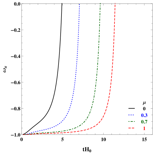
The future evolution of equation of state of field $\omega_{\pi}$ $(=P_{\pi}/\rho_{\pi})$ is shown in fig.4, we notice that more the strength of the slotheon field, more it diverges from the standard coupled quintessence model $(\mu=0)$.

In this section, we constrain the parameters of the model with the assumption of a flat Universe by using the latest observational data.

We consider the Supernovae Type Ia observation which is one of the direct probes for late time acceleration. We have utilized the Union2.1 compilation of the dataset which comprises of 580 datapoints SnIa . It measures the apparent brightness of the Supernovae as observed by us which is related to the luminosity distance $D_{L}$ is the luminosity distance defined as

$\displaystyle D_{L}(z)=(1+z)\int_{0}^{z}\frac{H_{0}dz^{\prime}}{H(z^{\prime})}\,,$

(18)

With this we construct the distance modulus $\mu_{SN}$,which is experimentally measured:

$\displaystyle\mu_{SN}=m-M=5\log D_{L}+25\,,$

(19)

where $m$ and $M$ are the apparent and absolute magnitudes of the Supernovae respectively which are logarithmic measure of flux and luminosity respectively. Other observational probe that has been widely used in recent times to constrain dark energy models is related to the data from the Baryon Acoustic Oscillations measurements bao2 by the large scale galaxy survey. In this case, one needs to calculate the co-moving angular diameter distance $D_{V}$ as follows:

$\displaystyle D_{V}=\left[\frac{z_{BAO}}{H(z_{BAO})}\left(\int_{0}^{z_{BAO}}\frac{dz}{H(z)}\right)^{2}\right]^{\frac{1}{3}}$

(20)

or BAO measurements we calculate the ratio $\frac{D_{V}(z=.35)}{D_{V}(z=.20)}$. This ratio is a relatively model independent quantity and has a measured value $1.736\pm 0.065$.

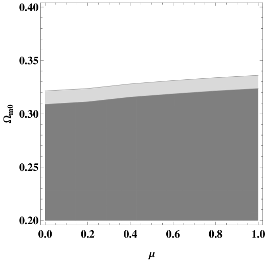
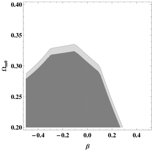
Next we use Hubble data from red-envelope galaxies. 12 measurements of the Hubble parameter H(z) at redshifts $.2<z<1$ are obtained from a high-quality spectra with the Keck-LRIS spectrograph of red-envelope galaxies in 24 galaxy clustersstern . The measurement at $z=0$ was from HST Key project hst .At this point we define the normalised hubble parameter as $h(z)=\frac{H(z)}{H_{0}}$ and utilise it to derive the value of new $h(z)$. Using all these observational data, we constrain the model parameters $\mu$ and $\beta$ to see what is allowed by the observational data. In fig.5 we show the confidence contours in the $(\Omega_{m0},\mu)$ parameter space. We notice that $\mu$ is unconstrained by the data. The confidence contours in parameter space $(\Omega_{m0},\beta)$ is shown in fig.6 for $\mu=0.7$. We notice that $\beta$ is constrained by the data to small values $\beta<0.3$.

In this work we investigated the slotheon gravity in a linear potential. We have shown that cosmological dynamics of this model is similar to the coupled quintessence model at late times, thereby giving an accelerated expansion at recent time. The dynamics of linear potential is such that triggers a collapse of universecollapse . The collapse occur when the field moves down slowly encounters a negative potential energy. The energy density of the universe eventually becomes zero due to which the universe bounces and a collapsing period starts dominating by the kinetic energy of the field. Here we have extended this formalism to the slotheon gravity to study how it is different from the standard quintessence case. When the slotheon gravity strength $\mu=0$, the slotheon field reduces to the standard coupled quintessence. Generally in this case, in an expanding universe, a scalar field will dominate the energy density around the present epoch and drive a period of cosmic acceleration, followed by a period of bounce and collapse. The nature of the collapse is that of the Big Crunch singularity.

We have shown that when the slotheon gravity comes into play $(\mu>0)$, the fate of the universe is similar to that of the standard case. The only difference is the time at which the Big Crunch singularity occurs. It is shown that the collapse is shifted to a distant future in the slotheon gravity and can be made redundant for large value of parameter $\mu$. We have estimated the time of bounce for a particular value of field strength $(\mu=0.7)$ using the slow-roll parameters. Though it gives an approximate result, yet it gives a rough idea about this period and subsequent events following it.

We have also constrained the model parameters $\mu$ and $\beta$ by using the observational data from Supernovae Type Ia, BAO and H(z) measurements. We see that all values of slotheon gravity strength $\mu$ is allowed whereas small values of the coupling constant $\beta$ is preferred by the data.

References

- (1) S. Perlmutter et al., Astrophys. J. 517, 565 (1999); A. G. Riess et al., Astron. J. 116, 1009 (1998).
- (2) D. N. Spergel et al. (WMAP Collaboration), Astrophys. J. Suppl. Ser. 170, 377 (2007).
- (3) S.D. Odintsov, V.K. Oikonomou, Phys. Rev. D 94 064022 (2016); S. Nojiri, S.D. Odintsov, V.K. Oikonomou, Phys. Rev. D 93 084050 (2016); S.D. Odintsov, V.K. Oikonomou, Phys. Rev. D 92 024016 (2015); S.D. Odintsov, V.K. Oikonomou, Phys. Rev. D 90 124083 (2014).
- (4) V. Sahni and A. A. Starobinsky, Int. J. Mod. Phys. D9, 373 (2000); S. M. Carroll, Living Rev. Relativity 4, 1 (2001); T. Padmanabhan, Phys. Rep. 380, 235 (2003); P. J. E. Peebles and B. Ratra, Rev. Mod. Phys. 75, 559 (2003); E. V. Linder, J. Phys. Conf. Ser. 39, 56 (2006); L. Perivolaropoulos, AIP Conf. Proc. 848, 698 (2006).
- (5) E. J. Copeland, M. Sami, and S. Tsujikawa, Int. J. Mod. Phys. D 15, 1753 (2006).
- (6) E. V. Linder, Gen. Relativ. Gravit. 40, 329 (2008); J. Frieman, M. Turner, and D. Huterer, Annu. Rev. Astron. Astrophys. 46, 385 (2008).
- (7) R. R. Caldwell, R. Dave, and P. J. Steinhardt, Phys. Rev. Lett. 80,1582 (1998); T. Chiba, T. Okabe, and M. Yamaguchi, Phys. Rev. D 62, 023511 (2000).
- (8) I. Zlatev, L. M. Wang, and P. J. Steinhardt, Phys. Rev. Lett. 82, 896 (1999); P. J. Steinhardt, L. M. Wang, and I. Zlatev, Phys. Rev. D 59, 123504 (1999); L. Amendola, Phys. Rev. D 62, 043511 (2000).
- (9) C. Armendariz-Picon, V. Mukhanov, and P. J. Steinhardt, Phys. Rev. Lett. 85, 4438 (2000); Phys. Rev. D 63, 103510 (2001); T. Chiba, T. Okabe, and M. Yamaguchi, Phys. Rev. D 62, 023511 (2000).
- (10) R. Kallosh, J. Kratochvil, A. Linde, E. Linder, and M. Shmakova, J. Cosmol. Astropart. Phys. 10, 015 (2003); Y. Wang et al, Cosmol. Astropart. Phys.12, 006 (2004); P. P. Avelino, C. J. A. P. Martins, and J. C. R. E. Oliveira, Phys. Rev. D 70, 083506 (2004); P. P. Avelino, Phys. Lett. B. 611, 15 (2005).
- (11) S. Capozziello, Int. J. Mod. Phys. D 11 483 (2002); S. Capozziello, S. Carloni and A. Troisi, Recent Res. Dev. Astron. Astrophys. 1 625 (2003); Shin’ichi Nojiri, Sergei D. Odintsov, Phys. Rept. 505 59-144 (2011).
- (12) A. Nicolis, R. Rattazzi, and E. Trincherini, Phys. Rev. D 79, 064036 (2009); C. Deffayet, G. Esposito-Farese, and A. Vikman, Phys. Rev. D 79, 084003 (2009).
- (13) G. R. Dvali, G. Gabadadze and M. Porrati, Phys. Lett. B 485, 208 (2000).
- (14) G. W. Hordenski, Int. J. Theor. Phys. 10, 363-384 (1974).
- (15) R. Gannouji and M. Sami, Phys. Rev. D 82, 024011 (2010); A. Ali, R. Gannouji, and M. Sami, Phys. Rev. D 82, 103015 (2010).
- (16) A. Ali, R. Gannouji, M. W. Hossain, and M. Sami, Phys. Lett. B 718, 5 (2012).
- (17) M. Shahalam, S. K. J. Pacif, R. Myrzakulov, Eur. Phys. J. C 76, 410 (2016).
- (18) C. Germani, L. Martucci, and P. Moyassari, Phys. Rev. D 85, 103501 (2012).
- (19) C. Germani, Phys. Rev. D 86, 104032 (2012).
- (20) D. Adak and K. Dutta, Phys. Rev. D90, 043502 (2014).
- (21) D. Adak, A. Ali and D. Majumdar, Phys. Rev. D88, 024007 (2013).
- (22) Sudhakar Panda, Yoske Sumitomo, Sandip P. Trivedi, Phys. Rev. D83, 083506 (2011).
- (23) Robert J. Scherrer and A. A. Sen, Phys. Rev. D 77, 083515 (2008); L. Perivolaropoulos Phys. Rev. D 71, 063503 (2005).
- (24) Ricardo Z. Ferreira and Pedro P. Avelino, arXiv:1508.00631 [astro-ph.CO].
- (25) N. Suzuki et al, Astrophys. J. 746 (2012) 85.
- (26) W. J. Percival et al, Mon. Not. Roy. Astron. Soc. 401, 2148 (2010).
- (27) D. Stern, R. Jimenez, L. Verde, M. Kamionkowski and S. Adam, JCAP 1002,(2010) 008.
- (28) W. L. Freedman et al. [HST Collaboration], Astrophys. J. 553 (2001) 47.