Boundary conditions effects by Discontinuous Galerkin Solvers for Boltzmann-Poisson models of Electron Transport

José A. Morales Escalante Institute for Computational
Engineering and Sciences (ICES)
The University of Texas at Austin
Austin, Texas 78712-1229
Email: jmorales@ices.utexas.edu Irene M. Gamba Department of Mathematics and ICES
The University of Texas at Austin
Austin, Texas 78712-1229
Email: gamba@math.utexas.edu

Abstract

In this paper we perform, by means of Discontinuous Galerkin (DG) Finite Element Method (FEM) based numerical solvers for Boltzmann-Poisson (BP) semiclassical models of hot electronic transport in semiconductors, a numerical study of reflective boundary conditions in the BP system, such as specular reflection, diffusive reflection, and a mixed convex combination of these reflections, and their effect on the behavior of the solution. A boundary layer effect is observed in our numerical simulations for the kinetic moments related to diffusive and mixed reflection.

I Introduction

June 30, 2014

The dynamics of electron transport in modern semiconductor devices can be described by the semiclassical Boltzmann-Poisson (BP) model:

\frac{\partial f_{i}}{\partial t}+\frac{1}{\hbar}\nabla_{\vec{k}}\,\varepsilon_{i}(\vec{k})\cdot\nabla_{\vec{x}}f_{i}-\frac{q_{i}}{\hbar}\vec{E}\cdot\nabla_{\vec{k}}f_{i}=\sum_{j}Q_{i,j}

(I.1)

\nabla_{\vec{x}}\cdot\left(\epsilon\,\nabla_{\vec{x}}V\right)=\sum_{i}q_{i}\rho_{i}-N(\vec{x}),\vec{E}=-\nabla_{\vec{x}}V

(I.2)

$f_{i}(\vec{x},\vec{k},t)$ is the probability density function (pdf) over phase space $(\vec{x},\vec{k})$ of a carrier in the $i$ -th energy band in position $\vec{x}$ , with crystal momentum $\hbar\vec{k}$ at time $t$ . The collision operators $Q_{i,j}(f_{i},f_{j})$ model $i$ -th and $j$ -th carrier recombinations, collisions with phonons or generation effects. $\vec{E}(\vec{x},t)$ is the electric field, $\varepsilon_{i}(\vec{k})$ is the $i$ -th energy band surface, the $i$ -th charge density $\rho_{i}(t,\vec{x})$ is the k-average of $f_{i}$ , and $N(\vec{x})$ is the doping profile.

Deterministic solvers for the BP system using Discontinuous Galerkin (DG) FEM have been proposed in [1, 2] to model electron transport along the conduction band for 1D diodes and 2D double gate MOSFET devices. In [1], the energy band $\varepsilon(\vec{k})$ model used was the nonparabolic Kane band model. These solvers are shown to be competitive with Direct Simulation Monte Carlo (DSMC) methods [1]. The energy band models used in [2] were the Kane and Brunetti, $\varepsilon(|\vec{k}|)$ analytical models, but implemented numerically for benchmark tests.

Boundary conditions (BC) for BP models in $(\vec{x},\vec{k})$ -boundaries vary according to the considered device and physical situation. For example, considering electron transport along a single conduction band:

Charge neutrality boundary conditions in 1D and 2D devices are given by:

f_{out}(t,\vec{x},\vec{k})|_{\Gamma}=N_{D}(\vec{x})\frac{f_{in}(t,\vec{x},\vec{k})|_{\Gamma}}{\rho_{in}(t,\vec{x})},\quad\vec{x}\in\Gamma\subseteq\partial\Omega_{\vec{x}}

(I.3)

Specular reflection BC over the Neumann Inflow Boundary
$\Gamma_{N}^{-}=\{(\vec{x},\vec{k}):\vec{x}\in\Gamma_{N},\,\vec{k}\in\Omega_{k},\,\nabla_{\vec{k}}\,\varepsilon(\vec{k})\cdot\eta(\vec{x})<0\}$ , with outward unit normal $\eta(\vec{x})$ (the Neumann boundary $\Gamma_{N}$ usually defines insulating boundaries) is imposed by:

f^{spec}(\vec{x},\vec{k},t)=f(\vec{x},\vec{k}^{\prime},t)\quad\mbox{for}\quad(\vec{x},\vec{k})\in\Gamma_{N}^{-},\quad t>0.

(I.4)

for $\vec{k^{\prime}}\quad\mbox{s.t.}\quad\nabla_{\vec{k}}\varepsilon(\vec{k}^{\prime})=\nabla_{\vec{k}}\varepsilon(\vec{k})-2(\nabla_{\vec{k}}\varepsilon(\vec{k})\cdot\eta(\vec{x}))\eta(\vec{x}).$

Diffusive reflection BC is known in the kinetic theory of gas dynamics. The distribution function at the Inflow boundary is proportional to a Maxwellian [4]. For $(\vec{x},\vec{k})\in\Gamma_{N}^{-}$ :

f^{diff}(\vec{x},\vec{k},t)=Ce^{-\varepsilon(\vec{k})/K_{B}T}\int_{\nabla_{\vec{k}}\varepsilon(\vec{k})\cdot\eta>0}\nabla_{\vec{k}}\varepsilon(\vec{k})\cdot\eta(\vec{x})fd\vec{k}

(I.5)

Mixed reflection BC models the reflection of the electrons from a rough boundary, giving by the reflected wave for convex combination of specular and diffuse components

$f(\vec{x},\vec{k})=p\,f^{spec}(\vec{x},\vec{k})+(1-p)f^{diff}(\vec{x},\vec{k}),\quad(\vec{x},\vec{k})\in\Gamma_{N}^{-}$

where the probability $p$ is sometimes called the specularity parameter. It can either be constant, or be a function of the momentum $p(\vec{k})$ , as in [5].

I-A BP system with $\vec{k}$ coordinate transformation assuming a Kane Energy Band

The Kane Energy Band Model is a dispersion relation between the conduction energy band $\varepsilon$ (measured from a local minimum) and the norm of the electron wave vector $|k|$ , given by the analytical function ( $\alpha$ is a constant parameter, $m^{*}$ is the electron reduced mass for Si, and $\hbar$ is Planck’s constant):

\varepsilon(1+\alpha\varepsilon)=\frac{\hbar^{2}|k|^{2}}{2m^{*}}

(I.6)

For our preliminary numerical studies we will use a Boltzmann-Poisson model as in [1], in which the conduction energy band is assumed to be given by a Kane model.

We use the following dimensionalized variables, with the related characteristic parameters:

$\displaystyle t={\mathrm{t}}/{t_{*}},(x,y)={\vec{x}}/{\ell_{*}},\ell_{*}=10^{-6}m$ , $t_{*}=10^{-12}s$ , $V_{*}=1\mbox{V}$

A transformed Boltzmann transport equation is used as in [1] as well, where the coordinates used to describe $\vec{k}$ are: $\mu$ , the cosine of the polar angle, the azimuthal angle $\varphi$ , and the dimensionless Kane Energy $w={\varepsilon}/{K_{B}T}$ ( $K_{B}$ is Boltzmann’s constant, $T$ is the lattice temperature, and $\alpha_{K}=\alpha{K_{B}T}$ ):

\vec{k}=\vec{k}(w,\mu,\varphi)=

(I.7)

$\frac{\sqrt{2m^{*}k_{B}T_{L}}}{\hbar}\sqrt{w(1+\alpha_{K}w)}\left(\mu,\sqrt{1-\mu^{2}}\cos\varphi,\sqrt{1-\mu^{2}}\sin\varphi\right)$

A new unknown function $\Phi$ is used in the transformed Boltzmann Eq. [1], which is proportional to the Jacobian of the transformation and to the density of states:

\Phi(t,x,y,w,\mu,\varphi)=s(w)f(\mathrm{t},\vec{x},\vec{k})\,,

(I.8)

where $s(w)=\sqrt{w(1+\alpha_{K}w)}(1+2\alpha_{K}w).$

The transformed Boltzmann transport equation for $\Phi$ in [1] is:

{\partial_{t}\Phi}+{\nabla_{\left(x,y,w,\mu,\varphi\right)}}\cdot\left(\Phi\vec{g}\right)=C(\Phi)

(I.9)

Regarding $\vec{g}=(g_{1},g_{2},g_{3},g_{4},g_{5})$ , the functions $g_{i}$ , for $i=1,2$ are proportional to the $k_{x},\,k_{y}$ cartesian components of the electron group velocity $\frac{\partial w}{\partial\vec{k}}$ written as functions of the coordinates $w$ , $\mu$ , $\varphi$ . The functions $g_{i}$ , for $i=3,4,5$ , represent the transport in $\vec{k}$ -space due to the electric field, time and position dependent.

The right hand side of (I.9) is the collision operator, after having applied the Fermi Golden Rule for electron-phonon scattering, that depends on the energy differences between transition states,

	$\displaystyle C(\Phi)(t,x,y,w,\mu,\varphi)=$
	$\displaystyle\ s(w)\left\{c_{0}\int_{0}^{\pi}\!\!d\varphi^{\prime}\int_{-1}^{1}\!d\mu^{\prime}\>\Phi(t,x,y,w,\mu^{\prime},\varphi^{\prime})\right.$
	$\displaystyle\left.\ \ +\int_{0}^{\pi}\!\!d\varphi^{\prime}\int_{-1}^{1}\!d\mu^{\prime}\>[c_{+}\Phi(t,x,y,w+\gamma,\mu^{\prime},\varphi^{\prime})\right.$
	$\displaystyle\left.\ \ \qquad\qquad\qquad+c_{-}\Phi(t,x,y,w-\gamma,\mu^{\prime},\varphi^{\prime})]\right\}$
	$\displaystyle-2\pi[c_{{}_{0}}s(w)+c_{{}_{+}}s(w-\gamma)+c_{{}_{-}}s(w+\gamma)]\Phi(t,x,y,w,\mu,\varphi),$

with the dimensionless parameters $\gamma=\frac{\hbar\omega_{p}}{k_{B}T_{L}},$

\displaystyle(c_{0},c_{+},c_{-})=\frac{2m^{*}\,t_{*}}{\hbar^{3}}\sqrt{2\,m^{*}\,k_{B}T_{L}}\left(K_{0},(n_{q}+1)K,n_{q}K\right),

(I.10)

The electron density is:

\displaystyle n(t_{*}t,\ell_{*}x,\ell_{*}y)=\int_{\scriptstyle\mbox{\iams\char 82\relax}^{3}}f\>d\mathbf{k}=\left(\frac{\sqrt{2\,m^{*}k_{B}T_{L}}}{\hbar}\right)^{\!\!3}\rho(t,x,y)\,,

where

\rho(t,x,y)=\int_{0}^{+\infty}\!\!dw\int_{-1}^{1}\!d\mu\int_{0}^{\pi}\!\!d\varphi\>\Phi(t,x,y,w,\mu,\varphi)\,.

(I.11)

Hence, the dimensionless Poisson equation is

\frac{\partial}{\partial x}\left(\epsilon_{r}\frac{\partial\Psi}{\partial x}\right)+\frac{\partial}{\partial y}\left(\epsilon_{r}\frac{\partial\Psi}{\partial y}\right)=c_{p}\left[\rho(t,x,y)-\mathcal{N}_{D}(x,y)\right]

(I.12)

$\mathcal{N}_{D}(x,y)=\left(\frac{\sqrt{2\,m^{*}k_{B}T_{L}}}{\hbar}\right)^{\!\!-3}N_{D}(\ell_{*}x,\ell_{*}y),\,$
$c_{p}=\left(\frac{\sqrt{2\,m^{*}k_{B}T_{L}}}{\hbar}\right)^{\!\!3}\frac{\ell_{*}^{2}q}{\epsilon_{0}}.$

II Numerics: Discontinuous Galerkin Method for BP and Boundary Conditions Implementation

II-A DG Method Formulation

The DG Method formulation for the transformed Boltzmann Eq. that we consider in this work was developed in [1], to which we refer for more details. We summarize the basics of the formulation below.

II-A1 Domain - 2d- $\vec{x}$ Device, 3d- $\vec{k}$ Space

The domain of the devices to be considered can be represented by means of a rectangular grid in both position and momentum space, i.e.:

$i=1:N_{x},j=1:N_{y},k=1:N_{w},m=1:N_{\mu},n=1:N_{\varphi}$ ,

$\Omega_{I}=\left[x_{i-\frac{1}{2}},x_{i+\frac{1}{2}}\right]\times\left[y_{j-\frac{1}{2}},y_{j+\frac{1}{2}}\right]\times\left[w_{k-\frac{1}{2}},w_{k+\frac{1}{2}}\right]\times\left[\mu_{m-\frac{1}{2}},\mu_{m+\frac{1}{2}}\right]\times\left[\varphi_{n-\frac{1}{2}},\varphi_{n+\frac{1}{2}}\right]$

$x_{i\pm\frac{1}{2}}=x_{i}\pm\frac{\Delta x_{i}}{2}\,,\quad y_{j\pm\frac{1}{2}}=y_{j}\pm\frac{\Delta y_{j}}{2}\,,\quad w_{k\pm\frac{1}{2}}=w_{k}\pm\frac{\Delta w_{k}}{2}\,$

$\mu_{m\pm\frac{1}{2}}=\mu_{m}\pm\frac{\Delta\mu_{m}}{2}\,,\quad\varphi_{n\pm\frac{1}{2}}=\varphi_{n}\pm\frac{\Delta\varphi_{n}}{2}.$

$\Phi_{h}$ will denote the Piecewise Linear Approximation of $\Phi$ in a given cell $\mathring{\Omega}_{I}$ , with the multi-index $I=ijkmn$ :

$\Phi_{h}\,=\,T_{ijkmn}(t)+X_{ijkmn}(t)\,\frac{(x-x_{i})}{\Delta x_{i}/2}+Y_{ijkmn}(t)\,\frac{(y-y_{j})}{\Delta y_{j}/2}+\\ W_{ijkmn}(t)\,\frac{(w-w_{k})}{\Delta w_{k}/2}+M_{ijkmn}(t)\,\frac{(\mu-\mu_{m})}{\Delta\mu_{m}/2}+P_{ijkmn}(t)\,\frac{(\varphi-\varphi_{n})}{\Delta\varphi_{n}/2}$

II-A2 Discontinous Galerkin (DG) Formulation for the Transformed Boltzmann - Poisson (BP) System

On a cartesian grid, for each element $\Omega_{I}$ , find $\Phi_{h}$ in $V_{h}$ (piecewise linear polynomial space) s.t. for any test function $v_{h}\in V_{h}$

	$\displaystyle\displaystyle\int_{\Omega_{I}}\frac{\partial\Phi_{h}}{\partial t}v_{h}d\Omega-\int_{\Omega_{I}}\frac{\partial{v_{h}}}{\partial x}\left(g_{1}\,\Phi_{h}\right)d\Omega$
	$\displaystyle\hskip-30.0pt\mbox{ }-\int_{\Omega_{I}}\frac{\partial{v_{h}}}{\partial y}\left(g_{2}\,\Phi_{h}\right)d\Omega-\int_{\Omega_{I}}\frac{\partial v_{h}}{\partial w}\left(g_{3}\,\Phi_{h}\right)d\Omega$
	$\displaystyle\hskip-30.0pt\mbox{ }-\int_{\Omega_{I}}\frac{\partial v_{h}}{\partial\mu}\left(g_{4}\,\Phi_{h}\right)d\Omega-\int_{\Omega_{I}}\frac{\partial v_{h}}{\partial\varphi}\left(g_{5}\,\Phi_{h}\right)d\Omega$
	$\displaystyle\hskip-30.0pt\mbox{ }+F_{x}^{+}-F_{x}^{-}+F_{y}^{+}-F_{y}^{-}+F_{w}^{+}-F_{w}^{-}+F_{\mu}^{+}-F_{\mu}^{-}$
	$\displaystyle\mbox{ }+F_{\varphi}^{+}-F_{\varphi}^{-}=\int_{\Omega_{I}}C(\Phi_{h})v_{h}d\Omega,$

$F^{\pm}$ ’s denote boundary integrals, for which the value of $\Phi$ at the boundary is given by the Numerical Upwind Flux rule.

II-A3 Algorithm for DG-BP, from $t^{n}$ to $t^{n+1}$

(Dynamic Extension of Gummel Iteration Map)

1.- Compute electron density $\rho$ , use it to…
2.- Solve Poisson Eq. (by Local DG) for the potential, then get the electric field $\vec{E}$ . Compute then $g_{i}$ ’s transport terms.
3.- Solve by DG the transport part of Boltzmann Equation. Method of lines (ODE system) for the time-dependent coefficients of $\Phi_{h}$ (degrees of freedom) obtained.
4.-Evolve ODE system by time stepping from $t^{n}$ to $t^{n+1}$ .
(If partial time step necessary, repeat Step 1 to 3 as needed).

II-B Numerical Implementation of Reflection Boundary Conditions (BC) by DG schemes

II-B1 Specular Reflection BC

Specular reflection at boundaries $y=0,\,L_{y}$ is expressed in angular coordinates by:

$\Phi^{spec}_{h}(t,x,y,w,\mu,\varphi)=\Phi_{h}(t,x,-y,w,\mu,\pi-\varphi)\,$

Defining $n^{\prime}=N_{\varphi}-n+1$ , $\,I=i0kmn,\,I^{\prime}=i1kmn^{\prime}$ ,
if $(x,y,w,\mu,\varphi)\in\Omega_{I}$ , then $(x,-y,w,\mu,\pi-\varphi)\in\Omega_{I^{\prime}}$ . This implies that the $\Phi_{h}$ coefficients satisfy, taking $\Delta\varphi_{n^{\prime}}=\Delta\varphi_{n}$ :

$T_{I}=T_{I^{\prime}},\quad X_{I}=X_{I^{\prime}},\quad Y_{I}=-Y_{I^{\prime}},\\ W_{I}=W_{I^{\prime}},\quad M_{I}=M_{I^{\prime}},\quad P_{I}=-P_{I^{\prime}}.$

II-B2 Diffusive Reflection BC

We define the DG approximate diffusive function $\Phi_{h}^{diff}\in V_{h}^{1}$ as follows:

Use the projection $\Phi_{h}:=\Pi\Phi(t,x,y,w,\mu,\varphi)\in V_{h}^{1}$ and set

$\sigma_{h}(x,y,t):=\int_{\pm\cos\varphi\geq 0}|g_{2}|\,\Phi_{h}\,dwd\mu d\varphi\,\in V_{h}^{1}.$ Next, since $\Phi^{diff}=C\,\sigma_{h}\,e^{-w}s(w)$ , then set the approximate by projecting $\Phi_{h}^{diff}:=\Pi\Phi^{diff}\in V_{h}^{1}.$

II-B3 Mixed Reflection BC

These conditions are numerically approximated by taking the convex combination:
$\Phi^{mr}_{h}=p(\vec{k})\,\Phi_{h}^{spec}+\big{(}1-p(\vec{k})\big{)}\Phi_{h}^{diff}\,$ of specular and diffusive reflections respectively, where the we use the momentum-dependent specularity parameter [5] given by the probability $p(\vec{k})=e^{-4L_{r}^{2}|k|^{2}\cos^{2}\Theta}=\exp(-4l_{r}^{2}w(1+\alpha_{K}w)\sin^{2}\varphi)=p(w,\varphi),$ with $l_{r}$ the (normalized) rms rough interface height [7].

III Preliminary Numerical Results

In our preliminary numerical simulations we consider a 2D n bulk Silicon with rectangular geometry in $(x,y)$ (width: $L_{x}=0.15\mu m$ , height: $L_{y}=12nm$ ) to completely isolate the effect of the reflective boundary conditions on the kinetic moments for this benchmark case. The respective domain in $\vec{k}(w,\mu,\varphi)$ is rectangular in 3D.

Initial Condition: $\left.\Phi(w)\right|_{t=0}\propto Ne^{-w}s(w)$ . Final Time: 1.0ps
Boundary Conditions in $\vec{k}$ -space: a cut-off is set at $w=w_{max}$ with $\Phi$ machine zero.
This is the only BC needed in $\vec{k}(w,\mu,\varphi)$ , since the transport normal to the boundary is analitically zero at boundaries related to the following ’singular points’:
At $w=0$ , $g_{3}=0$ . At $\mu=\pm 1$ , $g_{4}$ = 0. At $\varphi=0,\pi$ , $g_{5}$ = 0.
BC in $\vec{x}$ -space: we set neutral charges at boundaries
$x=0,\,x=0.15\mu m$ .
The Potential-bias BC is set as either:
$\Delta V=\left.V\right|_{x=0.15\mu m}-\left.V\right|_{x=0}=0.5,1.0,\,$ or $\,1.5$ Volts.
The reflection BC, either specular, diffusive or mixed, are set at $y=0,y=12nm$ .
The number of cells used in the simulation were:
$N_{x}=24,\,N_{y}=12,\,N_{w}=30,\,N_{\mu}=8,N_{\varphi}=6$ .

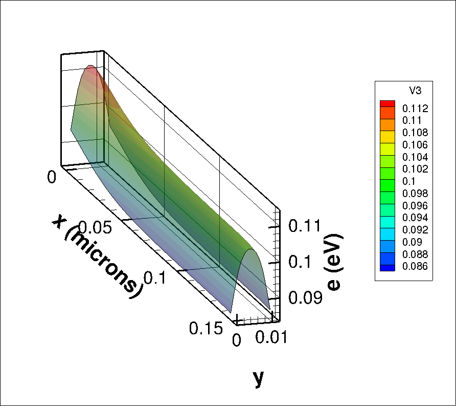
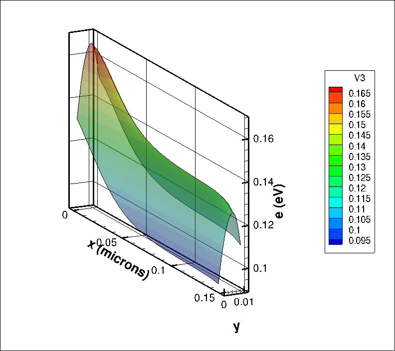
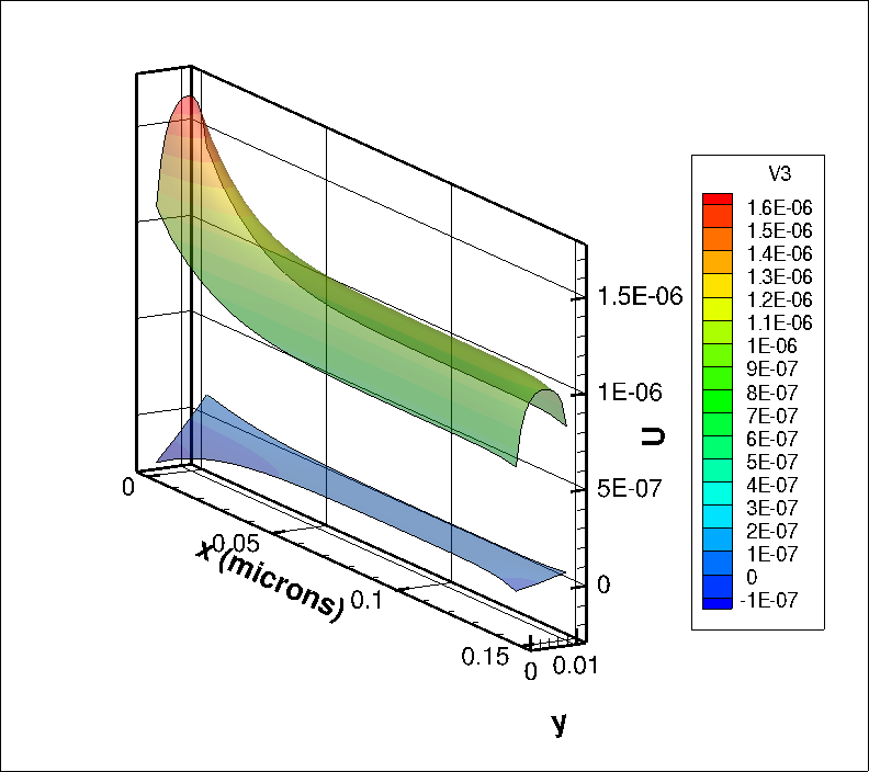
We present plots of the Average Energy $e$ and Momentum $U$ vs. Position $(x,y)$ at the final time of $t=1.0$ ps with a $\Delta V=1.0$ Volt bias for the different specular, diffusive and mixed reflection BC implemented. A boundary layer was observed in the plots of the average density, average energy, and average momentum for the diffusive and mixed reflection cases in the boundaries where these reflection conditions are applied, compared to the specular case in which these moments are constant w.r.t. position for the benchmark case considered. Boundary layers were also observed for the biases of $\Delta V=0.5,1.5$ Volts, obtaining higher values for average energy and momentum when increasing the bias as expected. A point to mention is that a DSMC solver for BP would have a hard time to resolve the details of the momentum to the scales present in the momentum plots for our deterministic solver.

Refer to caption — Figure III.1: Mean energy $e$ (eV) vs. Position $(x,y)$ in $(\mu m)$ plots for Specular (top) and Diffusive (right above) Reflection.

IV Conclusion

A Boundary Layer effect was observed in the Kinetic Moments related to the Diffusive and Mixed Reflection cases. Work in Progress is related to the case of a 2D double gate MOSFET device. An extended version with more details and results will be presented [6]. Future work will consider a study of reflective BC on DG solvers where an EPM full band is numerically implemented for 2D devices in $\vec{x}$ .

Acknowledgment

The authors have been partially funded by NSF grants CHE-0934450, DMS-1109625, and DMS-RNMS-1107465. The first author was funded by a NIMS fellowship given by ICES, U.Texas-Austin.

References

[1] Y. Cheng, I. M. Gamba, A. Majorana, and C.W. Shu A Discontinous Galerkin solver for Boltzmann-Poisson systems in nano-devices, CMAME 198, 3130-3150 (2009).
[2] Y. Cheng, I. M. Gamba, A. Majorana and C.-W. Shu, A discontinuous Galerkin solver for full-band Boltzmann-Poisson models, IWCE13 Proceedings (2009).
[3] Y. Sone, Molecular Gas Dynamics: Theory, Techniques, and Applications, Birkhauser (2007).
[4] A. Jungel, Transport Equations for Semiconductors, Springer Verlag (2009).
[5] S. Soffer Statistical Model for the size effect in Electrical Conduction, Journal of Applied Physics 38 1710 (1967).
[6] J. Morales Escalante, I. M. Gamba, Discontinuous Galerkin schemes for diffusive reflection for Boltzmann-Poisson electron transport with rough boundaries, in preparation (2014).
[7] Degarmo, E. P.; Black, J.; Kohser, R.A.; Materials and Processes in Manufacturing (9th ed.), Wiley, p. 223, (2003).