Breaking the Cubic Barrier for All-Pairs Max-Flow:
Gomory-Hu Tree in Nearly Quadratic Time
Abstract
In 1961, Gomory and Hu showed that the All-Pairs Max-Flow problem of computing the max-flow between all pairs of vertices in an undirected graph can be solved using only calls to any (single-pair) max-flow algorithm. Even assuming a linear-time max-flow algorithm, this yields a running time of , which is when . While subsequent work has improved this bound for various special graph classes, no subcubic-time algorithm has been obtained in the last 60 years for general graphs. We break this longstanding barrier by giving an -time algorithm on general, weighted graphs. Combined with a popular complexity assumption, we establish a counter-intuitive separation: all-pairs max-flows are strictly easier to compute than all-pairs shortest-paths.
Our algorithm produces a cut-equivalent tree, known as the Gomory-Hu tree, from which the max-flow value for any pair can be retrieved in near-constant time. For unweighted graphs, we refine our techniques further to produce a Gomory-Hu tree in the time of a poly-logarithmic number of calls to any max-flow algorithm. This shows an equivalence between the all-pairs and single-pair max-flow problems, and is optimal up to poly-logarithmic factors. Using the recently announced -time max-flow algorithm (Chen et al., March 2022), our Gomory-Hu tree algorithm for unweighted graphs also runs in -time.
Historical note:
The first version of this paper (arXiv:2111.04958) titled “Gomory-Hu Tree in Subcubic Time” (Nov. 9, 2021) broke the cubic barrier but only claimed a time bound of . The second version (Nov. 30, 2021) optimized one of the ingredients (Section 2) and gave the time bound. The latter optimization was discovered independently by Zhang [Zha21].
1 Introduction
The edge connectivity of a pair of vertices in an undirected graph is defined as the minimum weight of edges whose removal disconnects and in the graph. Such a set of edges is called an mincut, and by duality, its value is equal to that of an max-flow. Consequently, the edge connectivity of a vertex pair is obtained by running a max-flow algorithm, and by extension, the edge connectivity for all vertex pairs can be obtained by calls to a max-flow algorithm. (Throughout, and denote the number of vertices and edges in the input graph , where maps edges to non-negative integer weights. We denote the maximum edge weight by .)
Definition 1.1 (The All-Pairs Max-Flow (APMF) Problem).
Given an undirected edge-weighted graph, return the edge connectivity of all pairs of vertices.
Remarkably, Gomory and Hu [GH61] showed in a seminal work in 1961 that one can do a lot better than this naïve algorithm. In particular, they introduced the notion of a cut tree (later called Gomory-Hu tree, which we abbreviate as GHtree) to show that max-flow calls suffice for finding the edge connectivity of all vertex pairs.
Theorem 1.2 (Gomory-Hu (1961)).
For any undirected edge-weighted graph , there is a cut tree (or GHtree), which is defined as a tree on the same set of vertices such that for all pairs of vertices , the mincut in is also an mincut in and has the same cut value. Moreover, such a tree can be computed using max-flow calls.111These max-flow calls are on graphs that are contractions of , and thus no larger than .
Since their work, substantial effort has gone into obtaining better GHtree algorithms, and faster algorithms are now known for many restricted graph classes, including unweighted graphs [BHKP07, KL15, AKT21b], simple graphs [AKT21c, AKT21a, LPS21, Zha22, AKT22], planar graphs [BSW15], surface-embedded graphs [BENW16], bounded treewidth graphs [ACZ98, AKT20], and so on (see Table 1 and the survey [Pan16]). Indeed, GHtree algorithms are part of standard textbooks in combinatorial optimization (e.g., [AMO93, CCPS97, Sch03]) and have numerous applications in diverse areas such as networks [Hu74], image processing [WL93], and optimization [PR82]. They have also inspired entire research directions as the first example of a sparse representation of graph cuts, the first non-trivial global min-cut algorithm, the first use of submodular minimization in graphs, and so forth.
In spite of this attention, Gomory and Hu’s 60-year-old algorithm has remained the state of the art for constructing a GHtree in general, weighted graphs (or equivalently for APMF, due to known reductions [AKT20, LPS21] showing that any APMF algorithm must essentially construct a GHtree). Even if we assume an optimal -time max-flow algorithm, the Gomory-Hu algorithm takes time, which is when . Breaking this cubic barrier for the GHtree problem has been one of the outstanding open questions in the graph algorithms literature.
In this paper, we break this longstanding barrier by giving a GHtree algorithm that runs in -time for general, weighted graphs.
Theorem 1.3.
There is a randomized Monte Carlo algorithm for the GHtree (and APMF) problems that runs in time in general, weighted graphs.
Remarks:
1. As noted earlier (and similar to state-of-the-art max-flow algorithms), we assume throughout the paper that edge weights are integers in the range . Throughout, the notation hides poly-logarithmic factors in and .
2. Our result is unconditional, i.e., it does not need to assume a (near/almost) linear-time max-flow algorithm. We note that concurrent to our work, an almost-linear time max-flow algorithm has been announced [CKL+22]. Our improvement of the running time of GHtree/APMF is independent of this result: even with this result,
the best GHtree/APMF bound was which is between and depending on the value of , and we improve it to . Moreover, we stress that we do not need any recent advancement in max-flow algorithms for breaking the cubic barrier: even using the classic Goldberg-Rao max-flow algorithm [GR98]
in our (combinatorial) algorithm solves GHtree/APMF in subcubic time.
Our techniques also improve the bounds known for the GHtree problem in unweighted graphs, and even for simple graphs. For unweighted graphs, the best previous results were obtained by Bhalgat et al. [BHKP07] and by Karger and Levine [KL15], and an incomparable result that reduces the GHtree problem to max-flow calls [AKT21b]. There has recently been much interest and progress on GHtree in simple graphs as well [AKT21c, AKT21a, LPS21, Zha22, AKT22], with the current best running time being .
We give a reduction of the GHtree problem in unweighted graphs to calls of any max-flow algorithm. Note that this reduction is nearly optimal (i.e., up to the poly-log factor) since the all-pairs max-flow problem is at least as hard as finding a single-pair max-flow. Using the recent -time max-flow algorithm [CKL+22], this yields a running time of for the GHtree problem in unweighted graphs.
Theorem 1.4.
There is a randomized Monte Carlo algorithm for the GHtree problem that runs in time in unweighted graphs.
APMF vs APSP.
Our results deliver a surprising message to a primordial question in graph algorithms: What is easier to compute, shortest paths or max-flows? Ignoring factors, the single-pair versions are both solvable in linear-time and therefore equally easy; albeit, the shortest path algorithm [Dij59] is classical, elementary, and fits on a single page, whereas the max-flow algorithm [CKL+22] is very recent, highly non-elementary, and requires more than a hundred pages to describe and analyze. This and nearly all other evidence had supported the consensus that max-flows are at least as hard as (if not strictly harder than) shortest paths, and perhaps this can be established by looking at the more general all-pairs versions: APMF and APSP (All-Pairs Shortest-Paths). Much effort had gone into proving this belief (APMF APSP) using the tools of fine-grained complexity [AVY15, KT18, AGI+19, AKT21b, AKT20], with limited success: it was shown that (under popular assumptions) APMF is strictly harder than APSP in directed graphs, but the more natural undirected setting remained open. The first doubts against the consensus were raised in the aforementioned algorithms for APMF in simple (unweighted) graphs that go below the bound of APSP [Sei95] (where [AW21] denotes the fast matrix multiplication exponent). But if, as many experts believe, then the only conclusion is that APMF and APSP are equally easy in simple graphs. In general (weighted) graphs, however, one of the central conjectures of fine-grained complexity states that the cubic bound for APSP cannot be broken (even if ). Under this “APSP Conjecture”, Theorem 1.3 proves that APMF is strictly easier than APSP! Alternatively, if one still believes that APMF APSP, then our paper provides strong evidence against the APSP Conjecture and against the validity of the dozens of lower bounds that are based upon it (e.g., [RZ04, WW18, AW14, AGW15, Sah15, AD16, BGMW20]) or upon stronger forms of it (e.g., [BT17, BDT16, CMWW19, ACK20, GMW21]).
1.1 Related Work
Algorithms.
Before this work, the time complexity of constructing a Gomory-Hu tree in general graphs has improved over the years only due to improvements in max-flow algorithms. An alternative algorithm for the problem was discovered by Gusfield [Gus90], where the max-flow queries are made on the original graph (instead of on contracted graphs). This algorithm has the same worst-case time complexity as Gomory-Hu’s, but may perform better in practice [GT01]. Many faster algorithms are known for special graph classes or when allowing a -approximation, see Table 1 for a summary. Moreover, a few heuristic ideas for getting a subcubic complexity in social networks and web graphs have been investigated [AIS+16].
| Restriction | Running time | Reference |
|---|---|---|
| General | Gomory and Hu [GH61] | |
| Bounded Treewidth* | Arikati, Chaudhuri, and Zaroliagis [ACZ98] | |
| Unweighted | Karger and Levine [KL15] | |
| Unweighted | Bhalgat, Hariharan, Kavitha, and Panigrahi [BHKP07] | |
| Planar | Borradaile, Sankowski, and Wulff-Nilsen [BSW15] | |
| Bounded Genus | Borradaile, Eppstein, Nayyeri, and Wulff-Nilsen [BENW16] | |
| Unweighted | Abboud, Krauthgamer, and Trabelsi [AKT21b] | |
| -Approx* | Abboud, Krauthgamer, and Trabelsi [AKT20] | |
| Bounded Treewidth | Abboud, Krauthgamer, and Trabelsi [AKT20] | |
| Simple | Abboud, Krauthgamer, and Trabelsi [AKT21c] | |
| -Approx | Li and Panigrahi [LP21] | |
| Simple | Abboud, Krauthgamer, and Trabelsi [AKT21a] | |
| Simple | Li, Panigrahi, and Saranurak [LPS21] | |
| Simple | Zhang [Zha22] | |
| Simple | Abboud, Krauthgamer, and Trabelsi [AKT22] | |
| General | Theorem 1.3 | |
| Unweighted | Theorem 1.4 |
Hardness Results.
The attempts at proving conditional lower bounds for All-Pairs Max-Flow have only succeeded in the harder settings of directed graphs [KT18, AGI+19] or undirected graphs with vertex weights [AKT21b], where Gomory–Hu trees cannot even exist [May62, Jel63, HL07]. In particular, SETH gives an lower bound for weighted sparse directed graphs [KT18] and the -Clique conjecture gives an lower bound for unweighted dense directed graphs [AGI+19].
Applications.
Gomory-Hu trees have appeared in many application domains. We mention a few examples: in mathematical optimization for the -matching problem [PR82] (and that have been used in a breakthrough NC algorithm for perfect matching in planar graphs [AV20]); in computer vision [WL93], leading to the graph cuts paradigm; in telecommunications [Hu74] where there is interest in characterizing which graphs have a Gomory-Hu tree that is a subgraph [KV12, NS18]. The question of how the Gomory-Hu tree changes with the graph has arisen in applications such as energy and finance and has also been investigated, e.g. [Elm64, PQ80, BBDF06, HW13, BGK20].
1.2 Overview of Techniques
We now introduce the main technical ingredients used in our algorithm, and explain how to put them together to prove Theorem 1.3 and Theorem 1.4.
Notation.
In this paper, a graph is an undirected graph with edge weights for all . If for all , we say that is unweighted. The total weight of an edge set is defined as . For a cut , we also refer to a side of this cut as a cut. The value of cut is denoted . For any two vertices , we say that is an -cut if . An -mincut is an -cut of minimum value, and we denote its value by .
Reduction to Single-Source Minimum Cuts.
The classic Gomory-Hu approach to solving APMF is to recursively solve mincut problems on graphs obtained by contracting portions of the input graph. This leads to max-flow calls on graphs that cumulatively have edges. Recent work [AKT20] has shown that replacing mincuts by a more powerful gadget of single-source mincuts reduces the cumulative size of the contracted graphs to only . But, how do we solve the single-source mincuts problem? Prior to our work, a subcubic algorithm was only known for simple graphs [AKT21c, AKT21a, LPS21, Zha22, AKT22]. Unfortunately, if applied to non-simple graphs, these algorithms become incorrect, and not just inefficient.
Conceptually, our main contribution is to give an -time algorithm for the single source mincuts problem in general weighted graphs. For technical reasons, however, we will further restrict this problem in two ways: (1) the algorithm (for the single-source problem) only needs to return the values for some terminals , and (2) the mincut values for the terminals are guaranteed to be within a -factor of each other.222The value is arbitrary and can be replaced by any suitably small constant greater than .
We now state a reduction from GHtree to this restricted single-source problem. Let be a set of terminal vertices. The -Steiner connectivity/mincut is . The restricted single-source problem is defined below.
Problem 1.5 (Single-Source Terminal Mincuts).
The input is a graph , a terminal set and a source terminal with the promise that for all , we have . The goal is to determine the value of for each terminal .
The reduction has two high-level steps. First, we reduce the single-source terminal mincuts problem without the promise that (we define this as A.1 in Appendix A) to the corresponding problem with the promise (i.e., 1.5) by calling an approximate single-source mincuts algorithm of Li and Panigrahi [LP21]. Then, we use a reduction from Gomory-Hu tree to the single-source terminal mincuts without the promise (i.e., A.1) that was presented by Li [Li21].333The actual reduction is slightly stronger in the sense that it only requires a “verification” version of single-source terminal mincuts, but we omit that detail for simplicity. We present both steps of the reduction in Appendix A.
Lemma 1.6 (Reduction to Single-Source Terminal Mincuts).
There is a randomized algorithm that computes a GHtree of an input graph by making calls to max-flow and single-source terminal mincuts (with the promise, i.e., 1.5) on graphs with a total of vertices and edges, and runs for time outside of these calls.
Guide Trees.
The main challenge, thus, is to solve single-source terminal mincuts (1.5) faster than max-flow calls. Let us step back and think of a simpler problem: the global mincut problem. In a beautiful paper, Karger [Kar00] gave a two-step recipe for solving this problem by using the duality between cuts and tree packings. First, by packing a maximum set of edge-disjoint spanning trees in a graph and sampling one of them uniformly at random, the algorithm obtains a spanning tree that, with high probability, -respects the global mincut, meaning that only two edges from the tree cross the cut. Second, a simple linear-time dynamic program computes the minimum value cut that -respects the tree. Can we use this approach?
Clearly, we cannot hope to pack disjoint spanning trees since the global mincut value could be much less than . But what about Steiner trees? A tree is called a -Steiner tree if it spans , i.e., . When is clear from the context, we write Steiner instead of -Steiner.
First, we define the -respecting property for Steiner trees.
Definition 1.7 (-respecting).
Let be a cut in . Let be a tree on (some subset of) vertices in . We say that the tree -respects the cut (and vice versa) if contains at most edges with exactly one endpoint in .
Using this notion of -respecting Steiner trees, we can now define a collection of guide trees that is analogous to a packing of spanning trees.
Definition 1.8 (Guide Trees).
For a graph and set of terminals with a source , a collection of -Steiner trees is called a -respecting set of guide trees, or in short guide trees, if for every , at least one tree -respects some -mincut in .
Two questions immediately arise:
-
1.
Can we actually obtain such -respecting guide trees, for a small (and )?
-
2.
Can guide trees be used to speed up the single-source mincuts algorithm?
The first question can be solved in a way that is conceptually (but not technically) similar to Karger’s algorithm for global mincut. We first prove, using classical tools in graph theory (namely, Mader’s splitting-off theorem [Mad78], and Nash-Williams [NW61] and Tutte’s [Tut61] tree packing) that there exists a packing with edge-disjoint Steiner trees. Then, we use the width-independent Multiplicative Weights Update (MWU) framework [GK07, Fle00, AHK12] to pack a near-optimal number of Steiner trees using calls to an (approximation) algorithm for the minimum Steiner tree problem. For the latter, we use Mehlhorn’s -approximation algorithm [Meh88] that runs in time, giving a packing of Steiner trees in time. To speed this up, we compute the packing in a -cut-sparsifier of (e.g., [BK15]), which effectively reduces to for this step. Overall, this gives an -time algorithm for constructing -respecting guide trees.
We note that our improved running time for unweighted graphs comes from replacing this algorithm for constructing guide trees by a more complicated algorithm. Specifically, we show that all of the calls to (approximate) minimum Steiner tree during the MWU algorithm can be handled in a total of time using a novel dynamic data structure that relies on (1) a non-trivial adaptation of Mehlhorn’s reduction from minimum Steiner tree to Single-Source Shortest Paths and (2) a recent dynamic algorithm for the latter problem [BGS22]. This achieves running time compared with for unweighted graphs.
We summarize the construction of guide trees in the next theorem, which we prove in Section 3. (The new dynamic data structure that is used in the improvement for unweighted graphs is given in Section 4.)
Theorem 1.9 (Constructing Guide Trees).
There is a randomized algorithm that, given a graph , a terminal set and a source terminal , with the guarantee that for all , , computes a -respecting set of guide trees. The algorithm takes time on weighted graphs (i.e., when for all ) and time on unweighted graphs (i.e., when for all ).
But, how do guide trees help? In the case of global mincuts, the tree is spanning, hence every tree edges define a partition of , and also a cut in . Therefore, once the -respecting property has been achieved, finding the best -respecting cut is a search over at most cuts for any given tree, and can be done using dynamic programming for small [Kar00]. In contrast, specifying the tree-edges that are cut leaves an exponential number of possibilities when is a Steiner tree based on which side of the cut the vertices not in appear on. In fact, in the extreme case where the Steiner tree is a single edge between two terminals and , computing the -respecting mincut is as hard as computing -mincut.
We devise a recursive strategy to solve the problem of obtaining -respecting -mincuts. First, we root the tree at a centroid, and recurse in each subtree (containing at most half as many vertices). We show that this preserves the -respecting property for -mincuts. However, in general, this is too expensive since the entire graph is being used in each recursive call, and there can be many subtrees (and a correspondingly large number of recursive calls). Nevertheless, we show that this strategy can be made efficient when all the cut edges are in the same subtree by an application of the Isolating Cuts Lemma from [LP20, AKT21c].
This leaves us with the case that the cut edges are spread across multiple subtrees. Here, we use a different recursive strategy. We use random sampling of the subtrees to reduce the number of cut edges, and then make recursive calls with smaller values of . Note that this effectively turns our challenge in working with Steiner trees vis-à-vis spanning trees into an advantage; if we were working on spanning trees, sampling and removing subtrees would have violated the spanning property. This strategy works directly when there exists at least one cut edge in a subtree other than those containing and ; then, with constant probability, we remove this subtree but not the ones containing to reduce by at least . The more tricky situation is if the cut edges are only in the subtrees of and ; this requires a more intricate procedure involving a careful relabeling of the source vertex using a Cut Threshold Lemma from [LP21].
The algorithm is presented in detail in Section 2, and we state here its guarantees.
Theorem 1.10 (Single-Source Mincuts given a Guide Tree).
Let be a weighted graph, let be a tree defined on (some subset of) vertices in , and let be a vertex in . For any fixed integer , there is a Monte-Carlo algorithm that finds, for each vertex in , a value such that if is -respecting an -mincut. The algorithm takes time.
Remarks:
The algorithm in Theorem 1.10 calls max-flow on instances of maximum number of edges and vertices and total number of edges and vertices, and spends time outside these calls. The number of logarithmic factors hidden in the depends on . Note that the running time of the algorithm is even when is a weighted graph.
Putting it all together: Proof of Theorem 1.3 and Theorem 1.4
The three ingredients above suffice to prove our main theorems. By Lemma 1.6, it suffices to solve the single-source mincut problem (1.5). Given an instance of 1.5 on a graph with terminal set , we use Theorem 1.9 to obtain a -respecting set of guide trees. We call the algorithm in Theorem 1.10 for each of the trees separately and keep, for each , the minimum found over all the trees.
The running time of the final algorithm equals that of max-flow calls on graphs with at most edges and vertices each, and total number of edges and vertices. In addition, the algorithm takes time outside of these calls (in Theorem 1.9); in unweighted graphs, the additional time is only .
2 Single-Source Mincuts Given a Guide Tree
In this section, we present our single-source mincut algorithm (SSMC) given a guide tree, which proves Theorem 1.10.
Before describing the algorithm, we state two tools we will need. The first is the Isolating-Cuts procedure introduced by Li and Panigrahi [LP20] and independently by Abboud, Krauthgamer, and Trabelsi [AKT21c]. (Within a short time span, this has found several interesting applications [LP21, CQ21, MN21, LNP+21, AKT21a, LPS21, Zha22, AKT22, CLP22].)
Recall that for a vertex set , denotes the total weight of edges with exactly one endpoint in (i.e., the value of the cut ). For any two disjoint vertex sets , we say that is an -cut if and or and . In other words, the cut “separates” the vertex sets and . We say that is an -mincut if it is an -cut of minimum value, and let denote the value of an -mincut. As described earlier, if and are singleton sets, say and , then we use the shortcut -mincut to denote an -mincut, and use to denote the value of an -mincut.
Lemma 2.1 (Isolating Cuts Lemma: Theorem 2.2 in [LP20], also follows from Lemma 3.4 in [AKT21c]).
There is an algorithm that, given a graph and a collection of disjoint terminal sets , computes a -mincut for every . The algorithm calls max-flow on graphs that cumulatively contain edges and vertices, and spends time outside these calls.
Remark:
The isolating cuts lemma stated above slightly generalizes the corresponding statement from [LP20, AKT21c]. In the previous versions, each of the sets is a distinct singleton vertex in . The generalization to disjoint sets of vertices is trivial because we can contract each set for and then apply the original isolating cuts lemma to this contracted graph to obtain 2.1.
We call each -mincut a minimum isolating cut because it “isolates” from the rest of the terminal sets, using a cut of minimum size. The advantage of this lemma is that it essentially only costs max-flow calls, which is an exponential improvement over the naïve strategy of running max-flow calls, one for each .
The next tool is the Cut-Threshold procedure of Li and Panigrahi, which has been used earlier in the approximate Gomory-Hu tree problem [LP21] and in edge connectivity augmentation and splitting off algorithms [CLP22].
Lemma 2.2 (Cut-Threshold Lemma: Theorem 1.6 in [LP21]).
There is a randomized, Monte-Carlo algorithm that, given a graph , a vertex , and a threshold , computes all vertices with (recall that is the size of an -mincut). The algorithm calls max-flow on graphs that cumulatively contain edges and vertices, and spends time outside these calls.
We use the Cut-Threshold lemma to obtain the following lemma, which is an important component of our final algorithm.
Lemma 2.3.
For any subset of vertices and a vertex , there is a randomized, Monte-Carlo algorithm that computes as well as all vertices attaining this maximum, i.e., the vertex set . The algorithm calls max-flow on graphs that cumulatively contain edges and vertices, and spends time outside these calls.
Proof.
We binary search for the value of . For a given estimate , we call the Cut-Threshold Lemma (Lemma 2.2) with this value of ; if the procedure returns a set containing all vertices in , then we know ; otherwise, we have . A simple binary search recovers the exact value of in iterations since edge weights are integers in . Finally, we call the Cut-Threshold Lemma with ; we remove the vertices returned by this procedure from to obtain all vertices satisfying . For the running time bound, note that by Lemma 2.2, each iteration of the binary search calls max-flow on graphs that cumulatively contain vertices and edges, and uses time outside these calls. ∎
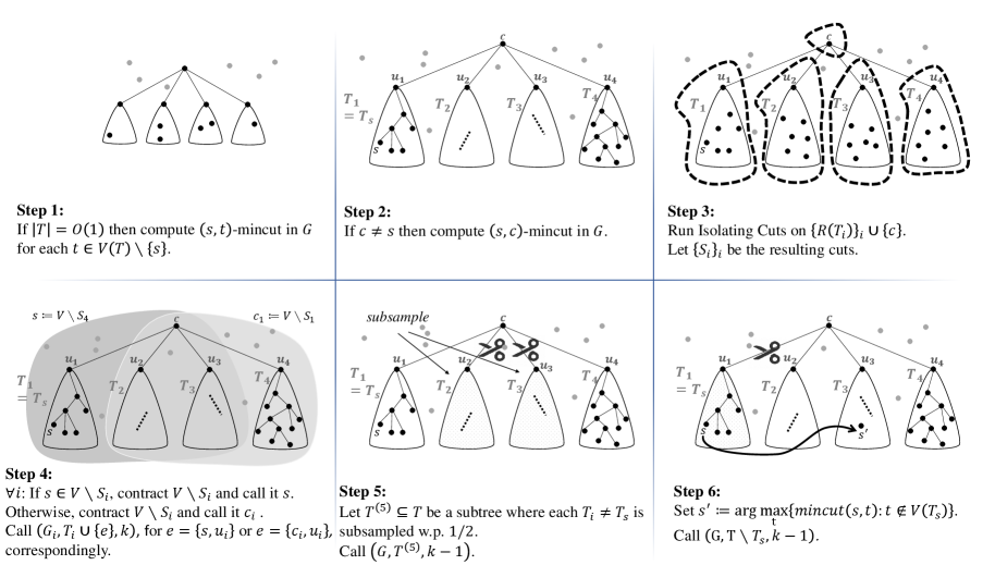
The SSMC Algorithm.
Having introduced the main tools, we are now ready to present our SSMC algorithm (see Figure 1). The input to the algorithm is a graph containing a specified vertex , a (guide) tree containing , and a positive integer . The algorithm is a recursive algorithm, and although the guide tree initially only contains vertices in , there will be additional vertices (not in ) that are introduced into the guide tree in subsequent recursive calls. To distinguish between these two types of vertices, we define as the subset of vertices of that are in , and call these real vertices. We call the vertices of that are not in fake vertices.
We extend the definition of -respecting (i.e., Definition 1.7) to fake vertices as follows:
Definition 2.4 (Generalized -respecting).
Let be a cut in . Let be a tree on (some subset of) vertices in as well as additional vertices not in . We say that -respects cut (and vice versa) if there exists a set of fake vertices such that contains at most edges with exactly one endpoint in ; we say that such edges are cut by .
We also note that even if all the vertices in are real vertices, may not be a subgraph of .
Recall that our goal is to obtain a value for every terminal such that if an -mincut -respects , then . We will actually compute for every real vertex ; clearly, this suffices since the input Steiner tree (i.e., at the top level of the recursion) spans all the vertices in .
The algorithm maintains estimates of the mincut values for all . The values are initialized to , and whenever we compute an -cut in the graph, we “update” by replacing with the value of the -cut if it is lower. Formally, we define .
We describe the algorithm below. The reader should use the illustration in Figure 1 as a visual description of each step of the algorithm.
-
1.
First, we describe a base case. If is less than some fixed constant, then we simply compute the -mincut in separately for each using max-flow calls, and run .
-
From now on, assume that is larger than some (large enough) constant.444For example, the constant is more than enough.
-
2.
Let be a centroid of the tree , defined in the following manner: is a (possibly fake) vertex in such that if we root at , then each subtree rooted at a child of has at most real vertices.555A centroid always exists by the following simple argument: take the (real or fake) vertex of of maximum depth whose subtree rooted at has at least real vertices. By construction, this vertex is a centroid of , and it can be found in time linear in the number of vertices in the tree using a simple dynamic program.
-
If and , then compute an )-mincut in (whose value is denoted ) using a max-flow call and run .
-
3.
Root at and let be the children of . For each , let be the subtree rooted at . Recall that denotes the set of real vertices in the respective subtrees for . (For technical reasons, we ignore subtrees that do not contain any real vertex.) Use 2.1 to compute minimum isolating cuts in with the following terminal sets: (1) for . (2) If , then we add an additional set . Note that irrespective of whether or not.
-
Let be the -mincut in obtained from 2.1. We ignore (if it exists) and proceed with the remaining sets for in the next step.
-
4.
For each , define as the graph with contracted to a single vertex. Now, there are two cases. In the first case, we have . Then, the contracted vertex for is labeled the new in graph . Correspondingly, define as the tree with an added edge (recall that is the root of ). In the second case, we have . Then, assign a new label to the contracted vertex for in . In this case, define as the tree with an added edge , and keep the identity of vertex unchanged since it is in . (Note that if , the only difference is that the second case does not happen for any .)
-
In both cases above, make recursive calls for all . Call for all where the recursive call returns the value for the variable . Furthermore, if , call for all where the recursive call returns the value for the variable .
-
If , then we terminate the algorithm at this point, so from now on, assume that .
-
5.
Sample each subtree independently with probability except the subtree containing (if it exists), which is sampled with probability . (If , then there is no subtree containing , and all subtrees are sampled with probability .) Let be the tree with all (vertices of) non-sampled subtrees deleted. Recursively call and update for all . (Note that denotes the set of real vertices in tree . Moreover, by the sampling procedure, is always in and hence, the recursion is valid.) Repeat this step for independent sampling trials.
-
6.
Execute this step only if , and let be the subtree from step (2) containing . Using Lemma 2.3, compute the value , as well as all vertices attaining this maximum. Update for all such , and arbitrarily select one such to be labeled . Let be the tree with (the vertices of) subtree removed. Recursively call where is treated as the new , and update for all .
2.1 Correctness
First, we show a standard (uncrossing) property of mincuts.
Lemma 2.5.
Let be a weighted, undirected graph with vertex subset . For any subsets and an -mincut of , there is an -mincut of satisfying .
Proof.
Consider any -mincut . We claim that is also an -mincut of . First, note that , so is an -cut. Since is an -mincut, we have
Combining the two inequalities gives . Now, since , we have . Since , it must be that . So, is an -cut. Since , it follows that is an -mincut, which completes the proof. ∎
Now, we proceed to establish correctness of the SSMC algorithm. Note that starts with the value , and every time we run , we have that is the value of some -cut in . Naturally, this would suggest that our estimate is always an upper bound on the true value . However, this is not immediately clear because the vertex may be relabeled in a recursive call from step (6). The lemma below shows that this relabeling is not an issue.
Lemma 2.6 (Upper bound).
For any instance and a vertex , the output value is at least .
Proof.
If is updated on Step (1) or Step (5), then we have because the updated value corresponds to a valid -cut. Suppose now that is updated on Step (2), and let be the subtree containing . By construction of , we either contract a set containing (namely, ) into a vertex labeled the new , or we contract a set not containing (namely, again) into a vertex (not labeled the new ). In both cases, any -cut of graph , with the contraction “reversed”, is a valid -cut in the original graph . It follows that the -mincut value 666 is the value of an -mincut in graph . in is at least the value in . By induction, the output of the recursive call is at least , as promised.
If is updated on Step (5), then since the graph remains unchanged, the value is also unchanged, and we have by induction. The most interesting case is when is updated on Step (6). Here, by the choice of , we have . Next, observe that holds because the -mincut is either an -cut or an -cut depending on whether is on the side of or the side of . Combining the two previous inequalities gives , and by induction, the output of the recursive call is at least , as promised. ∎
The lemma above establishes the condition of Theorem 1.10. It remains to show equality when is -respecting an -mincut, which we prove below.
Lemma 2.7 (Equality).
Consider an instance and a vertex such that there is an -mincut in that -respects . Then, the value computed by the algorithm equals w.h.p.
Proof.
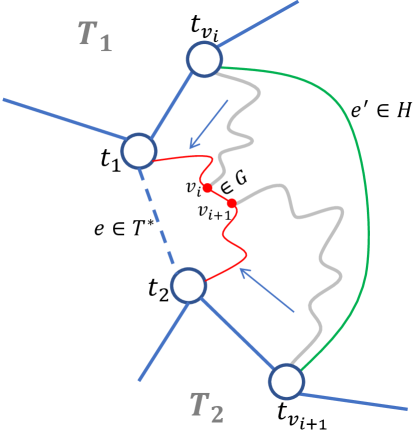
Consider an -mincut in that -respects . First, if the centroid is the vertex , then the mincut computation in Step (5) correctly recovers . Otherwise, let be the subtree containing . We have a few cases based on the locations of the edges in that cross the cut , which we call the cut edges. Note that there is at least one cut edge along the path in , and it is incident to (the vertices of) either or the subtree containing . (If and there is no subtree containing , then at least one cut edge must be incident on some vertex in .)
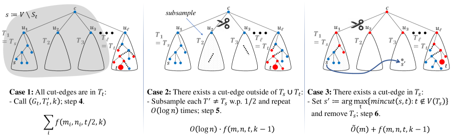
The first case (Case 1 in Figure 2) is that all the cut edges are incident to the vertices of a single subtree , which must be either or (if the latter exists). Then, there is a side of the -mincut whose vertices in are all in ; in other words, . Note that is an -mincut since if there were a smaller such cut, then that would also be a smaller -cut, which contradicts that is an -mincut. Also, by construction, is a -mincut. We now apply Lemma 2.5 on parameters , , , , and . The lemma implies that there is an -mincut , and this cut survives in the contracted graph . Since is an -cut of the same value as , we conclude that is also an -mincut. Finally, we argue that also -respects the tree in the recursive instance. By definition, since -respects , there exists a set of fake vertices such that contains at most edges cut by . Since and agree on vertices in , tree also contains at most edges cut by (it is the exact same set of edges). Define , and from , we observe that tree contains at most edges cut by (it is all edges from before, restricted to tree ). Furthermore, the new edge or added to is cut by if and only if the edge of is cut by . It follows that at most edges of are cut by . Thus, the lemma statement is satisfied on recursive call of Step (2), and the algorithm recovers w.h.p.
In the rest of the proof, we assume that the edges of cut by are incident to (the vertices of) at least two subtrees. Suppose first (Case 2 in Figure 2) that a cut edge is incident to some subtree that is not or (or only , if and does not exist). In each independent trial of Step (5), we sample but not with constant probability. In this case, since is discarded in the construction of , the -mincut -respects the resulting tree . Over independent trials, this happens w.h.p., and the algorithm correctly recovers w.h.p.
We are left with the case (Case 3 in Figure 2) that all edges of cut by are incident to subtrees and . Note that must exist since if and Case 2 does not happen, we would be in Case 1. Furthermore, , because otherwise, we would either be in Case 1 (if all cut edges are incident on ) or in Case 2 (if there is at least one cut edge incident on some ).
Since , we have , i.e., . If (where is as defined in Step (6)), then Step (6) sets correctly. Otherwise, we must have . In this case, we claim that the vertex (that has the property in Step (6) of the algorithm) satisfies . To prove this claim, we first observe that must appear on the -side of the -mincut . Otherwise, if is on the -side, then is an -cut of value , contradicting the guarantee . It follows that . Next, observe that must appear on the -side of the -mincut . Otherwise, if is on the -side, then is an -cut of value , contradicting the guarantee . It follows that , which proves the claim .
Consider again the -mincut . Since is on the -side of the -mincut , if we swap the locations of and in , then still -respects the modified tree, and the edges of the tree that cross the cut are the same (except that and swap places on the edges). In particular, the subtree with replaced by has at least one cut edge. By removing this modified subtree , we arrive at the tree in Step (6), and the -mincut must )-respect . So, the recursive call recovers w.h.p., which equals by the claim above.
This concludes all cases, and hence the proof of Lemma 2.7. ∎
2.2 Running Time
Lemma 2.8 (Running time).
For any fixed integer , the algorithm calls max-flow on instances of at most vertices and edges each, and a total of vertices and edges. Moreover, these max-flow calls dominate the running time.
We first bound the total number of vertices across all recursive instances, then use the same technique to also bound the total number of edges.
We use the following notation for any recursive call: and represents the number of vertices in including contracted vertices, i.e., vertices resulting from the contraction on Step (2) of any previous instance. (Since the original instance has no contracted vertex, the initial value of is just the number of vertices in the input graph.) The function represents an upper bound on the total number of vertices among all max-flow calls that occur, starting from a single input instance with parameters (and including max-flows called inside recursive instances).
Fix an instance with parameters . For each , let represent the number of vertices in , and let . Now observe that
-
1.
since the sets are disjoint by the guarantee of 2.1, and
-
2.
for each by the fact that is a centroid.
We now consider the individual steps of the recursive SSMC algorithm.
- 1.
-
2.
In step (2), the algorithm makes recursive calls on trees containing real vertices each, and graphs containing vertices each, so the total number of vertices in the max-flow calls in the recursion is at most .
-
3.
In step (5), the algorithm makes independent calls to an instance where decreases by . So, this step contributes at most .
- 4.
We may assume that is monotone non-decreasing in all three parameters, which gives us the recursive formula
We now claim that solves to for any constant , where the number of polylog terms depends on . For , the recursive formula solves to . This is because for all limits the recursive depth to .777Here, we have used the assumption that is larger than some constant, e.g. 10. And, since , the sum of in any recursive level is . For larger , note that if we assume that , then we also obtain , where the hides more logarithmic factors. The claim then follows by induction on . (Note that the polylogarithmic dependency on is .)
We now bound the total number of edges. We use the following notation in any recursive call: as earlier, and represents the number of vertices in including contracted vertices. In addition, represents plus the number of edges in not incident to a contracted vertex. (Since the original instance has no contracted vertex, the initial value of is just the number of vertices plus the number of edges in the input graph.) The function represents an upper bound on plus the total number of edges not incident to contracted vertices among all max-flow calls that occur, starting from a single input instance with parameters (and including max-flows called inside recursive instances). This then implies a bound on the total number of edges over all max-flow calls, including those incident to contracted vertices, by the following argument. Each recursive instance has at most contracted vertices, since each contraction in Step (2) decreases by a constant factor. So the total number of edges incident to contracted vertices is at most the total number of vertices times , which is at most . So from now on, we only focus on edges not incident to contracted vertices.
Fix an instance with parameters . For each , let represent the number of vertices in , let represent the number of edges in not incident to a contracted vertex, and let . Once again, observe that and for each . This time, we also have by the following explanation: 2.1 guarantees that the vertex sets are disjoint, and the edges of each not incident to a contracted vertex have both endpoints in , and are therefore disjoint over all . We may assume that is monotone non-decreasing in all four parameters, which gives us the recursive formula
Similar to the solution for , we now have that solves to for any constant by the same inductive argument. (Once again, the polylogarithmic dependency on is .)
Since the graph never increases in size throughout the recursion, each max-flow call is on a graph with at most as many vertices and edges as the original input graph. Finally, we claim that the max-flow calls dominate the running time of the algorithm. In particular, finding the centroid of on step (5) can be done in time in the size of the tree (see the footnote at step (5)), which is dominated by the single max-flow call on the same step. This finishes the proof of Lemma 2.8.
3 Constructing Guide Trees
In this section, we show how to obtain guide trees that prove Theorem 1.9. Our algorithm is based on the notion of a Steiner subgraph packing, as described next.
Definition 3.1.
Let be an undirected edge-weighted graph with a set of terminals . A subgraph of is said to be a -Steiner subgraph (or simply a Steiner subgraph if the terminal set is unambiguous from the context) if all the terminals are connected in . In this case, we also call a terminal-spanning subgraph of .
Definition 3.2.
A -Steiner-subgraph packing is a collection of -Steiner subgraphs , where each subgraph is assigned a value . If all are integral, we say that is an integral packing. Throughout, a packing is assumed to be fractional (which means that it does not have to be integral), unless specified otherwise. The value of the packing is the total value of all its Steiner subgraphs, denoted . We say that is feasible if
To understand this definition, think of as the “capacity” of ; then, this condition means that the total value of all Steiner subgraphs that “use” edge does not exceed its capacity . A Steiner-tree packing is a packing where each subgraph is a tree.
Denote by the maximum value of a feasible -Steiner-subgraph packing in . The next two lemmas show a close connection between Steiner-subgraph packing and -Steiner mincut , and that the former problem admits a -approximation algorithm.
Lemma 3.3.
For every graph with terminal set , we have .
Lemma 3.4.
There is a deterministic algorithm that, given , a graph , and a terminal set , returns a -Steiner-subgraph packing of value in time, and in the case of unweighted in time.
We prove Lemmas 3.3 and 3.4 in Sections 3.1 and 3.2, respectively. Assuming these lemmas, we immediately obtain the following.
Corollary 3.5.
There is a deterministic algorithm that, given and a graph with edges and terminal set , returns a -Steiner subgraph packing of value in time, and in the case of unweighted in time.
Algorithm for constructing guide trees.
Given Corollary 3.5, we can now prove Theorem 1.9.
Proof of Theorem 1.9.
Fix (or another sufficiently small ). The construction of guide trees is described in Algorithm 1. To analyze this algorithm, let be the packing computed in line 1. Consider , and let be a minimum -cut in . Denote by the total edge-weight of this cut in , and by the total edge-weight of the cut in between these same vertices.
Consider first an unweighted input . Then, the computation in line 1 is applied to . By combining Corollary 3.5 and the promise in the single source terminal mincuts problem (1.5) that , 888For a graph , denotes the value of an -mincut in , and recall that is the value of a -Steiner mincut in . we get that
| (1) |
If the input graph is weighted, then the bound in (1) applies to the cut-sparsifier of , and we get that
| (2) |
We remark that now the packing contains subgraphs of the sparsifier and not of , but it will not pose any issue.
In both cases we have the weaker inequality
| (3) |
Let be the set of edges in the cut in (depending on the case, is either or the sparsifier). Let be the subset of all Steiner subgraphs whose intersection with is at most edges, and let be the event that no subgraph from is sampled in line 1. Then
| (4) |
Similarly to Karger’s paper [Kar00], define to be one less than the number of edges of that crosses the cut , and observe that is always a non-negative integer (because is connected in ). Since is a packing, every edge of appears in at most one subgraph of , and consequently,
Observe that for a random drawn as in line 1,
where the last inequality is by (3). By Markov’s inequality,
Observe that , and so by plugging into we get that . Finally, by a union bound we have that with high probability, for every , at least one of the subgraphs that are sampled in line 1 of the algorithm -respects the cut ,999Strictly speaking, Definition 1.7 defines -respecting only relative to a tree , but the same wording extends immediately to any graph (not necessarily a tree). and thus at least one of the trees reported by the algorithm -respects . Furthermore, since the cut in has the exact same bipartition of as the -mincut in , the reported tree mentioned above -respects also the -mincut in (recall that Definition 1.7 refers to a cut as a bipartition of ).
Finally, computing a Steiner tree of a Steiner subgraph in Line 1 only takes linear time, and so the running time is dominated by line 1 and thus it is bounded by for weighted graphs and by for unweighted graphs, and by fixing a small , we can write these as and , respectively. This concludes the proof of Theorem 1.9. ∎
3.1 Steiner-Subgraph Packing vs Steiner Mincut
In this section, we prove 3.3, i.e., that .
We start with the second inequality , which is easier. Let be a -Steiner-subgraph packing, and let be a Steiner min-cut of . Then for every Steiner subgraph , by definition .101010For any graph , the set of edges in the cut is denoted . By the feasibility of , for every we have . Putting these together, we conclude that
To establish the first inequality , we need to show that one can always pack into Steiner subgraphs of total value (at least) . This packing bound actually follows from more general theorems of Bang-Jensen et al. [BFJ95] and Bhalgat et al. [BHKP07, BCH+08], but we give a simple self-contained proof here.
First note that we can assume, only for sake of analysis, that the graph is an unweighted multi-graph (by replacing each edge by parallel edges of unit weight) and that every vertex has an even degree (by appropriate scaling). (In what follows, we will obtain an integral packing but undoing the scaling step possibly converts it into a fractional packing.)
We use the following classic result due to Mader [Mad78].
Theorem 3.6.
Let be an undirected unweighted multi-graph where every vertex has an even degree.111111In the original theorem of Mader, the only restriction is that the degree of cannot be equal to 3. But, for our purposes, it suffices to assume that every vertex has even degree. Then, there exists a pair of edges and incident on that can be split off, i.e., replaced by their shortcut edge , while preserving the edge connectivity for all pairs of vertices .
By applying Theorem 3.6 repeatedly on edges incident on , we can isolate the vertex . Iterating further, we can isolate any subset of vertices while preserving the pairwise edge connectivities of all the remaining vertices. We thus isolate all the non-terminal vertices, and then delete these isolated vertices to obtain a graph only on the terminal vertices . Observe that edges in represent edge-disjoint paths in . We also claim that the global edge connectivity of is at least . Indeed, the global edge connectivity of equals the minimum of all its pairwise edge connectivities, which are all preserved from , and it is clear that in all pairwise edge connectivities are at least .
Next, we shall use the following classic theorem of Nash-Williams [NW61] and Tutte [Tut61] to pack edge-disjoint spanning trees in .
Theorem 3.7.
Let be an undirected unweighted multi-graph with global edge connectivity . Then, contains at least edge-disjoint spanning trees.
Now we apply this theorem to our graph , to pack in it (at least) edge-disjoint spanning trees, and then replace each edge in these spanning trees of by its corresponding path in . These paths are edge-disjoint as well, hence the corresponding subgraphs are edge-disjoint in . This yields a set of (at least) edge-disjoint -spanning subgraphs in , which completes the proof of 3.3.
3.2 -approximate Steiner-Subgraph Packing
In this section, we provide a -approximation algorithm for fractionally packing Steiner subgraphs, proving 3.4. The technique is a standard application of the width-independent multiplicative weight update (MWU) framework [GK07, Fle00, AHK12]. We provide the proofs for completeness, following closely the presentation from [CS21].
We start by describing, in Section 3.2.1, an algorithm based on the multiplicative weight update framework, and we bound its number of iterations, also called “augmentations”. Then, in Section 3.2.2, we show how to implement these augmentations efficiently by using either a static -approximation algorithm by Mehlhorn [Meh88], or in unweighted graphs, by using a decremental -approximation algorithm from Theorem 4.1.
3.2.1 Algorithm Based on Multiplicative Weight Update
Let the input be an edge-weighted graph with vertices, edges, and terminal set . Denote by the set of all -Steiner subgraphs. The algorithm maintains , which we refer to as edge lengths.121212Multiplicative weight update algorithms usually maintain “weights” on edges of the input graph. We use here instead the terminology of edge lengths, because already has edge weights (that can be viewed as capacities). The total length of a subgraph is defined as . A -Steiner subgraph is said to have -approximate minimum -length if its length satisfies . Our algorithm below for packing Steiner subgraphs assumes access to a procedure that computes a -approximate minimum -length Steiner subgraph.
Lemma 3.8.
The scaled-down packing computed by Algorithm 2 is feasible.
Proof.
Given a packing , if we define the “flow” (or load) on an edge as , then we need to show that for all . (This terminology highlights the analogy with packing flow paths and thinking of as the capacity of .) Consider the computation of before scaling it down in line 2. Whenever an iteration adds some into the packing (in line 2), it effectively increases the flow additively by for some , and the corresponding length is increased multiplicatively by (in line 2). Observe that initially and at the end (because prior to the last iteration ), thus over the course of the execution, grows multiplicatively by at most , implying that at the end of the execution, . Hence, scaling down by factor in line 2 makes this packing feasible. ∎
We call each iteration in the while loop of Algorithm 2 an augmentation and say that an edge participates in the augmentation if is contained in the Steiner subgraph of that iteration (in line 2). The next lemma is used to bound the total running time.
Lemma 3.9.
-
(a).
If is unweighted, then each edge participates in at most augmentations.
-
(b).
There are at most augmentations.
Proof.
(a) Fix . In every augmentation, because is unweighted. So whenever participates in an augmentation, is increased by factor . Since initially and at the end, can participate in at most augmentations.
(b) By the choice of in each augmentation, at least one edge has its length increased by factor . For every edge , initially and at the end , and thus the total number of augmentations is bounded by . ∎
Lemma 3.10.
The scaled-down packing is a -approximate -Steiner subgraph packing.
Proof.
We first write an LP for the -Steiner subgraph packing problem and its dual LP, using our notation .
Denote , and let be the length of the minimum -length -Steiner subgraph. Let be the edge-length function after executions of the while loop (and by convention refers to just before entering the loop). For brevity, denote and . We also denote by the Steiner subgraph found in the -th iteration and by the value of (before scaling down). Observe that
Since is a -approximate minimum -length -Steiner subgraph,
Observe that the optimal value of the dual LP can be written as , and thus
Let be the index of the last iteration, then . Since , we get
Taking a logarithm from both sides, and denoting , we get
| (5) |
Notice that is exactly the value of before scaling down in line 2. By 3.8, the scaled-down packing is a feasible solution for the primal , and thus by weak duality . Thus, to prove that it achieves -approximation, it suffices to show that . And indeed, using (5) and the fact that , i.e., , we have
where the last inequality holds because and . ∎
3.2.2 Efficient Implementation
In this section, we complete the proofs of 3.4 by providing an efficient implementation of Algorithm 2 from Section 3.2.1.
-time Algorithms for General Graphs.
In line 2 of Algorithm 2, we invoke the algorithm of Mehlhorn [Meh88] for -approximation of the minimum-length Steiner tree (it clearly approximates also the minimum-length Steiner subgraph, because an optimal Steiner subgraph is always a tree). Each invocation runs in time , which subsumes the time complexity of other steps in a single iteration of the while loop. There are iterations by 3.9(a), hence the total running time is . The packing produced as output is a -approximate solution by 3.10.
-time Algorithms for Unweighted Graphs.
In unweighted graphs, we obtain an almost-linear time by invoking the data structure from Theorem 4.1, which is a dynamic algorithm that maintains a graph under edge-weight increases and can report a -approximate minimum-length Steiner subgraph. Then in line 2 of Algorithm 2, we query to obtain a graph , and in line 2 we instruct to update the edge lengths. The packing produced as output is again an -approximate solution by 3.10, and it only remains to analyze the total running time.
A small technical issue is that maintains a graph whose edge lengths are integers in the range . Our edge lengths lie in the range , which can be scaled to the range . Each update to is further rounded upwards to the next integer, and thus we can use . The rounding increases edge lengths multiplicatively by at most , and thus each reported subgraph achieves -approximation with respect to the unrounded lengths. We can prevent the rounding error from accumulating, by maintaining a table of the exact lengths of each edge (separately from ), and using this non-rounded value when computing the edge’s new length in line 2.
The overall running time is dominated by the time spent by updates and queries to the data structure . By 3.9(a), each edge participates in at most augmentations and thus appears in at most different Steiner subgraphs . As each iteration updates only the lengths of edges in its subgraph , the total number of edge-length updates, over the entire execution, is at most . By Theorem 4.1, the total update time of is . Lastly, returns each Steiner subgraph in time , and therefore the total time of all queries is . Thus, the overall running time is .
4 Decremental -approximate Minimum Steiner Subgraphs
The goal of this section is to establish an algorithm for maintaining a -approximate minimum Steiner subgraph with amortized time per weight-increase update, and output-sensitive query time. In this paper, the main application of this algorithm is in proving Theorem 1.9: fractionally packing -Steiner-subgraphs in an unweighted graph with -Steiner mincut in almost-linear time. More specifically, this result gets used inside the MWU framework (Lemma 3.4). However, it can also be viewed as a result of independent interest: obtaining an almost-optimal algorithm for a classic problem in the decremental (weight-increase) setting. To be consistent with Section 3.2.1 we refer to the edge-weights as lengths. A key feature of this new algorithm is that it is deterministic, and therefore works in an adaptive-adversary setting (such as MWU).
Theorem 4.1 (Decremental Approximate Minimum Steiner Subgraph).
For any constant , there is a deterministic data-structure that maintains a graph with terminals under a sequence of updates (edge-length-increase only) in total time, and can, at any time, produce a -approximate minimum -length -Steiner subgraph of in time where is the number of edges in the subgraph it outputs.
At a high-level, there are two distinct steps for establishing this result:
-
1.
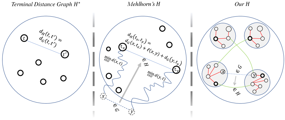
A reduction to decremental Single-Source Shortest Paths (SSSP). It is well-known that a -approximation for Steiner Tree can be obtained by computing the Minimum Spanning Tree (MST) of a helper graph . This helper graph is simply the complete distance graph of the terminals, and (naively) requires time to compute. The MST of then gets expanded into a Steiner subgraph of . Mehlhorn’s algorithm achieves a -approximation in time by further reducing the problem to an SSSP computation, by seeking the MST of a slightly different helper graph . At a high-level, our plan is to design a dynamic version of Mehlhorn’s algorithm.
-
2.
An almost-optimal decremental algorithm for -SSSP. The challenge with the above reduction is in the difficult task of maintaining the SSSP information that is required to construct the helper graph while the input graph is changing. Roughly speaking, we succeed in doing that, while paying an additional factor, due to a recent decremental -SSSP deterministic algorithm by Bernstein, Gutenberg, and Saranurak [BGS22] with time per update.
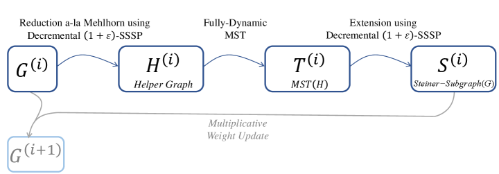
Thus, the plan is as follows. Let be the graph after the update. Using a decremental -SSSP algorithm we maintain a helper graph . Then, using a fully-dynamic MST algorithm we maintain the MST of . Whenever there is a query, we output a Steiner subgraph of by querying for the MST of and expanding it into . Notably, whereas is obtained from in a decremental fashion, i.e. only via increasing edge-lengths, the updates to the helper graph can be both decremental and incremental. As a result, we need to maintain the MST in a fully-dynamic setting, which can be done in update time with a deterministic algorithm [HdLT01]. This is schematically described in Figure 3.
Realizing this plan, however, involves several lower-level challenges. First of all, the construction of the helper graph from Mehlhorn’s algorithm needs to be modified in order to prevent the number of changes to from being much larger than the number of changes to . (Otherwise, each edge update in could result in edge changes in .) This is presented in Section 4.2. Second, the new construction of a helper graph has slightly different properties than Mehlhorn’s which we state and analyze next in Section 4.1. And finally, the reduction requires additional features from the -SSSP data-structure that were not explicitly stated in previous work. We explain how they can be achieved (with minor modifications) in the discussion below Lemma 4.10.
4.1 The Helper Graph
We begin by describing what properties the helper graph should have, and by proving that they suffice for the MST of to yield a -approximate -Steiner tree for . The algorithm for dynamically maintaining a helper graph with these properties is discussed later on. Note that we will have a helper graph of in each step , but the properties we describe in this section are indifferent to the step and to the fact that we are in a dynamic environment; therefore we will drop the superscript in this subsection.
The starting point of both our helper graph and Mehlhorn’s original construction is the well-known fact that an MST of the complete distance graph of the terminals is a -approximation to the Steiner tree.
Lemma 4.2 ([HR92, TM80, KMB81, Ple81]).
Let be a graph with terminals , and let be the distance graph of the terminals, i.e. . Then, the MST of has length at most times the minimum -Steiner tree of .
The issue with this helper graph is in the complexity of computing (and maintaining) it. Mehlhorn’s fast algorithm is based on the observation that a different helper graph, that can be viewed as a proxy towards , suffices to get a -approximation. The exact property of a helper graph that Mehlhorn’s algorithm is based on is stated in the next lemma. (The analysis of our helper graph will not use this Lemma; we only include it for context.)
Lemma 4.3 ([Meh88]).
Let be a graph with terminals , and let be a weighted graph such that for each edge there exists an edge , where and are the closest terminals to and (respectively), of length . Then, the MST of has length at most times the minimum -Steiner tree of .
Notice that a pair of vertices in may have many parallel edges between them with different lengths. (See Figure 4 for an illustration.)
As an intermediate step towards defining the properties of our actual helper graph, we consider the following approximate version of Mehlhorn’s definition. We say that is a -closest terminal to iff for all .
Lemma 4.4.
Let be a graph with terminals , and let be a graph such that: (1) for each vertex there is a unique terminal assigned to , where is a -closest terminal to , and (2) for each edge there exists an edge of length . Then, the MST of has length at most times the minimum -Steiner tree of .
Proof.
Let be an MST of the ideal helper graph (the complete distance graph of the terminals). We will prove that there exists an MST of our helper graph with length . Then by Lemma 4.2 we get that the MST of has length at most times the minimum -Steiner tree of .
We describe a process that modifies by replacing its edges with edges from while keeping it a terminal spanning tree and while only increasing its length by (see Figure 5).
Specifically, each edge gets replaced by an edge of length . We will do this replacement as long as there is an edge in that is not in , or is in but has a different length than it does in .
Let be such an edge, and let be a shortest path from to in with total length . The removal of from disconnects the tree into two components, call them and . Let be such that but . Such an must exist because and .
Consider the edge that follows from the edge by the assumptions on the helper graph . Replacing with keeps a terminal spanning tree. It only remains to bound the difference in lengths:
Since is a -closest terminal to we know that and similarly . Therefore,
∎
Our actual helper graph, described next, differs from Mehlhorn’s not only in the fact that it is approximate, but more importantly, it is a graph on the entire vertex set rather than just the terminals. This is done for efficiency; the (admittedly vague) intuition is as follows. Updating each edge of after each update to is too costly because the closest (or even the -closest) terminal to a vertex might change very frequently. But one can observe that most of these frequent changes are not important for the MST; there is usually a parallel edge that was not affected and whose length is within of the new edges that we would want to add. Figuring out which changes in are important and which are not does not seem tractable. Instead, our new idea is to make the update only in a helper graph that is, on the one hand, much closer to than to Mehlhorn’s helper graph (and therefore doesn’t change too frequently), and on the other hand, has the same MST up to as Mehlhorn’s. In other words, the idea is to let the MST algorithm do the work of figuring out which edges are relevant.
The properties that our actual helper graph will satisfy are described in the following lemma. In words, each terminal has a disjoint component in of vertices that can be reached from with distance (due to edges of length zero in ). The components morally represent the approximate Voronoi cells of the terminals. And instead of demanding that each edge of the original graph be represented by an edge between the two corresponding terminals in the helper graph, we only demand that there be some edge between the two corresponding components (where need not be terminals).
Lemma 4.5.
Let be a graph with terminals , and let be a weighted graph satisfying the following properties:
-
•
for each vertex there is a unique terminal such that ,
-
•
for each edge there exists an edge with and , where and are -closest terminals to and in (respectively), of length .
Then, the MST of has length at most times the minimum -Steiner tree of .
Proof.
For each terminal let be the component of vertices at distance zero to . By the assumption on , the sets form a partition of . Let be the graph obtained from by contracting each into a single vertex. It immediately follows that is a helper graph that satisfies requirements of Lemma 4.4 above, and therefore the MST of has length at most times the minimum -Steiner tree of . But any MST of can be expanded into an MST of with the same length, by taking a zero-length spanning tree for each component ; the shortest path tree rooted at is such a tree. ∎
4.2 Maintaining the Helper Graph Dynamically: A Reduction to SSSP
The main technical result towards proving Theorem 4.1 is an algorithm for maintaining a helper graph with the properties required by Lemma 4.5.
Lemma 4.6.
Given a graph with terminal set and a sequence of length-increase updates, it is possible to maintain a helper graph satisfying the properties in Lemma 4.5 with a deterministic algorithm such that:
-
•
The total time is , and
-
•
The recourse, i.e. number of edge-length changes to throughout the sequence, is .
-
•
Given an MST of of total length it is possible to produce a -Steiner subgraph of of total length , in time where is the number of edges in the subgraph.
This lemma is proved in the next sections. But first, let us explain how Theorem 4.1 follows from it.
Proof of Theorem 4.1.
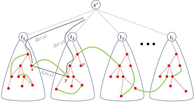
Let be the input graph that is undergoing a sequence of length-increase updates; let be the graph after the update. We use the algorithm in Lemma 4.6 to maintain a helper graph as changes; let be the helper graph after the update. We use the fully-dynamic MST algorithm by Holm et al. [HdLT01], with as the input, to (explicitly) maintain an MST of as changes. If after the update, there is a query asking for a -Steiner subgraph for , we first inspect the MST data-structure to obtain an MST of . We use the algorithm in Lemma 4.6 again to expand the MST into a -Steiner subgraph of . If the total length of the MST is then the total length of the Steiner subgraph is , and therefore, since the helper graph satisfies the properties of Lemma 4.5, we get that is a -minimum -Steiner subgraph for .
The running time for maintaining the helper graph is . To bound the running time of the MST algorithm we first need to bound the number of updates we make to (not ) because is the input graph to the MST algorithm. This number of updates is exactly the recourse and it is bounded by . The MST algorithm [HdLT01] has amortized update time (and is deterministic) and therefore it can support this number of updates in a total of time as well. Finally, the time to produce the -Steiner subgraph is where is the number of edges in the subgraph, as required by Theorem 4.1. ∎
4.2.1 The Basic Construction
In order to understand our final construction of the helper graph , it is helpful to first see a simplified version that works assuming an SSSP data-structure with (slightly) stronger properties than currently achievable.
Let us first briefly overview how a decremental SSSP data-structure works, to clarify the context of some of the notation below. Naturally, the idea is to maintain a shortest-path tree rooted at the source . For efficiency, it is desirable that the tree’s depth be small. For this reason, the data-structures (e.g. [HKN14, BGS22]) typically use a hopset: by adding a set of edges to the graph, it is guaranteed that there exist a path from to any that is -shortest-path and that only uses edges; namely, it has only hops. A hopset-edge typically has a length that corresponds to the shortest path distance between its endpoints, and therefore the distance in the new graph is never shorter than the original distance. The data-structure then maintains an approximate shortest-path tree on the graph with the hopset, of depth , which can be done efficiently. The distances that it reports are exactly the distances in this tree.
Proposition 4.7.
Suppose that there is a deterministic data-structure that given a graph and a single-source , that undergoes a sequence of edge-length-increase updates, and supports the following operations in total time:
-
•
Explicitly maintains an estimate for each , such that . In particular, can report after each update, all vertices such that increased by a factor (since the last time was reported).
-
•
Explicitly maintains a tree rooted at , such that for all . An edge of the tree is either from or from a set of hopset-edges . In particular, can report after each update, all edges that are added or removed from .
Moreover, it holds that each hopset-edge of length is associated with a -path in of length . And that the number of times an edge may appear on a single root-to-leaf path in , either as an edge or as an edge on the path of a hopset-edge , is . Additionally, the data-structure supports the following query:
-
•
Given a hopset-edge and an integer , can return the first (or last) edges of in time .
Then Lemma 4.6 holds.
The main difference between the requirements of Proposition 4.7 and the features of the existing -SSSP algorithm is simply that the data-structure explicitly maintains trees instead of one, and the tree is only guaranteed to approximate to within the distances when they are in the range (for some ). Another minor gap is that the hopsets use auxiliary vertices, in addition to the shortcut edges. These gaps will be handled in the next subsection. For now, let us see how to obtain Proposition 4.7.
Proof of Proposition 4.7.
We start off with a trick similar to the way Mehlhorn’s algorithm reduces the problem of computing the closest terminal to each vertex (i.e. the Voronoi cell of each terminal) to an SSSP problem. Let be the graph obtained from by adding a super-source that is connected with edges of length to all terminals (see Figure 6).
Consequently, for any vertex , , and moreover belongs to the subtree rooted at in the SSSP-tree rooted at . Note that this can be achieved without really using edges of length by simply contracting all terminals into one vertex and calling it .131313The description below assumes we do add the zero-length edges. In the full construction in the next subsection we do in fact need to use the contractions, and so the arguments differ in minor ways. We will run the -SSSP data-structure in the statement on with as the source. Note that it is trivial to transform the length-increase sequence of updates to into a sequence of length-increase updates on . Let and be the tree and estimates maintained by the data-structure.
Maintaining a helper graph
The helper graph is defined based on , and as follows. Note that the vertex set of is the same as ’s; in our full construction (in the next subsection) there will be additional vertices. There are two kinds of edges in :
-
•
Green edges: for each edge we add an edge to with length
A green edge gets updated whenever: (1) the length gets updated and is more than times the value used in the current , or (2) the data-structure reports that or is increased by a factor.
-
•
Red edges: for each edge we add an edge of length to .141414The zero-length edges between and each terminal in are exempted, since does not exist in . A red edge gets updated whenever the tree changes. If an edge is removed from the tree, the red edge is removed (i.e. the length is increased from to infinity),151515Notably, these are the only incremental updates that we do. and if a new edge is added to the tree we add an edge of length zero to .
The recourse of the helper graph
The data-structure will not only maintain the helper graph described above, but it will also feed it into a dynamic MST algorithm and explicitly maintain an MST of . For this to be efficient, we must argue that the total number of updates we make to is small. The running time of the data-structure is upper bounded by , and since it stores the tree explicitly, this is also an upper bound on the total number of changes to . Whenever a red edge is updated it is because the corresponding edge was updated in ; this can happen times. A green edge is updated either when the corresponding edge in has its length increase by at least a factor, or when or increase by . Since the lengths and estimates are upper bounded by , they can only increase by a factor times. Each time an estimate increases we would update edges in . Thus, the total number of updates to the green edges is . It follows that the running time and total number of updates to is .
The properties of the helper graph
Next, let us prove that satisfies the two properties in Lemma 4.5. For that, it is helpful to establish the following claims.
Claim 4.8.
In the tree the root has all of the terminals in as children.
Proof.
Suppose for contradiction that is in the subtree of terminal . Then it must follow that because all edges that are not adjacent to in have non-zero length. On the other hand, , contradicting the fact that . ∎
The first of the two properties in Lemma 4.5 now follows. In the tree , each vertex appears in the subtree of exactly one terminal and, due to the red edges, has distance . For all other terminals the path from to must use a green edge of length .
Claim 4.9.
For all , . Moreover, if is in the subtree of terminal then is a -closest terminal to .
Proof.
The first part follows from the fact that , and the guarantee on the estimates. For the second part note that ; thus, is a -closest terminal to . ∎
To prove the second property, let be an edge in ; we will show that the green edge satisfies the requirement.161616That is, we prove the property with and . This will not be the case in the full construction in the next subsection. Let and be such that and . By the above claim, we know that and are -closest terminals to and (respectively) in . Finally, we can upper bound the length of the green edge in by
Expanding an MST of into a -Steiner subgraph of
By the above we know that the length of an MST of is a -approximation to the minimum length of a Steiner subgraph of . So if our goal was only to maintain an approximation to the length of a Steiner-Tree, we would just use the length of a given MST of and be done. Alas, for our applications the data-structure must return the subgraph itself, which is more complicated. The process of (efficiently) expanding an MST into a Steiner subgraph is as follows.
For a terminal we define ’s component (or subtree or Voronoi cell) to be the set of vertices that are connected by red edges to . Pick an arbitrary terminal as a starting point. We will construct a Steiner Subgraph by starting from and iteratively adding paths (in ) to it. Let be the set of terminals that are spanned by ; initially . In each step, we pick an arbitrary green edge of the MST that has an endpoint in one of the components of the terminals in . Let be such an edge, and let be the two terminals such that are in their components (respectively). First, note that such an edge must exist as long as (or else the MST does not span the entire graph). Second, note that but (otherwise there would be a cycle in the MST). We would like to add to : (1) a path from to , (2) the edge , and (3) a path from to . This would connect to and therefore add to . And we would like to have that the total length of (1) + (2) + (3) is at most . Ignoring certain subtle details, this can be done by observing that and the distances in come from paths in . Namely, we can scan the path from to in and, whenever we encounter an edge from we simply add it to , while if we encounter an edge we ask the data-structure to expand it into the path and add to . If we do this, the total length of the final Steiner Subgraph will be exactly .
The subtle issue with the above is that the total running time for outputting a Steiner Subgraph with edges may not be even though every time the data-structure reports an edge it only costs time. Indeed, if edges are reported throughout the above process, we only spend time, but due to edges being repeated many times, the number of edges that we finally output could be much smaller than .171717While the total length from the repetitions is still within our budget of , the MWU framework does not allow us to spend more than time on an edge we output, even if it is being repeated many times in the output. To resolve this issue we use a more careful process that uses the ability of the data-structure to list only the first or last edges on a path at cost only ; it turns out that if we see an edge that we have already seen, we can stop expanding .
In more details, the step for expanding a green edge is as follows. We start from (rather than ) and scan the tree down to . When we see an edge we check if it is already in :
-
•
If it is not in we add it to a set of edges that will be added to at the end of the step.
-
•
If happens to already be in , then we stop, add all edges in to , and finish the step of edge . This makes sense because the edges in form a path from to and all of is connected to , so we have accomplished the goal of connecting to (at a potentially cheaper length than ).
And when we see an edge we do the following for each : ask the data-structure to report the first (closest to ) edges of , call them , and check if they are already in :
-
•
If none of them are in we add them to the set of edges that will be added to at the end of the step.
-
•
Otherwise, let be the first (closest to ) reported edge that is already in . We stop the step, add all edges in to , and finish the step of edge . The edges in form a path from to and therefore to , so we are done.
If we reach without stopping, we continue on to the edge . Again, we check if it is already in ; if not we add it to , if it is, we stop and add all of into . Similarly, after reaching we continue by scanning the tree up to . When encountering an edge from or we do the exact steps above to decide if we should add it to or stop. If we reach the without stopping, we add all of into and finish the step.
We claim that the total time for the above process is where is the number of distinct edges that end up in . Consider the step corresponding to an edge , and let be the first edge on the corresponding path from to (the one closest to ) that is already in before the step. Let be the edges that come before on the path, and let be the number of distinct edges among them; note that the step ends up adding new edges to and our goal is to bound its running time by . By the assumption on the data-structure, each edge can appear only times on a root-to-leaf path in , and therefore . Due to the repeated doubling of in the above process, each edge might get reported an additional times, and more importantly, the number of edges that come after on the path and that the data-structure reports (but do not end up in ) is . Therefore, the total time can be upper bounded by .
∎
4.2.2 The Full Construction
We are now ready to present our actual construction. The proof is heavily based on the proof of the simpler construction above.
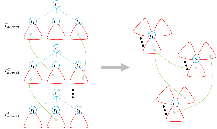
Lemma 4.10.
Suppose that for any constant , there is a deterministic data-structure that given a graph and a source , that undergoes a sequence of edge-length-increase updates of length , and supports the following operations in total time. There is a parameter such that, for each :
-
•
Explicitly maintains an estimate for each , such that and if then . In particular, can report after each update, all vertices such that increased.
-
•
Explicitly maintains a graph where is not a subgraph of and contains all vertices of but also a set of auxiliary vertices, which forms an independent set in . For any pair of regular vertices , if has length or there is an auxiliary vertex such that is a -path of length , then there is an associated -path in of length between and . Although is not a simple path, each edge in may appear at most times in .
-
•
Explicitly maintains a tree rooted at in of depth , such that for all . In particular, can report after each update, all edges that are added or removed from .
Additionally, the data-structure supports the following query:
-
•
For each path in , given an integer , can return the first (or last) edges of in time .
Then Lemma 4.6 holds.
A data-structure with the above requirements indeed exists by the recent work of Bernstein et al. [BGS22]. Since this exact formulation was not explicitly stated in [BGS22], let us point out how to obtain it. In Section III.5 of [BGS22], there are distance scales of the data structures where . For each scale , the objects in Lemma 4.6, such as the estimates for all , are maintained by the data structure described in Sections II.5 and III.3 of [BGS22]. is called an emulator in Definition II.5.2 in [BGS22]. A vertex corresponds to a core (see Definition II.2.8 of [BGS22]). The tree is the Monotone Even-Shiloach tree maintained by as described in Section II.5.2.
The only guarantee which was implicit in [BGS22] is the last bullet point about returning the first/last edges in the path in time. This guarantee follows by inspecting Algorithm 7 of [BGS22]. When the algorithm needs to report the whole path , it does so by recursively querying the data structure starting from the largest distance scale to the smallest distance scale. More precisely, the path is represented by a hierarchical tree of depth whose leaves correspond to edges of and internal vertices correspond to subpaths of . Each internal vertex has children ordered according to the ordering of the edges in the path. Now, when we query only for the first edges in the path, the algorithm would resemble the situation when we have a balanced binary search tree and we want to list the first leaves of this tree. For our setting, the tree has depth and each vertex has children. By recursively querying the multi-level data structures in this way, we will obtain the first edges of the path in time.
Proof.
The proof follows along the lines of the proof of Proposition 4.7 but with a few modifications. As before, we apply the data-structure on the graph that is obtained from by adding a super-source that represents all terminals in . Rather than adding zero-length edges between each and we contract all terminals into a single vertex and call it . Note that each edge in can be traced back to an edge for some . Let and be the trees and estimates maintained by the data-structure, where .
Maintaining a helper graph
The helper graph is defined based on , the trees and estimates as follows. For each vertex in we create copies in . A terminal vertex however only has one copy . Moreover, we add all auxiliary vertices in for all to . There are two kinds of edges in :
-
•
Green edges: for each edge we add edges to , for all , and set their length to
A green edge gets updated whenever: (1) the length gets updated and is more than times the value used in the current , or (2) the data-structure reports that or increased by a factor.
-
•
Red edges: for each edge for some we add an edge of length to . If one of or is , suppose w.l.o.g. that it is , then we trace the edge back to an edge and we add an edge of length to . A red edge gets updated whenever the tree changes. If an edge is removed from the tree, the red edge is removed (i.e. the length is increased from to infinity),181818As before, these are the only incremental update that we do. and if a new edge is added to the tree we add an edge of length zero to .
(See Figure 7 for an illustration.)
The recourse of the helper graph
The upper bound on the total running time and recourse of maintaining follows exactly as in the simpler construction above, with the exception that there is an additional factor due to the number of times an edge is copied.
The properties of the helper graph
Next, let us prove that satisfies the two properties in Lemma 4.5.
For the first property, consider any vertex , for some , and our goal is to prove that there is exactly one terminal such that . First, observe that the only red edges that are adjacent to a vertex come from edges in the tree . Let be the first edge on the path from to in . This edge can be traced back to an edge where . Due to the red edges, we will have . On the other hand, since is a tree, there cannot be any other path from to and consequently there will not be any other terminal with a red path to (via edges from . The only other way that could potentially reach with a red path is if could reach via edges from some other and then use the red path from to . However, by construction, any red path between two terminals implies a loop in one of the trees – a contradiction.
To prove the second property, let be an edge in , and let be such that and . Consequently, and . We will show that the green edge satisfies the requirement. Let and be such that and . By an argument similar to Claim 4.9 from before, we know that and are -closest terminals to and (respectively) in . This is because , and similarly . Finally, we can upper bound the length of the green edge in by
Expanding an MST of into a -Steiner subgraph of
To conclude the proof we point out that the process of expanding an MST of into a Steiner Subgraph of can be carried out in exactly the same way as in the previous subsection, with the minor detail that we have to get rid of the auxiliary vertices if they are in the MST. By assumption, there are no edges between them, so we can simply make the expansion on two-paths in the MST (that skip over auxiliary vertices) rather than edges. This expansion of an edge or two-path of length into a path in of length up to introduces a factor to the total length of the Steiner subgraph (that we did not have in the simple construction). ∎
5 Conclusion
In this paper, we broke the longstanding cubic barrier for the GHtree and APMF problems in general, weighted graphs. All previous improvements since 1961, were either corollaries of speed-ups in (single-pair) max-flow algorithms, or were limited to special graph classes. Assuming the APSP Conjecture, a cornerstone of fine-grained complexity, our result disproves the belief that computing max-flows is at least as hard as computing shortest-paths.
Our algorithm has a running time of which is nearly-optimal for APMF if all max-flow values must be returned. For GHtree in unweighted graphs, our techniques yield an improved running time of . In fact, a succinct representation of all-pairs max-flows can be produced in the time of calls to a (single-pair) max-flow algorithm.
It is an interesting open question as to whether our techniques can be extended to obtain an -time GHtree algorithm for weighted graphs as well. In particular, the most significant challenge is to design a new dynamic Steiner tree subroutine (analogous to the one in Section 4) that can be used for packing Steiner trees in weighted graphs in almost-linear time.
References
- [ACK20] A. Abboud, V. Cohen-Addad, and P. N. Klein. New hardness results for planar graph problems in p and an algorithm for sparsest cut. In K. Makarychev, Y. Makarychev, M. Tulsiani, G. Kamath, and J. Chuzhoy, editors, Proccedings of the 52nd Annual ACM SIGACT Symposium on Theory of Computing, STOC 2020, Chicago, IL, USA, June 22-26, 2020, pages 996–1009. ACM, 2020. Available from: https://doi.org/10.1145/3357713.3384310, doi:10.1145/3357713.3384310.
- [ACZ98] S. R. Arikati, S. Chaudhuri, and C. D. Zaroliagis. All-pairs min-cut in sparse networks. J. Algorithms, 29(1):82–110, 1998. doi:10.1006/jagm.1998.0961.
- [AD16] A. Abboud and S. Dahlgaard. Popular conjectures as a barrier for dynamic planar graph algorithms. In I. Dinur, editor, IEEE 57th Annual Symposium on Foundations of Computer Science, FOCS 2016, 9-11 October 2016, Hyatt Regency, New Brunswick, New Jersey, USA, pages 477–486. IEEE Computer Society, 2016. Available from: https://doi.org/10.1109/FOCS.2016.58, doi:10.1109/FOCS.2016.58.
- [AGI+19] A. Abboud, L. Georgiadis, G. F. Italiano, R. Krauthgamer, N. Parotsidis, O. Trabelsi, P. Uznanski, and D. Wolleb-Graf. Faster Algorithms for All-Pairs Bounded Min-Cuts. In 46th International Colloquium on Automata, Languages, and Programming (ICALP 2019), volume 132, pages 7:1–7:15, 2019. doi:10.4230/LIPIcs.ICALP.2019.7.
- [AGW15] A. Abboud, F. Grandoni, and V. V. Williams. Subcubic equivalences between graph centrality problems, APSP and diameter. In P. Indyk, editor, Proceedings of the Twenty-Sixth Annual ACM-SIAM Symposium on Discrete Algorithms, SODA 2015, San Diego, CA, USA, January 4-6, 2015, pages 1681–1697. SIAM, 2015. Available from: https://doi.org/10.1137/1.9781611973730.112, doi:10.1137/1.9781611973730.112.
- [AHK12] S. Arora, E. Hazan, and S. Kale. The multiplicative weights update method: a meta-algorithm and applications. Theory of Computing, 8(1):121–164, 2012.
- [AIS+16] T. Akiba, Y. Iwata, Y. Sameshima, N. Mizuno, and Y. Yano. Cut tree construction from massive graphs. In 2016 IEEE 16th International Conference on Data Mining (ICDM), pages 775–780. IEEE, 2016.
- [AKT20] A. Abboud, R. Krauthgamer, and O. Trabelsi. Cut-equivalent trees are optimal for min-cut queries. In 61st IEEE Annual Symposium on Foundations of Computer Science, FOCS 2020, pages 105–118, 2020. doi:10.1109/FOCS46700.2020.00019.
- [AKT21a] A. Abboud, R. Krauthgamer, and O. Trabelsi. APMF APSP? Gomory-Hu tree for unweighted graphs in almost-quadratic time. Accepted to FOCS’21, 2021. arXiv:2106.02981.
- [AKT21b] A. Abboud, R. Krauthgamer, and O. Trabelsi. New algorithms and lower bounds for all-pairs max-flow in undirected graphs. Theory of Computing, 17(5):1–27, 2021. doi:10.4086/toc.2021.v017a005.
- [AKT21c] A. Abboud, R. Krauthgamer, and O. Trabelsi. Subcubic algorithms for gomory–hu tree in unweighted graphs. In Proceedings of the 53rd Annual ACM SIGACT Symposium on Theory of Computing, pages 1725–1737, 2021. doi:10.1145/3406325.3451073.
- [AKT22] A. Abboud, R. Krauthgamer, and O. Trabelsi. Friendly cut sparsifiers and faster Gomory-Hu trees. Accepted to SODA’22, 2022. arXiv:2110.15891.
- [AMO93] R. Ahuja, T. Magnanti, and J. Orlin. Network Flows. Prentice Hall, 1993.
- [AV20] N. Anari and V. V. Vazirani. Planar graph perfect matching is in NC. Journal of the ACM, 67(4):1–34, 2020.
- [AVY15] A. Abboud, V. Vassilevska Williams, and H. Yu. Matching triangles and basing hardness on an extremely popular conjecture. In Proc. of 47th STOC, pages 41–50, 2015.
- [AW14] A. Abboud and V. V. Williams. Popular conjectures imply strong lower bounds for dynamic problems. In 55th IEEE Annual Symposium on Foundations of Computer Science, FOCS 2014, pages 434–443, 2014. doi:10.1109/FOCS.2014.53.
- [AW21] J. Alman and V. V. Williams. A refined laser method and faster matrix multiplication. In Proceedings of the 2021 ACM-SIAM Symposium on Discrete Algorithms, SODA 2021, pages 522–539, 2021. doi:10.1137/1.9781611976465.32.
- [BBDF06] D. Barth, P. Berthomé, M. Diallo, and A. Ferreira. Revisiting parametric multi-terminal problems: Maximum flows, minimum cuts and cut-tree computations. Discrete Optimization, 3(3):195–205, 2006.
- [BCH+08] A. Bhalgat, R. Cole, R. Hariharan, T. Kavitha, and D. Panigrahi. Efficient algorithms for Steiner edge connectivity computationand Gomory-Hu tree construction for unweighted graphs. Unpublished full version of [BHKP07], 2008. Available from: http://hariharan-ramesh.com/papers/gohu.pdf.
- [BDT16] A. Backurs, N. Dikkala, and C. Tzamos. Tight hardness results for maximum weight rectangles. In I. Chatzigiannakis, M. Mitzenmacher, Y. Rabani, and D. Sangiorgi, editors, 43rd International Colloquium on Automata, Languages, and Programming, ICALP 2016, July 11-15, 2016, Rome, Italy, volume 55 of LIPIcs, pages 81:1–81:13. Schloss Dagstuhl - Leibniz-Zentrum für Informatik, 2016. Available from: https://doi.org/10.4230/LIPIcs.ICALP.2016.81, doi:10.4230/LIPIcs.ICALP.2016.81.
- [BENW16] G. Borradaile, D. Eppstein, A. Nayyeri, and C. Wulff-Nilsen. All-pairs minimum cuts in near-linear time for surface-embedded graphs. In 32nd International Symposium on Computational Geometry, volume 51 of SoCG ’16, pages 22:1–22:16, 2016. doi:10.4230/LIPIcs.SoCG.2016.22.
- [BFJ95] J. Bang-Jensen, A. Frank, and B. Jackson. Preserving and increasing local edge-connectivity in mixed graphs. SIAM J. Discret. Math., 8(2):155–178, 1995. doi:10.1137/S0036142993226983.
- [BGK20] S. Baswana, S. Gupta, and T. Knollmann. Mincut sensitivity data structures for the insertion of an edge. In 28th Annual European Symposium on Algorithms (ESA 2020), 2020.
- [BGMW20] K. Bringmann, P. Gawrychowski, S. Mozes, and O. Weimann. Tree edit distance cannot be computed in strongly subcubic time (unless apsp can). ACM Transactions on Algorithms (TALG), 16(4):1–22, 2020.
- [BGS22] A. Bernstein, M. P. Gutenberg, and T. Saranurak. Deterministic decremental sssp and approximate min-cost flow in almost-linear time. In 2021 IEEE 62nd Annual Symposium on Foundations of Computer Science (FOCS), pages 1000–1008. IEEE, 2022.
- [BHKP07] A. Bhalgat, R. Hariharan, T. Kavitha, and D. Panigrahi. An Gomory-Hu tree construction algorithm for unweighted graphs. In 39th Annual ACM Symposium on Theory of Computing, STOC’07, pages 605–614, 2007. doi:10.1145/1250790.1250879.
- [BK15] A. A. Benczúr and D. R. Karger. Randomized approximation schemes for cuts and flows in capacitated graphs. SIAM J. Comput., 44(2):290–319, 2015. doi:10.1137/070705970.
- [BSW15] G. Borradaile, P. Sankowski, and C. Wulff-Nilsen. Min -cut oracle for planar graphs with near-linear preprocessing time. ACM Trans. Algorithms, 11(3), 2015. doi:10.1145/2684068.
- [BT17] A. Backurs and C. Tzamos. Improving viterbi is hard: Better runtimes imply faster clique algorithms. In International Conference on Machine Learning, pages 311–321. PMLR, 2017.
- [CCPS97] W. Cook, W. Cunningham, W. Pulleybank, and A. Schrijver. Combinatorial Optimization. Wiley, 1997.
- [CKL+22] L. Chen, R. Kyng, Y. P. Liu, R. Peng, M. P. Gutenberg, and S. Sachdeva. Maximum flow and minimum-cost flow in almost-linear time. CoRR, abs/2203.00671, 2022. Available from: https://doi.org/10.48550/arXiv.2203.00671, arXiv:2203.00671, doi:10.48550/arXiv.2203.00671.
- [CLP22] R. Cen, J. Li, and D. Panigrahi. Augmenting edge connectivity via isolating cuts. In Proceedings of the 2021 ACM-SIAM Symposium on Discrete Algorithms, SODA 2022, 2022.
- [CMWW19] M. Cygan, M. Mucha, K. Wegrzycki, and M. Włodarczyk. On problems equivalent to (min,+)-convolution. ACM Transactions on Algorithms (TALG), 15(1):1–25, 2019.
- [CQ21] C. Chekuri and K. Quanrud. Isolating cuts,(bi-) submodularity, and faster algorithms for connectivity. In 48th International Colloquium on Automata, Languages, and Programming (ICALP 2021). Schloss Dagstuhl-Leibniz-Zentrum für Informatik, 2021.
- [CS21] J. Chuzhoy and T. Saranurak. Deterministic algorithms for decremental shortest paths via layered core decomposition. In Proceedings of the 2021 ACM-SIAM Symposium on Discrete Algorithms (SODA), pages 2478–2496. SIAM, 2021.
- [Dij59] E. W. Dijkstra. A note on two problems in connexion with graphs. Numerische mathematik, 1(1):269–271, 1959.
- [Elm64] S. E. Elmaghraby. Sensitivity analysis of multiterminal flow networks. Operations Research, 12(5):680–688, 1964.
- [Fle00] L. K. Fleischer. Approximating fractional multicommodity flow independent of the number of commodities. SIAM Journal on Discrete Mathematics, 13(4):505–520, 2000.
- [GH61] R. E. Gomory and T. C. Hu. Multi-terminal network flows. Journal of the Society for Industrial and Applied Mathematics, 9:551–570, 1961. Available from: http://www.jstor.org/stable/2098881.
- [GK07] N. Garg and J. Könemann. Faster and simpler algorithms for multicommodity flow and other fractional packing problems. SIAM Journal on Computing, 37(2):630–652, 2007.
- [GMW21] P. Gawrychowski, S. Mozes, and O. Weimann. Planar negative k-cycle. In D. Marx, editor, Proceedings of the 2021 ACM-SIAM Symposium on Discrete Algorithms, SODA 2021, Virtual Conference, January 10 - 13, 2021, pages 2717–2724. SIAM, 2021. Available from: https://doi.org/10.1137/1.9781611976465.161, doi:10.1137/1.9781611976465.161.
- [GR98] A. V. Goldberg and S. Rao. Beyond the flow decomposition barrier. J. ACM, 45(5):783–797, 1998. doi:10.1145/290179.290181.
- [GT01] A. V. Goldberg and K. Tsioutsiouliklis. Cut tree algorithms: an experimental study. Journal of Algorithms, 38(1):51–83, 2001.
- [Gus90] D. Gusfield. Very simple methods for all pairs network flow analysis. SIAM Journal on Computing, 19(1):143–155, 1990.
- [HdLT01] J. Holm, K. de Lichtenberg, and M. Thorup. Poly-logarithmic deterministic fully-dynamic algorithms for connectivity, minimum spanning tree, 2-edge, and biconnectivity. Journal of the ACM (JACM), 48(4):723–760, 2001. doi:10.1145/502090.502095.
- [HKN14] M. Henzinger, S. Krinninger, and D. Nanongkai. Decremental single-source shortest paths on undirected graphs in near-linear total update time. In 2014 IEEE 55th Annual Symposium on Foundations of Computer Science, pages 146–155. IEEE, 2014.
- [HL07] R. Hassin and A. Levin. Flow trees for vertex-capacitated networks. Discrete Appl. Math., 155(4):572–578, 2007. doi:10.1016/j.dam.2006.08.012.
- [HR92] F. K. Hwang and D. S. Richards. Steiner tree problems. Networks, 22(1):55–89, 1992. doi:10.1002/net.3230220105.
- [Hu74] T. C. Hu. Optimum communication spanning trees. SIAM Journal on Computing, 3(3):188–195, 1974. doi:10.1137/0203015.
- [HW13] T. Hartmann and D. Wagner. Dynamic Gomory–Hu tree construction–fast and simple. arXiv preprint arXiv:1310.0178, 2013.
- [Jel63] F. Jelinek. On the maximum number of different entries in the terminal capacity matrix of oriented communication nets. IEEE Transactions on Circuit Theory, 10(2):307–308, 1963. doi:10.1109/TCT.1963.1082149.
- [Kar00] D. R. Karger. Minimum cuts in near-linear time. Journal of the ACM, 47(1):46–76, 2000.
- [KL15] D. R. Karger and M. S. Levine. Fast augmenting paths by random sampling from residual graphs. SIAM J. Comput., 44(2):320–339, 2015. doi:10.1137/070705994.
- [KMB81] L. T. Kou, G. Markowsky, and L. Berman. A fast algorithm for steiner trees. Acta Informatica, 15:141–145, 1981. Available from: https://doi.org/10.1007/BF00288961, doi:10.1007/BF00288961.
- [KT18] R. Krauthgamer and O. Trabelsi. Conditional lower bounds for all-pairs max-flow. ACM Trans. Algorithms, 14(4):42:1–42:15, 2018. doi:10.1145/3212510.
- [KV12] B. Korte and J. Vygen. Combinatorial optimization, volume 2. Springer, 2012.
- [Li21] J. Li. Preconditioning and Locality in Algorithm Design. PhD thesis, Carnegie Mellon University, 2021.
- [LNP+21] J. Li, D. Nanongkai, D. Panigrahi, T. Saranurak, and S. Yingchareonthawornchai. Vertex connectivity in poly-logarithmic max-flows. In Proceedings of the 53rd Annual ACM SIGACT Symposium on Theory of Computing, pages 317–329, 2021.
- [LP20] J. Li and D. Panigrahi. Deterministic min-cut in poly-logarithmic max-flows. In 61st IEEE Annual Symposium on Foundations of Computer Science, FOCS 2020, pages 85–92, 2020. doi:10.1109/FOCS46700.2020.00017.
- [LP21] J. Li and D. Panigrahi. Approximate Gomory-Hu tree is faster than max-flows. In STOC ’21: 53rd Annual ACM SIGACT Symposium on Theory of Computing, pages 1738–1748. ACM, 2021. doi:10.1145/3406325.3451112.
- [LPS21] J. Li, D. Panigrahi, and T. Saranurak. A nearly optimal all-pairs min-cuts algorithm in simple graphs. Accepted to FOCS’21, 2021. arXiv:2106.02233.
- [Mad78] W. Mader. A reduction method for edge-connectivity in graphs. In B. Bollobás, editor, Advances in Graph Theory, volume 3 of Annals of Discrete Mathematics, pages 145–164. Elsevier, 1978. doi:https://doi.org/10.1016/S0167-5060(08)70504-1.
- [May62] W. Mayeda. On oriented communication nets. IRE Transactions on Circuit Theory, 9(3):261–267, 1962. doi:10.1109/TCT.1962.1086912.
- [Meh88] K. Mehlhorn. A faster approximation algorithm for the steiner problem in graphs. Information Processing Letters, 27(3):125–128, 1988.
- [MN21] S. Mukhopadhyay and D. Nanongkai. A note on isolating cut lemma for submodular function minimization. arXiv preprint arXiv:2103.15724, 2021.
- [NS18] G. Naves and F. B. Shepherd. When do Gomory-Hu subtrees exist? CoRR, 2018. Available from: http://arxiv.org/abs/1807.07331.
- [NW61] C. S. A. Nash-Williams. Edge-Disjoint Spanning Trees of Finite Graphs. Journal of the London Mathematical Society, s1-36(1):445–450, 01 1961. doi:10.1112/jlms/s1-36.1.445.
- [Pan16] D. Panigrahi. Gomory-Hu trees. In M.-Y. Kao, editor, Encyclopedia of Algorithms, pages 858–861. Springer New York, 2016. doi:10.1007/978-1-4939-2864-4_168.
- [Ple81] J. Plesník. The complexity of designing a network with minimum diameter. Networks, 11(1):77–85, 1981. Available from: https://doi.org/10.1002/net.3230110110, doi:10.1002/net.3230110110.
- [PQ80] J.-C. Picard and M. Queyranne. On the structure of all minimum cuts in a network and applications. In Combinatorial Optimization II, pages 8–16. Springer, 1980.
- [PR82] M. W. Padberg and M. R. Rao. Odd minimum cut-sets and -matchings. Mathematics of Operations Research, 7(1):67–80, 1982.
- [RZ04] L. Roditty and U. Zwick. On dynamic shortest paths problems. In European Symposium on Algorithms, pages 580–591. Springer, 2004.
- [Sah15] B. Saha. Language edit distance and maximum likelihood parsing of stochastic grammars: Faster algorithms and connection to fundamental graph problems. In V. Guruswami, editor, IEEE 56th Annual Symposium on Foundations of Computer Science, FOCS 2015, Berkeley, CA, USA, 17-20 October, 2015, pages 118–135. IEEE Computer Society, 2015. Available from: https://doi.org/10.1109/FOCS.2015.17, doi:10.1109/FOCS.2015.17.
- [Sch03] A. Schrijver. Combinatorial Optimization. Springer, 2003.
- [Sei95] R. Seidel. On the all-pairs-shortest-path problem in unweighted undirected graphs. Journal of computer and system sciences, 51(3):400–403, 1995.
- [TM80] H. Takahashi and A. Matsuyama. An approximate solution for the Steiner problem in graphs. Math. Japon., 24(6):573–577, 1979/80.
- [Tut61] W. T. Tutte. On the Problem of Decomposing a Graph into n Connected Factors. Journal of the London Mathematical Society, s1-36(1):221–230, 01 1961. doi:10.1112/jlms/s1-36.1.221.
- [WL93] Z. Wu and R. Leahy. An optimal graph theoretic approach to data clustering: Theory and its application to image segmentation. IEEE transactions on pattern analysis and machine intelligence, 15(11):1101–1113, 1993.
- [WW18] V. V. Williams and R. R. Williams. Subcubic equivalences between path, matrix, and triangle problems. J. ACM, 65(5):27:1–27:38, 2018. doi:10.1145/3186893.
- [Zha21] T. Zhang. Gomory-Hu trees in quadratic time. arXiv preprint arXiv:2112.01042, 2021.
- [Zha22] T. Zhang. Faster Cut-Equivalent Trees in Simple Graphs. In 49th International Colloquium on Automata, Languages, and Programming (ICALP 2022), volume 229 of Leibniz International Proceedings in Informatics (LIPIcs), pages 109:1–109:18, Dagstuhl, Germany, 2022. arXiv:2106.03305, doi:10.4230/LIPIcs.ICALP.2022.109.
Appendix A Reduction to Single-Source Terminal Mincuts Given a Promise
Before giving the formal reduction, let us give a high-level description. The original Gomory-Hu algorithm is a reduction to max-flow calls. At a high-level, it starts with all vertices in one super-vertex and recursively bi-partitions , until contains only one vertex. In any recursive step, the input to the algorithm is the set (called terminals) and a graph that is formed from contracting sets of vertices in the input graph in previous recursive steps. In the current step, the algorithm picks an arbitrary pair of vertices and computes an -mincut in . Then, it creates two recursive subproblems, where in each subproblem, one side of the -mincut cut is retained uncontracted and the other side is contracted into a single vertex. The new in a subproblem comprises the vertices in on the uncontracted side.
The contractions serve to enforce consistency between the cuts, so that we end up with a tree structure of cuts. But, recent work has shown that these contractions also help with efficiency. Suppose that instead of an arbitrary pair (which can lead to unbalanced cuts and large recursive depth), we split using single-source mincuts from a random pivot to all other terminals . It turns out that with sufficiently high probability, the cuts from the random pivot to many other terminals only contain at most (say) -fraction of the vertices in , and splitting according to all these cuts (instead of into two) leads to recursion whose depth is bounded by .
Effectively, this gives a reduction from GHtree to the single-source mincuts problem, with only a multiplicative overhead in the running time. The random-pivot idea was first used by Bhalgat et al. [BHKP07] but the first general reduction to single-source mincuts is by Abboud et al. [AKT20]. We use a refined reduction that has two additional features: (1) the algorithm (for the single-source problem) only needs to return the values of the cuts rather than the cuts themselves (and in fact, it is given estimates and only needs to decide if they are correct), and (2) the mincut values between any pair of terminals in the graph are guaranteed to be within a (say) -factor from each other (the so called “promise”). The first restriction only serves to simplify our new algorithm, while the second is more important for our new ideas to work. This is encapsulated in Lemma 1.6 which we prove below.
As discussed in the overview, we first remove the “promise” condition from the single source terminal mincuts problem (1.5). To be precise, we first formally define the single source terminal mincuts problem without the promise.
Problem A.1 (Single-Source Terminal Mincuts (without Promise)).
The input is a graph , a terminal set and a source terminal . The goal is to determine the value of for each terminal .
We also require the approximate single-source mincuts algorithm of [LP21], stated below, which we use as a black box.
Theorem A.2 (Theorem 1.7 of [LP21]).
Let be a graph, let , and let be a constant. There is an algorithm that outputs, for each vertex , a -approximation of , and runs in time plus calls to max-flow on -vertex, -edge graphs, where is the ratio of maximum to minimum edge weights.
We now present the reduction that removes the promise.
Lemma A.3.
There is a randomized algorithm for the unconditional Single-Source Terminal Mincuts problem (A.1) that makes calls to the promise version of the Single-Source Terminal Mincuts problem (1.5) on graphs with a total of vertices and edges. Outside of these calls, the algorithm takes time plus calls to max-flow on -vertex, -edge graphs.
Proof.
Call Theorem A.2 with ; note that since the input graph is integer-weighted with maximum weight . Let be the computed approximations, which satisfy . For each integer , let be all vertices with . Note that is nonempty for only many integers , since must be in the range .
We first claim that for each , the terminal set satisfies the promise of 1.5, namely that for all , we have . To prove this claim, note that for each ,
so all values are in the range . Moreover, we must have since the Steiner mincut of is an -mincut for some . It follows that by the choice , concluding the claim.
For the remainder of this section, we reduce Gomory-Hu tree to the unconditional Single-Source Terminal Mincuts (A.1). The reduction is virtually identical to Section 4.5 of [Li21], and we include it for the sake of completeness.
Theorem A.4.
There is a randomized algorithm that outputs a Gomory-Hu tree of a weighted, undirected graph w.h.p. It makes calls to the unconditional Single-Source Terminal Mincuts problem (A.1) on graphs with a total of vertices and edges. It also calls max-flow on graphs with a total of vertices and edges, and runs for time outside of these calls.
The precise Gomory-Hu tree algorithm that proves Theorem A.4 is described in Algorithm LABEL:ghtree a few pages down.
A.1 Additional Preliminaries
For this section, we need to formally define a generalization of Gomory-Hu trees called Gomory-Hu Steiner trees that are more amenable to our recursive structure.
Definition A.5 (Gomory-Hu Steiner tree).
Given a graph and a set of terminals , the Gomory-Hu Steiner tree is a weighted tree on the vertices , together with a function , such that
-
•
For all , consider the minimum-weight edge on the unique – path in . Let be the vertices of the connected component of containing . Then, the set is an -mincut, and its value is .
In our analysis, we use the notion of a minimal mincut and a rooted minimal Gomory-Hu tree. We define these next.
Definition A.6 (Minimal -mincut).
A minimal -mincut is an -mincut whose side containing is vertex-minimal.
Definition A.7 (Rooted minimal Gomory-Hu Steiner tree).
Given a graph and a set of terminals , a rooted minimal Gomory-Hu Steiner tree is a Gomory-Hu Steiner tree on , rooted at some vertex , with the following additional property:
-
For all , consider the minimum-weight edge on the unique path in ; if there are multiple minimum weight edges, let denote the one that is closest to . Let be the vertices of the connected component of containing . Then, is a minimal -mincut, and its value is .
The following theorem establishes the existence of a rooted minimal Gomory-Hu Steiner tree rooted at any given vertex.
Theorem A.8.
For any graph , terminals , and root , there exists a rooted minimal Gomory-Hu Steiner tree rooted at .
Proof.
Let be a small enough weight, and let be the graph with an additional edge of weight added for each . (If the edge already exists in , then increase its weight by instead.) If is small enough, then for all and , if is an -mincut in , then is an -mincut in .
Let be a Gomory-Hu Steiner tree for . We claim that it is essentially a minimal Gomory-Hu Steiner tree for , except that its edge weights need to be recomputed as mincuts in and not . More formally, let be the tree with the following edge re-weighting: for each edge in , take a connected component of and reset the edge weight of to be and not . We now claim that is a minimal Steiner Gomory-Hu tree for .
We first show that is a Gomory-Hu Steiner tree for . Fix , let be the minimum-weight edge on the – path in , and let be the vertices of the connected component of containing . Since is a Gomory-Hu Steiner tree for , we have that is an -mincut in . If is small enough, then by our argument from before, is also an -mincut in . By our edge re-weighting of , the edge has the correct weight. Moreover, is the minimum-weight edge on the – path in , since a smaller weight edge would contradict the fact that is an -mincut.
We now show the additional property that makes a minimal Gomory-Hu Steiner tree. Fix , and let and be defined as in , i.e., is the minimum-weight edge on the path that is closest to , and is the vertices of the connected component of containing . Since is a Gomory-Hu Steiner tree for , we have that is an -mincut of value . Suppose for contradiction that is not a minimal -mincut. Then, there exists such that is also an -mincut. By construction of , and . We have and , so . In other words, is not an -mincut in , contradicting the fact that is a Gomory-Hu Steiner tree for . Therefore, property is satisfied, concluding the proof. ∎
A.2 A Single Recursive Step
Before we present Algorithm LABEL:ghtree, we first consider the subprocedure LABEL:ghtreestep that it uses on each recursive step.
-
1.
Initialize and
-
2.
For all from to do:
-
(a)
Call the Isolating Cuts Lemma (2.1) on the singleton sets for , obtaining disjoint sets (the minimal -mincut) for each .
-
(b)
Call A.1 on graph and source .
-
(c)
Let be the union of over all satisfying and
-
(d)
subsample of where each vertex in is sampled independently with probability , and is sampled with probability
-
(a)
-
3.
Return the largest set and the corresponding sets over all satisfying the conditions in line 2c
Let be the union of the sets as defined in Algorithm LABEL:ghtreestep. Let be all vertices for which there exists an -mincut whose side has at most vertices in . We now claim that covers a large fraction of vertices in in expectation.
Lemma A.9.
.
Proof.
Consider a rooted minimal Steiner Gomory-Hu tree of on terminals rooted at , which exists by Theorem A.8. For each vertex , let be defined as the child vertex of the lowest weight edge on the path from to in . If there are multiple lowest weight edges, choose the one with the maximum depth.
For each vertex , consider the subtree rooted at , define to be the vertices in the subtree, and define as the number of vertices in the subtree. We say that a vertex is active if for . In addition, if , then we say that hits all of the vertices in (including itself); see Figure 8. In particular, in order for to hit any other vertex, it must be active. For completeness, we say that any vertex in is not active and does not hit any vertex.
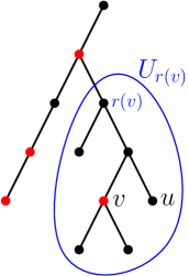
To prove that , we will show that
-
(a)
each vertex that is hit is in ,
-
(b)
the total number of pairs for which hits is at least in expectation for some small enough constant , and
-
(c)
each vertex is hit by at most vertices.
For (a), consider the vertex that hits . By definition, for , we have , so is a -cut. By the definition of , we have that is a -mincut. On the other hand, we have that is a -mincut, so in particular, it is a -cut. It follows that and are both -mincuts and -mincuts, and . Since is a minimal Gomory-Hu Steiner tree, we must have . Since is the minimal -mincut, it is also the minimal -mincut, so . It follows that . Since is the minimal -mincut and , we must have , so in particular, . Therefore, the vertex satisfies all the conditions of line 2c. Moreover, since , vertex is added to in the set .
For (b), for , we have with probability exactly , and with probability , no other vertex in joins . Therefore, is active with probability . Conditioned on being active, it hits exactly many vertices. It follows that hits vertices in expectation.
For (c), since the isolating cuts over are disjoint for each , each vertex is hit at most once on each iteration . Since there are many iterations, the property follows.
Finally, we show why properties (a) to (c) imply . By property (b), the number of times some vertex hits another vertex is in expectation. Since each vertex is hit at most times by property (c), there are at least vertices hit in expectation, all of which are included in by property (a). ∎
The corollary below immediately follows. Note that the sets output by the algorithm are disjoint, which we require in the recursive GH tree algorithm.
Corollary A.10.
The largest set returned by LABEL:ghtreestep satisfies .
A.3 The Gomory-Hu Tree Algorithm
The Gomory-Hu tree algorithm is presented in LABEL:ghtree, which uses LABEL:ghtreestep as a subprocedure on each recursive step.
Correctness.
Algorithm LABEL:ghtree has the same recursive structure as Gomory and Hu’s original algorithm, except that it computes multiple mincuts on each step. Therefore, correctness of the algorithm follows similarly to their analysis. For completeness, we include it below.
-
1.
uniformly random vertex in
-
2.
Call to obtain and the sets (so that )
-
3.
For each set do: Construct recursive graphs and apply recursion
-
(a)
Let be the graph with vertices contracted to a single vertex are disjoint
-
(b)
Let
-
(c)
If , then recursively set
-
(a)
-
4.
Let be the graph with (disjoint) vertex sets contracted to single vertices for all
-
5.
Let
-
6.
If , then recursively set
-
7.
Combine and into according to LABEL:combine
-
8.
Return
Lemma A.11.
Algorithm LABEL:ghtree outputs a Gomory-Hu Steiner tree.
To prove Lemma A.11, we first introduce a helper lemma.
Lemma A.12.
For any distinct vertices , we have . The same holds with and replaced by and for any .
Proof.
Since is a contraction of , we have . To show the reverse inequality, fix any -mincut in , and let be one side of the mincut. We show that for each , either or . Assuming this, the cut stays intact when the sets are contracted to form , so .
Consider any , and suppose first that . Then, is still a -cut, and is still a -cut. By the submodularity of cuts,
In particular, must be a minimum -cut. Since is the minimal -mincut, it follows that , or equivalently, .
Suppose now that . In this case, we can swap and , and swap and , and repeat the above argument to get .
The argument for and is identical, and we skip the details. ∎
Proof (Lemma A.11)..
We apply induction on . By induction, the recursive outputs and are Gomory-Hu Steiner trees. By definition, this means that for all and the minimum-weight edge on the – path in , letting be the vertices of the connected component of containing , we have that is an -mincut in with value is . Define as the vertices of the connected component of containing . By construction of (lines 1 and 2), the set is simply with the vertex replaced by in the case that . Since is simply with all vertices contracted to , we conclude that . By Lemma A.12, we have are equal, so is an -mincut in . In other words, the Gomory-Hu Steiner tree condition for is satisfied for all . A similar argument handles the case for some .
There are two remaining cases: and , and and for distinct . Suppose first that and . By considering which sides and lie on the -mincut, we have
We now case on which of the three mincut values is greater than or equal to.
-
1.
If , then since is a -mincut that is also an -cut, we have . By construction, the edge of weight is on the path in . There cannot be edges on the path in of smaller weight, since each edge corresponds to a -cut in of the same weight. Therefore, is the minimum-weight edge on the – path in .
-
2.
Suppose now that . The minimum-weight edge on the path in has weight . This edge cannot be on the path in , since otherwise, we would obtain a -cut of value in , which becomes a -cut in after expanding the contracted vertex ; this contradicts our assumption that . It follows that is on the path in which, by construction, is also on the path in . Once again, the path cannot contain an edge of smaller weight.
-
3.
The final case is symmetric to case 2, except we argue on and instead of and .
Suppose now that and for distinct . By considering which sides lie on the -mincut, we have
We now case on which of the four mincut values is greater than or equal to.
-
1.
If or , then the argument is the same as case 1 above.
-
2.
If or , then the argument is the same as case 2 above.
This concludes all cases, and hence the proof. ∎
Running time.
We now bound the running time of LABEL:ghtree.
Lemma A.13.
W.h.p., the algorithm LABEL:ghtree has maximum recursion depth .
Proof.
By construction, each recursive instance has . We use the following lemma from [AKT20].
Lemma A.14.
Suppose the source vertex is chosen uniformly at random. Then, .
By Corollary A.10 and Lemma A.14, over the randomness of and LABEL:ghtreestep, we have
so the recursive instance satisfies . Therefore, each recursive branch either has at most half the vertices in , or has at most a fraction in expectation. It follows that w.h.p., all branches terminate by recursive calls. ∎
Lemma A.15.
For a weighted graph and terminals , takes time plus calls to max-flow on instances with a total of vertices and edges.
Proof.
For a given recursion level, consider the instances across that level. By construction, the terminals partition . Moreover, the total number of vertices over all is at most since each branch creates new vertices and there are at most branches.
To bound the total number of edges, define a parent vertex in an instance as a vertex resulting from either (1) contracting in some previous recursive call, or (2) contracting a component containing a parent vertex in some previous recursive call. There are at most parent vertices: at most can be created by (1) since each call decreases by a constant factor, and (2) cannot increase the number of parent vertices. Therefore, the total number of edges adjacent to parent vertices is at most times the number of vertices. Since there are vertices in a given recursion level, the total number of edges adjacent to parent vertices is in this level. Next, we bound the number of edges not adjacent to a parent vertex by . To do so, we first show that on each instance, the total number of these edges over all recursive calls produced by this instance is at most the total number of such edges in this instance. Let be the parent vertices; then, each call has exactly edges not adjacent to parent vertices (in the recursive instance), and the call has at most , and these sum to , as promised. This implies that the total number of edges not adjacent to a parent vertex at the next level is at most the total number at the previous level. Since the total number at the first level is , the bound follows.
Therefore, there are vertices and edges in each recursion level. By Lemma A.13, there are levels, for a total of vertices and edges. In particular, the instances to the max-flow calls have vertices and edges in total. ∎
Together, Lemma A.11 (correctness) and Lemma A.15 (running time) prove Theorem A.4.