Bridging two quantum quench problems – local joining quantum quench and Möbius quench – and their holographic dual descriptions
Abstract
We establish an equivalence between two different quantum quench problems, the joining local quantum quench and the Möbius quench, in the context of -dimensional conformal field theory (CFT). Here, in the former, two initially decoupled systems (CFTs) on finite intervals are joined at . In the latter, we consider the system that is initially prepared in the ground state of the regular homogeneous Hamiltonian on a finite interval and, after , let it time-evolve by the so-called Möbius Hamiltonian that is spatially inhomogeneous. The equivalence allows us to relate the time-dependent physical observables in one of these problems to those in the other. As an application of the equivalence, we construct a holographic dual of the Möbius quench from that of the local quantum quench. The holographic geometry involves an end-of-the-world brane whose profile exhibits non-trivial dynamics.
I Introduction
Spatial inhomogeneity is ubiquitous in quantum many-body problems and can lead to a rich variety of physics. On the one hand, it can take the form of randomness or disorder. An important phenomenon caused by disorder is the Anderson localization [1], which plays an important role in the integer quantum hall effect for example. On the other hand, it can also be introduced in a more controlled manner, such as a harmonic trap of cold atomic gas [2]. For example, quantum field theory can be studied on a curved spacetime [3], a setting that appears in many contexts of physics [4].
In this paper, we are interested in a particular kind of spatial inhomogeneity that is introduced to many-body quantum systems in one spatial dimension. It can be obtained from the regular, homogeneous Hamiltonian – given as a spatial integral of the Hamiltonian density as – by deforming it by introducing an envelop function , . In particular, we will be interested in the so-called Möbius deformation and sine-square deformation (SSD). (See Sec. IV for the choice of the envelope function and more details.) One of the initial motivations for these deformations was to study many-body systems with open boundaries numerically while suppressing the boundary effects [5]. Amazingly, at a conformal quantum critical point, an SSD Hamiltonian has exactly the same ground state as that of the regular Hamiltonian with periodic boundary condition [6, 7, 8]. More recently, the Möbius deformation and SSD have been used to study non-equilibrium dynamics [9, 10, 11, 12]. Inhomogeneities in CFT are also studied in [13, 3, 14, 15, 16, 17] for example.
The spatial deformation of the above kind appears in various contexts. Another example is the modular Hamiltonian (also known as the entanglement Hamiltonian), defined for a reduced density matrix for a subregion, is given in some cases by a spatial deformation of the regular Hamiltonian (in the above sense). The modular Hamiltonian for the ground state (vacuum) of a relativistic invariant theory, when half of the total space is traced out, is nothing but the Rindler Hamiltonian, and the evolution by a spatially deformed Hamiltonian appears in that context [18, 19]. In high-energy physics, understanding the evolution by modular Hamiltonians is important to study the structure of spacetime through the AdS/CFT correspondence [20, 21, 22, 23, 24, 25, 26].
Although the action of these spatially deformed Hamiltonians on special states is understood through the relation to the undeformed Hamiltonians, the properties of general excited states are yet to be understood. To develop a deeper understanding, in this paper, we will consider two seemingly different quantum quench problems in the context of (1+1)-dimensional conformal field theory (CFT). First, we consider a quantum quench process, which we call the Möbius quench, where the system is initially prepared for the ground state of CFT (with the regular Hamiltonian) on a finite interval. At , the system’s Hamiltonian is changed from the regular Hamiltonian to the Möbius Hamiltonian. This quench problem was studied in Ref. [9]. Quench problems with more general spatial deformations are studied in [27]. In the second quench problem, we initially consider two decoupled systems (ground states of CFT), each defined on a finite interval of equal length. The two systems are joined or “glued” at and then time-evolved by the uniform CFT Hamiltonian of the coupled intervals [28]. We call this the local quantum quench. Quantum quenches in CFT, including local quantum quench, were studied in various context [29, 30, 31, 32, 33, 34, 35, 36].
One of the main results of the paper is to establish the equivalence between these two problems. Not only does the equivalence allow us to relate the time-dependent physical observables, but also to gain a deeper understanding of aspects of these quantum quench problems. Here, we note that in (1+1)d CFT many non-equilibrium problems are related to each other by conformal mappings. In particular, all quantum quench problems for which the relevant spacetime geometry can be mapped to the upper half-plane are related to each other. These include, e.g., inhomogeneous global quenches, finite-size global quenches, splitting local quenches, double local quenches, Floquet CFT, etc. They only differ by the space-dependent Weyl transformation and coordinate transformation. Especially the Weyl transformation doesn’t affect the time evolution. For example, physical observables in these quench problems exhibit eternal oscillations, albeit the CFT in question can be a fast quantum information scrambler (in the limit of large central charge). The oscillations can be attributed to the underlying structure of the Möbius Hamiltonian [9]. The non-trivial mapping between the two problems also allows us to construct their holographic dual (AdS/CFT) descriptions easily. We find that in the holographic dual descriptions, the so-called end-of-the-world (EOW) brane is involved in the bulk [37, 38], the dynamics of which describes the time-dependence of physical observables (entanglement entropy, energy density). Here, we note that the EOW brane is a key ingredient of holographic duality for boundary CFT (BCFT). We will also speculate that similar equivalence relations can be established for a wider class of quantum quench problems.
The rest of this paper is organized as follows. In Sec. III, we review the local quench on a finite strip and study the entanglement and energy-density dynamics. In Sec. IV, we study the Möbius quench and discover its relation to the local quench problem. Using this relation, we also study the energy-momentum tensor dynamics in the Möbius quench. In Sec. V, we construct the holographic dual of the Möbius quench using the relation between the two quench problems. In particular, we study the end-of-the-world brane dynamics and compare it with the entanglement dynamics in CFT analysis. We conclude in Sec. VI, and provide some future discussions.
II A warm up: Global quench and Rindler Quench
First, we consider global quenches on an infinite line . We imagine that first we have a gapped deformation of conformal field theory and then suddenly turn off the deformation term. The initial gapped ground state is evolved by the homogeneous CFT Hamiltonian. To approximate the gapped ground state, we use the smeared boundary state [39, 40, 32]
| (II.1) |
The evolution of entanglement entropy on a half line becomes 111Here we simply omit a non-universal term, which is denoted as in [40].
| (II.2) |
Here is a UV cutoff. Note that entanglement entropy for even an infinite line is well-defined reflecting the fact that the initial state only has short-range entanglement. Entanglement entropy for an infinite line grows linearly in time forever. When we consider a finite interval instead, entanglement entropy saturates when the time reaches the half of the length of the interval divided by the speed of sounds.
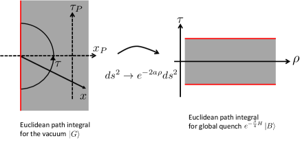
Next, we consider the Rindler quenches. In this problem, we start from the ground state of the homogeneous Hamiltonian on a half line . Then, we change the Hamiltonian to the Rindler Hamiltonian and evolve the original state by the Rindler Hamiltonian. Here is a parameter of the dimension of the inverse of the length. This is equivalent to putting CFT on a curved spacetime
| (II.3) |
Then, the evolution of entanglement entropy for an infinite line is given by
| (II.4) |
Two quench problems show a similar evolution of entanglement entropy. Actually, after identifying the parameter and changing the cutoff , the entropy for a global quench becomes
| (II.5) |
and we can obtain exactly the same evolution of the entropy for Rindler quenches.
Actually, these two problems are related in a more direct manner. First, the Euclidean version of the metric (II.3) is
| (II.6) |
where we used the coordinate transformation
| (II.7) |
The coordinate transformation suggests that the ground state of the homogeneous Hamiltonian is equivalent to the boundary state with the finite amount of Euclidean evolution by the Rindler Hamiltonian:
| (II.8) |
Next, changing the spacial coordinate , we obtain
| (II.9) |
which means that after Weyl transformation , the Euclidean path integral is equivalent to that of Calabrese-Cardy state preparation for global quenches [39, 40, 32]. These two show that the correlation functions after Rindler quench is Weyl equivalent to those after global quenches:
| (II.10) |
In particular, we can apply this relation to twist operators to study entanglement entropy and we can deduce the relation (II.5). In this manner, we can explain the relation between Rindler quench and global quench following their path integral representations and coordinate transformations among them.
III Local quench on finite strips
In Ref. [28], the authors studied a local quantum quench process in the context of (1+1)d CFT. In this process, the system is initially “cut” into two independent subsystems. To be specific, we consider two intervals of equal length (, , and . (Here, denoting the total system size by may look bizarre. The motivation for this will become clear when we later make contact with the Möbius quench.) The system is initially prepared as the tensor product of the ground states of the two intervals. These two intervals are then glued together at time . Namely, for , the system time-evolves by the Hamiltonian for the single interval of length .
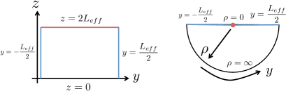
The quench process can be analyzed by using the Euclidean path integral on a “pants” geometry, which is represented in Fig. 2. We use to coordinatize this geometry where and represent Euclidean temporal and spatial coordinates, respectively. We regularize this excited state by the Euclidean path integral for Euclidean time .
The Euclidean geometry is mapped to the upper half plane by the conformal transformation [28]
| (III.1) |
Physical observables can then be computed from the corresponding correlations on the upper half-plane. For example, the one -oint function of a primary operator with conformal dimension where is a primary operator, is the scaling dimension of with the conformal weight and is the one point function. Introducing the mapping to the strip , which will use later, we can also write the map as
| (III.2) |
The entanglement entropy can be obtained from the correlation function of the twist-anti-twist operators [41]. The Euclidean time is analytically continued to Lorentzian time , . For general , and for the subsystem of an interval , we obtain the following expression for the entanglement entropy:
| (III.3) |
where is the central charge, is a UV cutoff, and
| (III.4) |
In particular, at , the entanglement entropy just after joining is
| (III.5) |
Here is a UV cutoff. The profile of the dynamical entanglement entropy is plotted in Fig. 3. Here, we consider the difference between (III.3) and the ground state entanglement entropy, where is the entanglement entropy of the ground state on the same strip.
The conformal map (III.1) to the upper half-plane also allows us to compute the time-dependence of the energy-momentum tensor by
| (III.6) |
Explicitly, the holomorphic and anti-holomorphic components of the energy-momentum tensor are given by
| (III.7) |
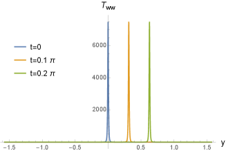
In Fig. 4, we plot the right-moving part of the stress tensor. Right at the moment of the quench, the stress tensor is sharply peaked at , and then propagates to the right. Once the peaks hit the boundaries at , they get reflected back. After that the energy-momentum tensor profile exhibits an eternal oscillation. Note that at the peak looks like to jump from one boundary to the other. This jump actually captures the reflection correctly since the right moving excitation is reflected to the left moving excitation at the boundaries.
IV Möbius quench
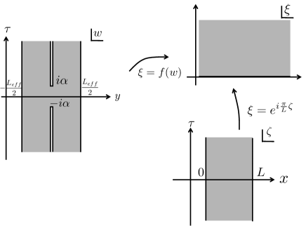
In this section, we consider another quantum quench problem, the Möbius quench [9], which is seemingly different from the local quantum quench considered in the previous section. In the Möbius quench, we start from the ground state of (1+1)d CFT on a finite interval of length , . Here, is the (regular) Hamiltonian of CFT on a finite interval, and given in terms of the energy density operator as . At , we suddenly change the Hamiltonian from to the Möbius Hamiltonian with
| (IV.1) |
Here, is a real positive parameter. As we send and , the Möbius Hamiltonian reduces to the regular Hamiltonian and the sine-square deformed (SSD) Hamiltonian, respectively [5, 44, 6, 45, 46, 47, 7, 48, 49, 8, 50, 51, 52, 53, 11, 54, 55, 56, 57, 58, 59]. In [10], the Möbius quench starting from a thermal initial state was studied. In holographic theories, the Möbius quench induces a non-trivial dynamics (time-dependent deformation) of the black hole horizon. As we will demonstrate later, the current Möbius quench induces a non-trivial dynamics of the EOW brane.
The Möbius Hamiltonian effectively changes the total system size from to where and are related by [52, 53]
| (IV.2) |
Specifically, there is a conformal transformation that maps the spacetime (cylinder of circumference ) with as the Hamiltonian, to another spacetime (cylinder of circumference ) with as the Hamiltonian. In the limit (the SSD limit), .
IV.1 The equivalence between the Möbius quench and the local quench on finite strips
We now establish the equivalence between the local quantum quench in the previous section and the Möbius quench. To this end, we first study the relationship between the flat metric and the Möbius Hamiltonian. The time-evolution generated by the Möbius Hamiltonian is spatially inhomogeneous and corresponds to the metric
| (IV.3) |
The relation between flat metric and the Möbius Hamiltonian can be read off from
| (IV.4) |
where the Weyl factor is given by
| (IV.5) |
and and are related by the coordinate transformation
| (IV.6) |
By taking while keeping , we can take the SSD limit. The coordinate transformation in the SSD limit is then given by
| (IV.7) |
Here, runs from to whereas runs from to . The latter relation is written as
| (IV.8) |
The coordinate transformation (IV.6) allows us to relate the flat metric and inhomogeneous metric corresponding to the Möbius Hamiltonian. In particular, the ground state entanglement entropy of the two problems are related. Since the Möbius Hamiltonian shares the same ground state as the regular Hamiltonian , the entanglement entropy of the ground state (on a finite interval of length ) is given by
| (IV.9) |
where the subsystem is the interval . By the coordinate change (IV.6) and the Weyl transformation of the cutoff,
| (IV.10) |
the entanglement entropy (IV.9) becomes
| (IV.11) |
Here, satisfies
| (IV.12) |
or more explicitly is given as a function of by
| (IV.13) |
This equation establishes the relation between the parameter in local quenches, which characterizes the energy scale (and the localization length of the excitation) of the initial state, and the that characterizes the inhomogeneity of the Möbius deformation. In particular, Möbius quench with an inhomogeneity parameter is related to a local quench with the specific parameter which is determined by (IV.13). The same strategy can be used to establish the relationship between these two problems for . Once again, by coordinate change and the Weyl transformation the entanglement entropy for the local quench (III.3) on a finite strip becomes
| (IV.14) |
Here
| (IV.15) |
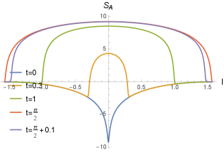
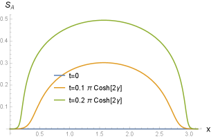
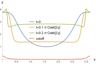
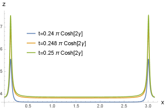
This is exactly the time evolution of entanglement entropy after the Möbius quench found in [9]. This suggests that the Möbius quench is obtained from the local quench on the coordinate through the Weyl (IV.5) and coordinate (IV.4) transformations. The evolution of entanglement entropy is shown in Fig. 5, where we consider dynamical entanglement entropy with subtraction of the entanglement entropy .
Comparing (III.2) and (IV.6), if we identify , the conformal map for the local quench (III.2) gives the holomorphic extension of the spatial coordinate transformation (IV.6) for the Möbius quench. This corresponds to finding the Euclidean path integral representation of the homogeneous ground state using the Möbius Hamiltonian. This is somewhat similar to the ground state of on an infinite line that can also be interpreted as the thermofield double state for the Rindler Hamiltonian.
The conformal symmetry implies that when we consider the sudden quench to the Möbius Hamiltonian with the envelop function , there is no time evolution. This can be thought of as a BCFT counterpart of the coincidence of the ground states of the Möbius and the homogeneous Hamiltonians. On the other hand, in the Möbius quench we shorten the period of the envelop function , which leads to the branch cut structure in (IV.6) and leads to the excitation for the Möbius Hamiltonian. Because of the symmetry of the envelop function and the homogeneous ground state, it is natural to expect that the excitation concentrates near the center . What we find is that such a local excitation is represented by the Euclidean path integral (III.2) for local quenches where the sharp excitation is located near the center but smeared by the regularization .
Mapping the Möbius quench to the local quench makes it easy to calculate the stress tensor profile. The stress tensor of the Weyl transformed metric is given by
| (IV.16) |
where is the stress tensor in the flat metric and is
| (IV.17) |
In the coordinate becomes
| (IV.18) |
On the other hand, becomes
| (IV.19) |
where and are given by
| (IV.20) | ||||
| (IV.21) |
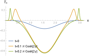
where we defined a function . At , the full stress tensor (IV.16) has relatively simple expression as
| (IV.22) |
V Holographic dual descriptions of quenches
V.1 Holographic dual of local quenches on finite strips
The equivalence we have established allows us to construct the holographic dual description of one of these quenches starting from that of the other. Here, we first discuss the holographic dual description of the local quantum quench. We will later use it to derive the holographic dual of the Möbius quench. As the relevant Euclidean path integral is defined on the upper half-plane, the bulk description is given in terms of AdS/BCFT [37, 38, 60]. In AdS/BCFT, what corresponds to BCFT is the bulk AdS space with an end-of-the-world (EOW) brane.
Adopting to our setup, we expect that the EOW is non-stationary in time. For the time evolution of states with Euclidean path integral preparation, we can consider the EOW profile in the following manner [61]. We start from CFT defined on the upper half-plane. The relevant bulk geometry is AdS with the EOW brane with the metric in given by
| (V.1) |
Assuming the case of tensionless EOW brane for simplicity, the EOW brane location in is simply given by .
We now consider the conformal transformation (III.1) that connects the upper half-plane and the pants geometry. In Euclidean signature, the conformal transformation at the boundary
| (V.2) |
is extended to the bulk as [62]
| (V.3) |
After the coordinate transformation, the metric in coordinate is
| (V.4) |
which is the general solution of the three-dimensional Einstein gravity [63]. Here
| (V.5) |
In coordinate, the EOW brane location is given by . Rewriting this condition as , we obtain
| (V.6) |
We can apply the above general prescription for the stress tensor and the EOW profile to the conformal map (III.1). We already studied the energy-momentum tensor in (III.7). On the other hand, the EOW brane profile is given by
| (V.7) |
where the numerator and the denominator are given by
| (V.8) | ||||
| (V.9) |
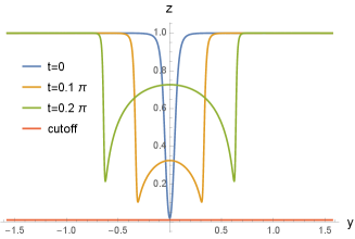
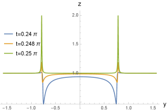
The EOW brane profile calculated from (V.7) is shown in Fig. 7. Right at the moment of the quench, the EOW is sharply peaked at , and almost “touches” the boundary. For , the peak splits into left- and right-moving ones. They propagate away from the . These behaviors are consistent with the time-dependence of the stress-energy tensor. For later times, the EOW profile looks more complicated.
We note that in the original Poincare coordinate (V.1), the EOW intersects with the asymptotic boundary. This does not appear to be the case in Fig. 7. As is the physical boundaries, we may expect that the EOW intersects with the asymptotic boundary at these points. The reason for this may be that our coordinates are “not good.” It is useful to illustrate what happens in the example of pure global AdS3. This corresponds to the limit where we do not have any excitation. The relevant conformal transformation is obtained by the limit of (III.1), which leads to
| (V.10) |
The stress tensor (III) becomes . From this, the metric (V.4) becomes
| (V.11) |
This is actually the global AdS3 metric. Changing the coordinate makes it easy to see the equivalence to the global AdS3. In this coordinate system, the metric is
| (V.12) |
On the other hand, using the map (V.10) in (V.6) the brane profile becomes
| (V.13) |
This actually corresponds to , which is just a point in a constant slice. On the other hand, in the global AdS3 case, the tensionless EOW profile is known to be given by the solution of [64]
| (V.14) |
Therefore, the EOW brane is located at and also at , as depicted in Fig. 8. However, we are missing the part in the formula (V.6).
What we expect for the local quench is essentially the same. The counterpart of is captured by (V.7) though they are generically a codimension one object rather than a point in plane, which is codimension two. We expect that we are missing the counterpart of in the brane motion in the local quench problem. We note that this missing problem does not occur in the local quench on an infinite line [61] where the EOW brane intersects with the AdS boundary at infinity. It is interesting to comprehensively understand when this problem occurs and how to remedy it, but we leave it to a future problem.
Note that the dynamics of the EOW brane in Fig. 7 looks similar to the entanglement dynamics in Fig. 3. Through the holographic entanglement entropy formula [65, 66, 67], the entanglement entropy measures the distance between AdS boundary and the EOW brane. The qualitative resemblance reflects this connection between spacetime geometry and entanglement.
V.2 Holographic dual of Möbius quench
Now we can construct the holographic dual of the Möbius quench since we know the map from Möbius quench to the local quench on a finite strip, and also the holographic dual of the latter. The dual geometry is given by
| (V.15) |
where the stress tensor profile is given by (IV.19). Now the cutoff is given by (IV.10), which is position dependent. This position-dependent cutoff reproduces the part of stress tensor (IV.18) that comes from the Weyl transformation. Because the dual geometry is given by the dual geometry of the local quench with in (IV.12), we can use the EOW profile (V.7). By changing the coordinate from to using the diffeomorphism (IV.12), we obtain the EOW profile for the dual of Möbius quenches. The result is given by
| (V.16) |
where the numerator and the denominator are given by
| (V.17) | |||
| (V.18) |
Here we recall and . After analytically continuing to the Lorentzian time , we obtain the time dependence of the EOW profile.
VI Conclusion
In this paper, we studied the dynamics after the local quench on finite intervals and the Möbius quench in (1+1)d CFT. First, we found that the Möbius quench can be obtained from the local quench by diffeomorphism and Weyl transformations. In the holographic setups, we employ the AdS/BCFT correspondence and study the motion of the EOW brane. We also compare this brane motion with the entanglement dynamics for an interval. The brane dynamics qualitatively agrees with the entanglement dynamics.
There is in principle a vast class of quantum quench problems that we can consider in (1+1)d CFT. As demonstrated here, we expect that some of them are related to each other. It would be interesting to explore this type of equivalence relation further beyond the specific examples considered in this paper. This may lead to a classification of possible dynamical behaviors using the equivalence relation.
Acknowledgements.
SR is supported by the National Science Foundation under Award No. DMR-2001181, and by a Simons Investigator Grant from the Simons Foundation (Award No. 566116). TN is supported by MEXT KAKENHI Grant-in-Aid for Transformative Research Areas A “Extreme Universe” (22H05248) and JSPS KAKENHI Grant-in-Aid for Early-Career Scientists (23K13094). MN is supported by funds from University of Chinese Academy of Sciences (UCAS), and funds from the Kavli Institute for Theoretical Sciences (KITS). MT is supported by an appointment to the YST Program at the APCTP through the Science and Technology Promotion Fund and Lottery Fund of the Korean Government. MT is also supported by the Korean Local Governments - Gyeongsangbuk-do Province and Pohang City. JKF is supported by the Institute for Advanced Study and the National Science Foundation under Grant No. PHY-2207584. This work is supported by the Gordon and Betty Moore Foundation through Grant GBMF8685 toward the Princeton theory program.References
- [1] P. W. Anderson, “Absence of diffusion in certain random lattices,” Phys. Rev. 109 (Mar, 1958) 1492–1505.
- [2] I. Bloch, J. Dalibard, and W. Zwerger, “Many-body physics with ultracold gases,” Reviews of Modern Physics 80 no. 3, (July, 2008) 885–964, arXiv:0704.3011 [cond-mat.other].
- [3] J. Dubail, J.-M. Stéphan, J. Viti, and P. Calabrese, “Conformal Field Theory for Inhomogeneous One-dimensional Quantum Systems: the Example of Non-Interacting Fermi Gases,” SciPost Phys. 2 (2017) 002. https://scipost.org/10.21468/SciPostPhys.2.1.002.
- [4] N. D. Birrell and P. C. W. Davies, Quantum Fields in Curved Space. Cambridge Monographs on Mathematical Physics. Cambridge Univ. Press, Cambridge, UK, 2, 1984.
- [5] A. Gendiar, R. Krcmar, and T. Nishino, “Spherical Deformation for One-Dimensional Quantum Systems,” Progress of Theoretical Physics 122 no. 4, (Oct., 2009) 953–967, arXiv:0810.0622 [cond-mat.str-el].
- [6] T. Hikihara and T. Nishino, “Connecting distant ends of one-dimensional critical systems by a sine-square deformation,” Phys. Rev. B 83 no. 6, (Feb., 2011) 060414, arXiv:1012.0472 [cond-mat.stat-mech].
- [7] H. Katsura, “Sine-square deformation of solvable spin chains and conformal field theories,” Journal of Physics A Mathematical General 45 no. 11, (Mar., 2012) 115003, arXiv:1110.2459 [cond-mat.stat-mech].
- [8] T. Tada, “Sine-square deformation and its relevance to string theory,” Modern Physics Letters A 30 (May, 2015) 1550092, arXiv:1404.6343 [hep-th].
- [9] X. Wen and J.-Q. Wu, “Quantum dynamics in sine-square deformed conformal field theory: Quench from uniform to nonuniform conformal field theory,” Phys. Rev. B 97 no. 18, (May, 2018) 184309, arXiv:1802.07765 [cond-mat.str-el].
- [10] K. Goto, M. Nozaki, K. Tamaoka, M. Tian Tan, and S. Ryu, “Non-Equilibrating a Black Hole with Inhomogeneous Quantum Quench,” arXiv e-prints (Dec., 2021) arXiv:2112.14388, arXiv:2112.14388 [hep-th].
- [11] X. Wen and J.-Q. Wu, “Floquet conformal field theory,” arXiv e-prints (Apr., 2018) arXiv:1805.00031, arXiv:1805.00031 [cond-mat.str-el].
- [12] B. Lapierre and P. Moosavi, “Geometric approach to inhomogeneous Floquet systems,” Phys. Rev. B 103 no. 22, (June, 2021) 224303, arXiv:2010.11268 [cond-mat.stat-mech].
- [13] N. Allegra, J. Dubail, J.-M. Stéphan, and J. Viti, “Inhomogeneous field theory inside the arctic circle,” Journal of Statistical Mechanics: Theory and Experiment 5 no. 5, (May, 2016) 053108, arXiv:1512.02872 [cond-mat.stat-mech].
- [14] J. Dubail, J.-M. Stéphan, and P. Calabrese, “Emergence of curved light-cones in a class of inhomogeneous Luttinger liquids,” SciPost Physics 3 no. 3, (Sept., 2017) 019, arXiv:1705.00679 [cond-mat.str-el].
- [15] K. Gawedzki, E. Langmann, and P. Moosavi, “Finite-Time Universality in Nonequilibrium CFT,” Journal of Statistical Physics 172 no. 2, (July, 2018) 353–378, arXiv:1712.00141 [cond-mat.stat-mech].
- [16] E. Langmann and P. Moosavi, “Diffusive Heat Waves in Random Conformal Field Theory,” Phys. Rev. Lett. 122 no. 2, (Jan., 2019) 020201, arXiv:1807.10239 [cond-mat.stat-mech].
- [17] I. MacCormack, A. Liu, M. Nozaki, and S. Ryu, “Holographic duals of inhomogeneous systems: the rainbow chain and the sine-square deformation model,” Journal of Physics A Mathematical General 52 no. 50, (Dec., 2019) 505401, arXiv:1812.10023 [cond-mat.str-el].
- [18] J. J. Bisognano and E. H. Wichmann, “On the Duality Condition for a Hermitian Scalar Field,” J. Math. Phys. 16 (1975) 985–1007.
- [19] J. J. Bisognano and E. H. Wichmann, “On the Duality Condition for Quantum Fields,” J. Math. Phys. 17 (1976) 303–321.
- [20] J. M. Maldacena, “The Large N limit of superconformal field theories and supergravity,” Int. J. Theor. Phys. 38 (1999) 1113–1133, arXiv:hep-th/9711200 [hep-th]. [Adv. Theor. Math. Phys.2,231(1998)].
- [21] D. L. Jafferis, A. Lewkowycz, J. Maldacena, and S. J. Suh, “Relative entropy equals bulk relative entropy,” JHEP 06 (2016) 004, arXiv:1512.06431 [hep-th].
- [22] B. Czech, J. L. Karczmarek, F. Nogueira, and M. Van Raamsdonk, “The Gravity Dual of a Density Matrix,” Class. Quant. Grav. 29 (2012) 155009, arXiv:1204.1330 [hep-th].
- [23] X. Dong, D. Harlow, and A. C. Wall, “Reconstruction of Bulk Operators within the Entanglement Wedge in Gauge-Gravity Duality,” Phys. Rev. Lett. 117 no. 2, (2016) 021601, arXiv:1601.05416 [hep-th].
- [24] T. Faulkner and A. Lewkowycz, “Bulk locality from modular flow,” JHEP 07 (2017) 151, arXiv:1704.05464 [hep-th].
- [25] T. Faulkner, M. Li, and H. Wang, “A modular toolkit for bulk reconstruction,” JHEP 04 (2019) 119, arXiv:1806.10560 [hep-th].
- [26] Y. Chen, X. Dong, A. Lewkowycz, and X.-L. Qi, “Modular Flow as a Disentangler,” JHEP 12 (2018) 083, arXiv:1806.09622 [hep-th].
- [27] Xinyu Liu, Alexander McDonald, Tokiro Numasawa, Biao Lian, Shinsei Ryu, to be published.
- [28] J.-M. Stéphan and J. Dubail, “Local quantum quenches in critical one-dimensional systems: entanglement, the Loschmidt echo, and light-cone effects,” Journal of Statistical Mechanics: Theory and Experiment 2011 no. 8, (Aug., 2011) 08019, arXiv:1105.4846 [cond-mat.stat-mech].
- [29] P. Calabrese and J. Cardy, “Time Dependence of Correlation Functions Following a Quantum Quench,” Phys. Rev. Lett. 96 no. 13, (Apr., 2006) 136801, arXiv:cond-mat/0601225 [cond-mat.stat-mech].
- [30] P. Calabrese and J. Cardy, “Quantum quenches in extended systems,” Journal of Statistical Mechanics: Theory and Experiment 2007 no. 6, (June, 2007) 06008, arXiv:0704.1880 [cond-mat.stat-mech].
- [31] P. Calabrese and J. Cardy, “Entanglement and correlation functions following a local quench: a conformal field theory approach,” Journal of Statistical Mechanics: Theory and Experiment 2007 no. 10, (Oct., 2007) 10004, arXiv:0708.3750 [cond-mat.stat-mech].
- [32] P. Calabrese and J. Cardy, “Quantum quenches in 1 + 1 dimensional conformal field theories,” Journal of Statistical Mechanics: Theory and Experiment 6 no. 6, (June, 2016) 064003, arXiv:1603.02889 [cond-mat.stat-mech].
- [33] D. Bernard and B. Doyon, “Energy flow in non-equilibrium conformal field theory,” Journal of Physics A Mathematical General 45 no. 36, (Sept., 2012) 362001, arXiv:1202.0239 [cond-mat.str-el].
- [34] D. Bernard and B. Doyon, “Non-Equilibrium Steady States in Conformal Field Theory,” Annales Henri Poincaré 16 no. 1, (Jan., 2015) 113–161, arXiv:1302.3125 [math-ph].
- [35] D. Bernard and B. Doyon, “Conformal field theory out of equilibrium: a review,” Journal of Statistical Mechanics: Theory and Experiment 6 no. 6, (June, 2016) 064005, arXiv:1603.07765 [cond-mat.stat-mech].
- [36] X. Wen, “Bridging global and local quantum quenches in conformal field theories,” arXiv:1611.00023 [cond-mat.str-el].
- [37] T. Takayanagi, “Holographic Dual of BCFT,” Phys. Rev. Lett. 107 (2011) 101602, arXiv:1105.5165 [hep-th].
- [38] M. Fujita, T. Takayanagi, and E. Tonni, “Aspects of AdS/BCFT,” JHEP 11 (2011) 043, arXiv:1108.5152 [hep-th].
- [39] P. Calabrese and J. Cardy, “Evolution of entanglement entropy in one-dimensional systems,” Journal of Statistical Mechanics: Theory and Experiment 2005 no. 4, (Apr., 2005) 04010, arXiv:cond-mat/0503393 [cond-mat.stat-mech].
- [40] T. Hartman and J. Maldacena, “Time evolution of entanglement entropy from black hole interiors,” Journal of High Energy Physics 2013 (May, 2013) 14, arXiv:1303.1080 [hep-th].
- [41] P. Calabrese and J. Cardy, “Entanglement entropy and quantum field theory,” Journal of Statistical Mechanics: Theory and Experiment 2004 no. 6, (June, 2004) 06002, arXiv:hep-th/0405152 [hep-th].
- [42] K. Kuns and D. Marolf, “Non-Thermal Behavior in Conformal Boundary States,” JHEP 09 (2014) 082, arXiv:1406.4926 [cond-mat.stat-mech].
- [43] G. Mandal, R. Sinha, and T. Ugajin, “Finite size effect on dynamical entanglement entropy: CFT and holography,” arXiv:1604.07830 [hep-th].
- [44] A. Gendiar, M. Daniška, Y. Lee, and T. Nishino, “Suppression of finite-size effects in one-dimensional correlated systems,” Phys. Rev. A 83 no. 5, (May, 2011) 052118, arXiv:1012.1472 [cond-mat.str-el].
- [45] N. Shibata and C. Hotta, “Boundary effects in the density-matrix renormalization group calculation,” Phys. Rev. B 84 no. 11, (Sept., 2011) 115116, arXiv:1106.6202 [cond-mat.str-el].
- [46] I. Maruyama, H. Katsura, and T. Hikihara, “Sine-square deformation of free fermion systems in one and higher dimensions,” Phys. Rev. B 84 no. 16, (Oct., 2011) 165132, arXiv:1108.2973 [cond-mat.stat-mech].
- [47] H. Katsura, “Exact ground state of the sine-square deformed XY spin chain,” Journal of Physics A Mathematical General 44 no. 25, (June, 2011) 252001, arXiv:1104.1721 [cond-mat.stat-mech].
- [48] C. Hotta and N. Shibata, “Grand canonical finite-size numerical approaches: A route to measuring bulk properties in an applied field,” Phys. Rev. B 86 no. 4, (July, 2012) 041108, arXiv:1307.3713 [cond-mat.str-el].
- [49] C. Hotta, S. Nishimoto, and N. Shibata, “Grand canonical finite size numerical approaches in one and two dimensions: Real space energy renormalization and edge state generation,” Phys. Rev. B 87 (Mar, 2013) 115128.
- [50] N. Ishibashi and T. Tada, “Infinite circumference limit of conformal field theory,” Journal of Physics A Mathematical General 48 no. 31, (Aug., 2015) 315402, arXiv:1504.00138 [hep-th].
- [51] N. Ishibashi and T. Tada, “Dipolar quantization and the infinite circumference limit of two-dimensional conformal field theories,” International Journal of Modern Physics A 31 no. 32, (Nov., 2016) 1650170, arXiv:1602.01190 [hep-th].
- [52] K. Okunishi, “Sine-square deformation and Möbius quantization of 2D conformal field theory,” PTEP 2016 no. 6, (2016) 063A02, arXiv:1603.09543 [hep-th].
- [53] X. Wen, S. Ryu, and A. W. W. Ludwig, “Evolution operators in conformal field theories and conformal mappings: Entanglement Hamiltonian, the sine-square deformation, and others,” Phys. Rev. B 93 no. 23, (June, 2016) 235119, arXiv:1604.01085 [cond-mat.str-el].
- [54] R. Fan, Y. Gu, A. Vishwanath, and X. Wen, “Emergent Spatial Structure and Entanglement Localization in Floquet Conformal Field Theory,” Physical Review X 10 no. 3, (July, 2020) 031036, arXiv:1908.05289 [cond-mat.str-el].
- [55] B. Han and X. Wen, “Classification of SL2 deformed Floquet conformal field theories,” Phys. Rev. B 102 no. 20, (Nov., 2020) 205125, arXiv:2008.01123 [cond-mat.stat-mech].
- [56] R. Fan, Y. Gu, A. Vishwanath, and X. Wen, “Floquet conformal field theories with generally deformed Hamiltonians,” SciPost Phys. 10 no. 2, (2021) 049, arXiv:2011.09491 [hep-th].
- [57] X. Wen, R. Fan, A. Vishwanath, and Y. Gu, “Periodically, quasiperiodically, and randomly driven conformal field theories,” Physical Review Research 3 no. 2, (Apr., 2021) 023044, arXiv:2006.10072 [cond-mat.stat-mech].
- [58] B. Lapierre, K. Choo, C. Tauber, A. Tiwari, T. Neupert, and R. Chitra, “Emergent black hole dynamics in critical Floquet systems,” Physical Review Research 2 no. 2, (Apr., 2020) 023085, arXiv:1909.08618 [cond-mat.str-el].
- [59] B. Lapierre, K. Choo, A. Tiwari, C. Tauber, T. Neupert, and R. Chitra, “Fine structure of heating in a quasiperiodically driven critical quantum system,” Physical Review Research 2 no. 3, (Sep, 2020) . http://dx.doi.org/10.1103/PhysRevResearch.2.033461.
- [60] M. Nozaki, T. Takayanagi, and T. Ugajin, “Central charges for BCFTs and holography,” Journal of High Energy Physics 2012 (June, 2012) 66, arXiv:1205.1573 [hep-th].
- [61] P. Caputa, T. Numasawa, T. Shimaji, T. Takayanagi, and Z. Wei, “Double Local Quenches in 2D CFTs and Gravitational Force,” JHEP 09 (2019) 018, arXiv:1905.08265 [hep-th].
- [62] M. M. Roberts, “Time evolution of entanglement entropy from a pulse,” JHEP 12 (2012) 027, arXiv:1204.1982 [hep-th].
- [63] M. Banados, “Three-dimensional quantum geometry and black holes,” AIP Conf. Proc. 484 no. 1, (1999) 147–169, arXiv:hep-th/9901148.
- [64] T. Numasawa, “Holographic Complexity for disentangled states,” PTEP 2020 no. 3, (2020) 033B02, arXiv:1811.03597 [hep-th].
- [65] S. Ryu and T. Takayanagi, “Holographic derivation of entanglement entropy from AdS/CFT,” Phys. Rev. Lett. 96 (2006) 181602, arXiv:hep-th/0603001.
- [66] S. Ryu and T. Takayanagi, “Aspects of Holographic Entanglement Entropy,” JHEP 08 (2006) 045, arXiv:hep-th/0605073.
- [67] V. E. Hubeny, M. Rangamani, and T. Takayanagi, “A Covariant holographic entanglement entropy proposal,” JHEP 07 (2007) 062, arXiv:0705.0016 [hep-th].