Brownian snails with removal:
epidemics in diffusing populations
Abstract.
Two stochastic models of susceptible/infected/removed (SIR) type are introduced for the spread of infection through a spatially-distributed population. Individuals are initially distributed at random in space, and they move continuously according to independent diffusion processes. The disease may pass from an infected individual to an uninfected individual when they are sufficiently close. Infected individuals are permanently removed at some given rate . Such processes are reminiscent of so-called frog models, but differ through the action of removal, as well as the fact that frogs jump whereas snails slither.
Two models are studied here, termed the ‘delayed diffusion’ and the ‘diffusion’ models. In the first, individuals are stationary until they are infected, at which time they begin to move; in the second, all individuals start to move at the initial time . Using a perturbative argument, conditions are established under which the disease infects a.s. only finitely many individuals. It is proved for the delayed diffusion model that there exists a critical value for the survival of the epidemic.
Key words and phrases:
Percolation, infectious disease, SIR model, frog model, snail model, epidemic, diffusion, Wiener sausage2010 Mathematics Subject Classification:
60K35, 60G151. Introduction
1.1. Outline of the models
Numerous mathematical models have been introduced to describe the spread of a disease around a population. Such models may be deterministic or stochastic, or a mixture of each; they may incorporate a range of factors including susceptibility, infectivity, recovery, and removal; the population members (termed ‘particles’) may be distributed about some given space; and so on. We propose two models in which (i) the particles move randomly about the space that they inhabit, (ii) infection may be passed between particles that are sufficiently close to one another, and (iii) after the elapse of a random time since infection, a particle is removed from the process. These models differ from that of Beckman, Dinan, Durrett, Huo, and Junge [3] through the introduction of the permanent ‘removal’ of particles, and this new feature brings a significant new difficulty to the analysis.
We shall concentrate mostly on the case in which the particles inhabit where . Here is a concrete example of the processes studied here.
-
(a)
Particles are initially distributed in in the manner of a rate- Poisson process conditioned to contain a point at the origin .
-
(b)
Particles move randomly within according to independent Brownian motions with variance-parameter .
-
(c)
At time the particle at the origin (the initial ‘infective’) suffers from an infectious disease, which may be passed to others when sufficiently close.
-
(d)
When two particles, labelled and , are within a given distance , and is already infected, then particle becomes infected.
-
(e)
Each particle is infected for a total period of time having the exponential distribution with parameter , and is then permanently removed.
The fundamental question is to determine for which vectors it is the case that (with strictly positive probability) infinitely many particles become infected. For simplicity, we shall assume henceforth that
| (1.1) |
We shall generally assume . In the special case , (studied in [3]) a particle once infected remains infected forever, and the subsequent analysis is greatly facilitated by a property of monotonicity that is absent in the more challenging case considered in the current work.
Two protocols for movement feature in this article.
-
A.
Delayed diffusion model. The initial infective starts to move at time , and all other particles remain stationary until they are infected, at which times they begin to move.
-
B.
Diffusion model. All particles begin to move at time .
The main difficulty in studying these models arises from the fact that particles are permanently removed after a (random) period of infectivity. This introduces a potential non-monotonicity into the model, namely that the presence of infected particles may hinder the growth of the process through the creation of islands of ‘removed’ particles that can act as barriers to the further spread of infection. A related situation (but without the movement of particles) was considered by Kuulasma [21] in a discrete setting, and the methods derived there are useful in our Section 3.7 (see also Alves et al. [1, p. 4]). This issue may be overcome for the delayed diffusion model, but remains problematic in the case of the diffusion process.
Let denote the set of particles that are ever infected, and
| (1.2) |
We say the process
| becomes extinct | |||
| survives |
Let denote the critical value of for the disk (or ‘Boolean’) percolation model with radius on (see, for example, [25]). It is immediate for both models above that
| (1.3) |
since in that case the disease spreads instantaneously to the percolation cluster containing the initial infective, and in addition we have .
1.2. Two exemplars of results
We write (respectively, ) for the function of (1.2) in the case of the diffusion model (respectively, delayed diffusion model). The following two theorems are proved in Sections 3 and 4 as special cases of results for more general epidemic models than those given above.
Theorem 1.1 (Brownian delayed diffusion model).
Let . There exists a non-decreasing function such that
| (1.4) |
Furthermore, when , and there exists such that when .
Theorem 1.2 (Brownian diffusion model).
Let . There exists and a non-decreasing function such that when and .
For the diffusion model, we have no proof of survival for and small positive (that is, that for some and ), and neither does the current work answer the question of whether or not survival ever occurs when . See Section 4.3. The above theorems are proved using a perturbative argument, and thus fall short of the assertion that .
The methods of proof may be made quantitative, leading to bounds for the numerical values of the critical points . Such bounds are far from precise, and therefore we do not explore them here. Our basic estimates for the growth of infection hold if the intensity of the Poisson process is non-constant so long as it is bounded uniformly between two strictly positive constants. The existence of the subcritical phase may be proved for more general diffusions than Brownian motion.
1.3. Literature and notation
The related literature is somewhat ramified, and a spread of related problems have been studied by various teams. We mention a selection of papers but do not attempt a full review, and we concentrate on works associated with rather than with trees or complete graphs.
The delayed diffusion model may be viewed as a continuous-time version of the ‘frog’ random walk process studied in Alves et al. [1, 2], Ramirez and Sidoravicius [29], Fontes et al. [7], Benjamini et al. [4], and Hoffman, Johnson, and Junge [15, 16]. See Popov [28] for an early review. Kesten and Sidoravicius [17, 18, 19] considered a variant of the frog model as a model for infection, both with and without recuperation (that is, when infected frogs recover and become available for reinfection—see also Section 4.3 of the current work). The paper of Beckman et al. [3] is devoted to the delayed diffusion model without removal (that is, with ). Peres et al. [27] studied three geometric properties of a Poissonian/Brownian cloud of particles, in work inspired in part by the dynamic Boolean percolation model of van den Berg et al. [5]. Related work has appeared in Gracar and Stauffer [9].
A number of authors have considered the frog model with recuperation under the title ‘activated random walks’. The reader is referred to the review by Rolla [30], and for recent work to Stauffer and Taggi [33] and Rolla et al. [31].
We write and (or ) for the indicator function of an event or set . Let denote the closed -ball of with centre at the origin, and . The -dimensional Lebesgue measure of a set is written , and the Euclidean norm . The radius of is defined by
We abbreviate (respectively, ) to the generic notation (respectively, ).
The contents of this paper are as follows. The two models are defined in Section 2 with a degree of generality that includes general diffusions and a more general process of infection. The delayed diffusion model is studied in Section 3, and the diffusion model in Section 4. Theorem 1.1 (respectively, Theorem 1.2) is contained within Theorem 3.1 (respectively, Theorem 4.1).
1.4. Open problems
This introduction closes with a short account of some of the principal remaining open problems. For concreteness, we restrict ourselves to the Brownian models of Section 1.2 without further reference to the random-walk versions of these models, and the general models of Section 2.1. This section is positioned here despite the fact that it refers sometimes to versions of the models that have not yet been fully introduced (see Section 2).
-
A.
For the Brownian delayed diffusion model, show that the critical value of Theorem 1.1 satisfies whenever .
-
B.
When , prove survival in the Brownian diffusion model for some and small . More specifically, show that for suitable and .
-
C.
Having resolved problem B, show the existence of a critical value for the Brownian diffusion model such that survival occurs when and not when . Furthermore, identify the set of such that .
-
D.
Decide whether or not survival can ever occur for the Brownian diffusion model in one dimension.
-
E.
In either model, prove a shape theorem for the set of particles that are either infected or removed at time .
2. General models
2.1. The general set-up
Let . A diffusion process in is a solution to the stochastic differential equation
| (2.1) |
where is a standard Brownian motion in . (We may write either or .) For definiteness, we shall assume that: ; has continuous sample paths; the instantaneous drift vector and variance matrix are locally Lipschitz continuous. We do not allow , to be time-dependent. We call the process ‘Brownian’ if is a standard Brownian motion, which is to say that is the zero vector and is the identity matrix.
Let be such a diffusion, and let be independent copies of . Let , , and let be integrable with
| (2.2) |
We call radially decreasing if
| (2.3) |
Let be a Poisson process on (conditioned to possess a point at the origin ) with constant intensity . At time , particles with label-set are placed at the respective points . We may refer to a particle by either its index or its initial position .
We describe the process of infection in a somewhat informal manner (see also Section 2.4). For , at any given time particle is in one of three states S (susceptible), I (infected), and R (removed). Thus the state space is , and we write for the state of the process at time . Let (respectively, , ) be the set of particles in state S (respectively, I, R) at time . We take
so that and . The only particle-transitions that may occur are S I and I R. The transitions occur at rates that depend on the locations of the currently infected particles.
We shall refer to the above (in conjunction with the specific infection assumptions of Sections 2.2 or 2.3) as the general model. When and in (2.1) (or, more generally, is constant), we shall refer to it as the Brownian model. We shall prove the existence of a subcritical phase (characterized by the absence of survival) for the general model subject to weak conditions. Our proof of survival for the delayed diffusion model is for the Brownian model alone. Estimates for the volume of the sausage generated by play roles in the calculations, and it may be that, in this regard or another, the behaviour of a general model is richer than that of its Brownian version.
2.2. Delayed diffusion model
Each particle is stationary if and only if it is in state S. If it becomes infected (at some time , see (2.5)), henceforth it follows the diffusion . We write
for the position of at time .
We describe next the rate at which a given particle infects another particle . The function , given above, encapsulates the spatial aspect of the infection process, and a parameter represents its intensity,
-
()
Let , and let be a particle that is in state S at all times . Each (with ) infects at rate . The aggregate rate at which becomes infected is
(2.4) -
()
An infected particle is removed at rate .
Transitions of other types are not permitted. We take the sample path to be pointwise right-continuous, which is to say that, for , the function is right-continuous. The infection time of particle is given by
| (2.5) |
The infection rates of (2.4) are finite, and hence infections take place at a.s. distinct times. We may thus speak of as being ‘directly infected’ by . We speak of a point as being directly infected by a point when the associated particles have that property. If is infected directly by , we call a child of , and the parent of .
Following its infection, particle remains infected for a further random time , called the lifetime of , and is then removed. The times are random variables with the exponential distribution with parameter , and are independent of one another and of the and .
In the above version of the delayed diffusion model, is assumed finite. When , we shall consider only situations in which
| (2.6) |
In this situation, a susceptible particle becomes infected at the earliest instant that it belongs to for some , . This happens when either (i) infects as diffuses around post-infection, or (ii) at the moment of infection of , particle is infected instantaneously by virtue of the fact that . These two situations are investigated slightly more fully in the following definition of ‘direct infection’.
The role of the Boolean model of continuum percolation becomes clear when , and we illustrate this, subject to the simplifying assumption that is symmetric in the sense that if and only if . Let be a Poisson process in with constant intensity , and declare two points , to be adjacent if and only if . This adjacency relation generates a graph with vertex-set . In the delayed diffusion process on the set , entire clusters of the percolation process are infected simultaneously.
Since there can be many (even infinitely many) simultaneous infections at the same time instant when , the notion of ‘direct infection’ requires amplification. For , we say that is directly infected by if is in state S at all times , where , and in addition . We make a similar definition, as follows, for direct infections by with . Let and .
-
(a)
We say that is dynamically infected by if the following holds. Particle (respectively, ) is in state I (respectively, state S) at all times for and some , where , and in addition .
-
(b)
We say that is instantaneously infected by if the following holds. There exist and such that is dynamically infected by (at time ) and
where
Condition (a) corresponds to infection through movement of , and (b) corresponds to instantaneous infection at the moment of infection of . We say that is directly infected by if it is infected by either dynamically or instantaneously.
Certain events of probability are overlooked in the above informal description including, for example, the event of being dynamically infected by two or more particles, and the event of being instantaneously infected by an infinite chain but by no finite chain.
In either case or , we write for the probability that infinitely many particles are infected. For concreteness, we note our special interest in the case in which:
-
(a)
is a standard Brownian motion,
-
(b)
with the closed unit ball of .
2.3. Diffusion model
The diffusion model differs from the delayed diffusion model of Section 2.2 in that all particles begin to move at time . The location of at time is , and the transition rates are given as follows. First, suppose .
-
()
Let , and let be susceptible at all times . Each (with ) infects at rate . The aggregate rate at which becomes infected is
(2.7) -
()
An infected particle is removed at rate .
As in Section 2.2, we may allow and with compact. In either case or we write for the probability that infinitely many particles are infected.
2.4. Construction
We shall not investigate the formal construction of the above processes as strong Markov processes with right-continuous sample paths. The interested reader may refer to the related model involving random walks on (rather than diffusions or Brownian motions on ) with , as considered in some depth by Kesten and Sidoravicius in [17] and developed for the process with ‘recuperation’ in their sequel [18].
Instead, we sketch briefly how such processes may be built around a triple , where is a rate- Poisson process of initial positions, is a family of independent copies of the diffusion , and is a family of independent rate- Poisson processes on , that are independent of the pair . We place particles at the points of , and deviates from its initial point according to . An initial infected particle is placed at the origin at time , and it diffuses according to . The infection is communicated according to the appropriate rules (either delayed or not, and either (i) via the pair with , or (ii) with and ). After infection, is removed at the next occurrence of the Poisson process .
The above construction is straightforward so long as there exist, at any given time a.s., only finitely many simultaneous infections. In the two models with , simultaneous infections can occur only after the earliest time at which there exist infinitely many infected particles. It is a consequence of Proposition 3.8(c) that for the general delayed diffusion model with .
The issue is slightly more complex when and , since infinitely many simultaneous infections may take place in the supercritical phase of the percolation process of moving disks. In this case, we assume invariably that , so that there is no percolation of disks at any fixed time, and indeed it was shown in [5] that, a.s., there is no percolation at all times. Therefore, there exist, a.s., only finitely many simultaneous infections at any given instant. Bounds for the growth of generation sizes are found at (4.4) and (4.21).
3. The delayed diffusion model
3.1. Main results
We consider the Brownian delayed diffusion model of Section 2.2, and we adopt the notation of that section. Recall the critical point of the Boolean continuum percolation on in which a closed unit ball is placed at each point of a rate- Poisson process. Let be the probability that the process survives.
Theorem 3.1.
Consider the Brownian delayed diffusion model on where .
-
(a)
Let . There exists a function such that
(3.1) The function is non-increasing in and non-decreasing in . Therefore, is non-decreasing in .
-
(b)
Let and where is the closed unit ball in . There exists a non-decreasing function such that, for ,
(3.2) Furthermore, there exists such that
Moreover, the function is non-increasing in .
The situation is different in one dimension, where it turns out that the Brownian model has no phase transition. The proof of the following theorem, in a version valid for the general delayed diffusion model, may be found in Section 3.3.
Theorem 3.2.
Consider the Brownian delayed diffusion model on with . We have that for all and .
Theorems 3.1 and 3.2 are stated for the case of a single initial infective. The proofs are valid also with a finite number of initial infectives distributed at the points of some arbitrary subset of . By the proof of the forthcoming Proposition 3.4, the set of ultimately infected particles is stochastically increasing in .
3.2. Percolation representation of the delayed diffusion model
Consider the delayed diffusion model with . Suppose that either with as in (2.2), or and
| (3.3) |
where is the closed unit ball with centre at the origin. It turns out that the set of infected particles may be considered as a type of percolation model on the random set . This observation will be useful in exploring the phases of the former model.
The proof of the main result of this section, Proposition 3.3, is motivated in part by work of Kuulasmaa [21] where a certain epidemic model was studied via a related percolation process (a similar argument is implicit in [1, p. 4]). Recall the initial placements of particles , with law denoted P (and corresponding expectation E); we condition on .
Fix , and consider the following infection process. The particle is the unique initially infected particle, and it diffuses according to and has lifetime . All other particles , , are kept stationary for all time at their respective locations . As moves around , it infects other particles in the usual way; newly infected particles are permitted neither to move nor to infect others. Let be the (random) set of particles infected by in this process.
Let be the time of the first infection by of , assuming that is never removed. Write if , which is to say that this infection takes place before is removed. Thus,
| (3.4) |
Suppose first that . Given , the vector contains conditionally independent random variables with respective distribution functions
| (3.5) |
and
| (3.6) |
When , we have that
| (3.7) |
the first hitting time of by the radius- sausage of . As above, we write if , with and given accordingly.
One may thus construct sets for all ; given , the set depends only on , and therefore the are conditionally independent given . The sets generate a directed graph with vertex-set and directed edge-set . Write for the set of vertices of such that there exists a directed path of from to . To the edges of we attach random labels, with edge receiving the label .
From the vector , we can construct a copy of the general delayed diffusion process by allowing an infection by of whenever and in addition has not been infected previously by another particle. Let denote the set of ultimately infected particles in this coupled process.
Proposition 3.3.
For , we have .
We turn our attention to the Brownian case. By rescaling in space/time, we obtain the following. The full parameter-set of the process is , where is the standard-deviation parameter of the Brownian motion, and we shall sometimes write accordingly.
Proposition 3.4.
Consider the Brownian delayed diffusion model. Let .
-
(a)
For given , the function is non-decreasing in and non-increasing in .
-
(b)
We have that
(3.8) where .
-
(c)
If is radially decreasing (see (2.3)), then
-
(d)
If and is radially decreasing, then and are non-decreasing in .
Proof of Proposition 3.3.
This is a deterministic claim. Assume is given. If , there exists a chain of direct infection from to , and this chain generates a directed path of from to . Suppose, conversely, that . Let be the set of directed paths of from to . Let be a shortest such path (where the length of an edge is taken to be the label of that edge). We may assume that the , for , are distinct; no essential difficulty emerges on the complementary null set. Then the path is a geodesic, in that every sub-path is the shortest directed path joining its endvertices. Therefore, when infection is initially introduced at , it will be transmitted directly along to . ∎
Proof of Proposition 3.4.
(a) By Proposition 3.3, if the parameters are changed in such a way that each is stochastically increased (respectively, decreased), then the set is also stochastically increased (respectively, decreased). The claims follow by (3.5)–(3.6) when , and by (3.7) when .
(b) We shall show that the probabilities of infections are the same for the two sets of parameter-values in (3.8). Let , and consider the effect of dilating space by the ratio . The resulting stretched Poisson process has intensity , the resulting Brownian motion is distributed as , and is replaced by . Therefore,
| (3.9) |
Next, we use the construction of the process in terms of the given above Proposition 3.3. If then, by (3.6) and the change of variables ,
where means equality in distribution. Since is exponentially distributed with parameter , the right side of (3.9) equals , as claimed. The same conclusion is valid for , by (3.7).
(c) Since by assumption, the are stochastically monotone in , it follows by (3.8) that
By the monotonicity of in , if then as claimed.
(d) This holds as in part (c).
∎
Remark 3.5.
3.3. No survival in one dimension
It was stated in Theorem 3.2 that the Brownian model with never survives in one dimension. We state and prove a version of this ‘no survival’ theorem for the general delayed diffusion model of Section 2.2, subject to a weak condition which includes the Brownian model.
Throughout this section, denotes a random variable having the exponential distribution with parameter , assumed to be independent of all other random variables involved in the models. A typical diffusion is denoted , and we write .
Theorem 3.6.
Consider the general delayed diffusion model on with infection parameters .
-
(a)
Let . Assume that is such that , and in addition that . Then for all .
-
(b)
Let and have bounded support. Assume that is such that . Then for all .
It follows that. for all , there is no survival if
| either: | and, for all , we have , | ||
| or: |
These two conditions (that and ) are equivalent when is Brownian motion (see, for example, [12, Thm 13.4.6]), and indeed they hold for all in the Brownian case. This implies Theorem 3.2. The proof of Theorem 3.6 has some similarity to that of [1, Thm 1.1].
Proof.
(a) Assume the required conditions. Let ; later we will take to be large. Let be a Poisson process on with intensity , and let and . Write for the event that, in the percolation representation of the last section, some particle in infects some particle in . We prove first that
| (3.11) |
Note that, for suitable functions ,
| (3.12) |
Since is no larger than the mean number of infections from into , we have by the Campbell–Hardy Theorem for Poisson processes (see [12, Exer. 6.13.2]), Fubini’s Theorem, and (3.12) that
| (3.13) | ||||
where
Since , we have
Furthermore, is integrable since
Since a.s. as , we have by monotone convergence that also. Equation (3.11) now follows by (3.13). By a similar argument, as .
We pick sufficiently large that
On the event , there can be no chain of infection between particles in and particles in . Note that
| (3.14) |
Let and, for , let be the event defined similarly to but with the interval replaced by . By (3.14),
| (3.15) |
By the ergodic theorem, the limit
exists a.s. and has mean at least . Since is translation-invariant and the underlying probability measure is a product measure, we have a.s. Therefore, occurs infinitely often a.s. This would imply the claim were it not for the extra particle at and its associated Brownian motion . However, the range of , up to time , is a.s. bounded, and this completes the proof.
(b) Let and, for simplicity, take (the proof for general with bounded support is essentially the same). The proof is close to that of part (a).
Let be a Poisson process on with intensity , let be independent copies of , and let be independent copies of . Write for the first-passage time of to the point .
Let
where is the first-passage time to of . Then
| (3.16) |
where
| (3.17) |
There exists such that for , and therefore there exists such that for . By (3.16) and Jensen’s inequality,
| (3.18) |
By the Campbell–Hardy Theorem,
| (3.19) |
By (3.17), we obtain after interchanging the order of integration that
| (3.20) |
| (3.21) |
3.4. A condition for subcriticality when
Consider the general delayed diffusion model of Section 2.2, and assume first that . Let . We call a first generation infected point up to time if is directly infected by at or before time . Let be the set of all first generation infected points up to time . For , we call an th generation infected point up to time if, at or before time , is directly infected by some , and we define accordingly. Write , the set of all th generation infected points, and let be the set of points that are ever infected.
In the following, we shall sometimes use the coupling of the delayed diffusion model with the percolation-type system of the Section 3.2, and we shall use the notation of that section. In particular, we have that , and by Proposition 3.3 that (note that is a strict subset of if there exist such that, in the notation of (3.4), we have ).
Proposition 3.7.
Consider the general delayed diffusion model. Let and
| (3.22) |
We have that and , where
| (3.23) | ||||
| (3.24) |
The constant in (3.24) is an upper bound for the so-called reproductive rate of the process. In the notation of Section 3.2, we have .
Proposition 3.8.
Consider the general delayed diffusion model. Let .
-
(a)
We have that for , where is given in (3.24).
-
(b)
If , then , and hence .
-
(c)
We have that .
Note that parts (b) and (c) imply that
| (3.25) |
Proof of Proposition 3.7.
Let be the -field generated by . Conditional on , for , let be a Poisson process on with rate function
Assume the are independent conditional on , and write . We say that ‘contacts’ at the times . Let be the set of points in that contacts up to time . Note that is dominated stochastically by . The domination is strict since there may exist such that is infected before time by some previously infected .
Consider a particle, labelled say, with initial position . Conditional on , contacts prior to time with probability
Therefore,
| (3.26) |
Proof of Proposition 3.8.
(a) This may be proved directly, but it is more informative to use the percolation representation of Section 3.2. Let be as defined there, and note that, in the given coupling, we have where denotes graph-theoretic distance on .
We write
By the independence of and the event ,
and the claim follows.
(b) By part (a) and the assumption ,
Therefore, .
3.5. Infection with compact support
Suppose with compact. By (3.22) and (3.24), is given by
| (3.28) |
where
| (3.29) |
and
We denote by the -sausage of , that is,
| (3.30) |
Consider the limit . By (3.28) and dominated convergence,
| (3.31) |
where
Therefore,
| (3.32) |
where the integral is the mean volume of the sausage up to time . This formula is easily obtained from first principles applied to the delayed diffusion process (see Section 3.6).
Example 3.9 (Bounded motion).
3.6. A condition for subcriticality when
Let , , and with compact. The argument of Sections 3.4–3.5 is easily adapted subject to a condition on the volume of the sausage of (3.30), namely
| (3.34) | Cγ,σ: for , , |
for some . Let
| (3.35) |
in agreement with (3.31)–(3.32). Note that equals the mean number of points of the Poisson process lying in the sausage , where is independent of and is exponentially distributed with parameter .
Theorem 3.10.
-
(a)
If then .
-
(b)
Assume condition Cγ,σ of (3.34) holds, and . If , then for .
Proof.
(a) This holds by the argument of Proposition 3.8 adapted to the case .
Example 3.11 (Brownian motion with ).
Example 3.12 (Brownian motion with ).
Suppose , is a standard Brownian motion, and . Getoor [8, Thm 2] has shown an explicit constant such that
where is the Newtonian capacity of the closed unit ball of . By (3.35),
Therefore, if , there exists such that when . Related estimates are in principle valid for , though the behaviour of is more complicated (see [8]).
Example 3.13 (Brownian motion with constant drift).
Let , , with a Brownian motion with constant drift. It is standard (with a simple proof using subadditivity) that the limit exists and in addition is strictly positive when the drift is non-zero. Thus, for , there exists such that
As in Example 3.12, if , there exists such that when . See also [13, 14].
Example 3.14 (Ornstein–Uhlenbeck process).
Let and consider the Ornstein–Uhlenbeck process on satisfying
where is standard Brownian motion, is a real matrix, and . The solution to this stochastic differential equation is
so that where
defines a martingale, with denoting operator norm. By the Burkholder–Davis–Gundy inequality applied to (see, for example, [23, Thm 1.1]), the function satisfies
for some . Now,
whence Condition Cγ,σ holds for suitable .
3.7. Proof of Theorem 3.1
This is proved in several stages, as described in the next subsections.
3.7.1. Existence of
Consider the Brownian delayed diffusion model with , . When , we assume in addition that
| (3.38) |
where is the closed unit ball with centre at the origin; note in this case that is radially decreasing.
By Proposition 3.4(a, d), is non-decreasing in , and non-increasing in , and is moreover non-decreasing in if (the radial monotonicity of has been used in this case). With
we have that
and, furthermore, is non-decreasing in .
In case (a) of the theorem, by Proposition 3.8, for all , . In case (b), by Theorem 3.10 and Example 3.13, there exists such that when . As remarked after (1.2), when .
It remains to show that for all , , and the rest of this proof is devoted to that. This will be achieved by comparison with a directed site percolation model on viewed as a directed graph with edges directed away from the origin. When , the key fact is the recurrence of Brownian motion, which permits a static block argument. This fails when , in which case we employ a dynamic block argument and the transience of Brownian motion.
3.7.2. The case with
Assume first that , for which we use a static block argument. Let . We choose such that
| (3.39) |
where . For , let be the ball with radius and centre at . We declare occupied if , and vacant otherwise; thus, the origin is invariably occupied. Note that the occupied/vacant states of different are independent. If a given is occupied, we let be the least such point in the lexicographic ordering, and we set . If is occupied, we denote by the diffusion associated with the particle at , and for the lifetime of this particle.
Let be a standard Brownian motion on with , and let
| (3.40) |
be the corresponding Wiener sausage.
Suppose for now that ; later we explain how to handle the case . First we explain what it means to say that the origin is open. Let
be the first hitting time of by .
For , we define the event
and
where is the neighbour set of in the directed graph on . By the recurrence of , we may choose sufficiently small that
| (3.41) |
We call open if the event occurs. If is not open, it is called closed. (Recall that is automatically occupied.)
We now explain what is meant by declaring to be open. Assume is occupied and pick as above. For , we define the event
| (3.42) |
and
By the recurrence of , we may choose such that
| (3.43) |
We declare open if is occupied, and in addition the event occurs. A vertex of which is not open is called closed. Conditional on the set of occupied vertices, the open/closed states are independent.
The open/closed state of a vertex depends only on the existence of and on the diffusion , whence the open/closed states of different are independent. By (3.39)–(3.41), the configuration of open/closed vertices forms a family of independent Bernoulli random variables with density at least . Choose such that exceeds the critical probability of directed site percolation on (cf. [11, Thm 3.30]). With strictly positive probability, the origin is the root of an infinite directed cluster of the latter process. Using the definition of the state ‘open’ for the delayed diffusion model, we conclude that the graph (of Section 3.2) contains an infinite directed path from the origin with strictly positive probability. The corresponding claim of Theorem 3.1(b) follows by Lemma 3.3.
Suppose now that . We adapt the above argument by redefining the times and the events as follows. Consider first the case of the origin. Let
| (3.44) |
Pick such that , and write
In words, is the event that the Wiener sausage, started at and run for time , contains every for an aggregate time exceeding . It follows that, given that for some , then infects with probability at least .
By elementary properties of a recurrent Brownian motion, we may pick and then such that (cf. (3.41))
| (3.45) |
Turning to general , a similar construction is valid for an event as in (3.45), and we replicate the above comparison with directed percolation with replaced by .
3.7.3. The case with general and
We consider next the Brownian delayed diffusion process in two dimensions with infections governed by the pair , as described in Section 2.2. Assume that and . The basic method is to adapt the arguments of Section 3.7.2. The new ingredient is a proof of a statement corresponding to (3.45), as follows.
Let and write as before. For , pick such that . Suppose that , and write for the least point in the lexicographic ordering of . Consider henceforth as given. The following concerns only two particles, namely and the particle at . Consider the process in which diffuses forever according to , and remains stationary. Given and , let be a Poisson process of times with rate function . We say that ‘contacts’ at the times of , and we claim that
| (3.46) |
This implies that, for there exists such that , and we may then pick sufficiently small that , where is the lifetime of . Therefore, subject to (3.46), infects with probability at least . This is enough to allow the argument of Section 3.7.2 to proceed, and we turn to the proof of (3.46).
Fix to be chosen soon, and write for the disk . By the Lebesgue density theorem (see, for example, [24, Cor. 2.14]), we may pick and such that
| (3.47) |
We shall suppose without loss of generality that . Let be the hitting time (by ) of the disk and let be the subsequent exit time of the disk . The probability that contacts during the time-interval is
| (3.48) |
By spherical symmetry and [26, Thm 3.31],
for any given fixed , where is the appropriate Green’s function of [26, Lem. 3.36]. There exists such that for , so that
We now iterate the above. Each time revisits , having earlier departed from , there is probability of such a contact. These contact events are independent, and, by recurrence, a.s. some such contact occurs ultimately. Equation (3.46) is proved.
3.7.4. The case .
Let ; the case is handled similarly. This time we use a dynamic block argument, combined with Remark 3.5. The idea is the following. Let be the diffusion of particle . We track the projection of , denoted , on the plane . By the recurrence of , the Wiener sausage a.s. visits every line infinitely often, for (such will be chosen later). At such a visit, we may choose a point of lying in ‘near to’ the line . The construction is then iterated with as the starting particle. We build this process in each of two independent directions, and may choose the parameter values such that it dominates the cluster at of a supercritical directed site percolation process.
For , we write for its projection onto the first two coordinates. We abuse notation by identifying (respectively, , etc) with the -vector (respectively, , etc). Thus, is the plane of the first two coordinates, and similarly , , and .
For , let be the two-dimensional ball with radius and centre at , and let be the cylinder generated by . We explain later how is chosen. Let be a standard Brownian motion in with and coordinate processes , and let be its projection onto the first two coordinates. Note that is a recurrent process on .
We declare the particle at to be open, and let . We shall see that, with a probability to be bounded below, there exists a (random) particle at some such that infects this particle. If this occurs, we declare to be open. On the event that is open, we may iterate the construction starting at , to find a number of further random vertices of . By a comparison with a supercritical directed site percolation model, we shall show (for large ) that contains an infinite directed cluster with root . The claim then follows by Proposition 3.3 and Remark 3.5.
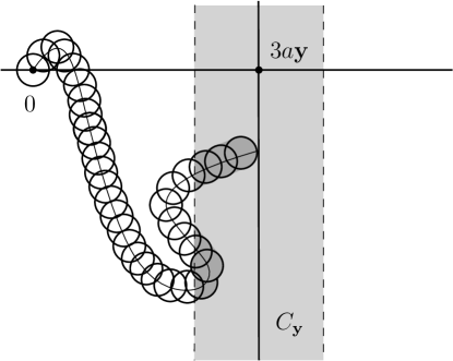
Suppose for now that . Let . With a standard Brownian motion on with , let be the corresponding Wiener sausage (3.40). We explain next the state open/closed for a vertex . Let
| (3.49) |
Since is recurrent, we have a.s. Let be the lifetime of , and define the event
| (3.50) |
We explain next how is chosen (see Figure 3.1). Let and, for , consider the intersection
Lemma 3.15.
There exists such that the volume of satisfies
Proof.
The set is the union of disjoint subsets of the Wiener sausage, exactly one of which, denoted , touches the line . The volume of is bounded below by the volume of the union of a cylinder with radius and length , and a half-sphere with radius . Thus,
whence the lemma holds with . ∎
By Lemma 3.15, we may pick sufficiently large that
If , we pick the least point in the intersection (in lexicographic order) and denote it , and we say that has been occupied from . We call open if occurs, and closed otherwise.
By the recurrence of , we may choose such that, for ,
| (3.51) |
In order to define the open/closed states of other , it is necessary to generalize the above slightly, and we do this next. Instead of considering a Brownian motion starting at , we move the starting point to some . Thus becomes , and (3.49)–(3.50) become
By the recurrence of , we may choose such that
| (3.52) |
The extra notation introduced above will be used at the next stage.
We construct a non-decreasing sequence pair of disjoint subsets of in the following way. The set is the set of vertices known to be open at stage of the construction, and is the set known to be closed. Our target is to show that the dominate some supercritical percolation process.
The vertices of are ordered in order: for , , we declare
Let , and call the th generation of .
First, let
We choose the least , and set:
| if is open: | |||
| otherwise: |
In the first case, we say that ‘ is occupied from ’.
For , let be the set of vertices such that has some neighbour with . Suppose have been defined for , and define as follows. Select the least . If such exists, find the least such that for some . Thus is known to be open, and there exists a vertex of at the point .
As above,
If occurs we call open, and we say that is occupied from ; otherwise we say that is closed.
| If is open: | |||
| otherwise: |
By (3.51)–(3.52), the vertex under current scrutiny is open with conditional probability at least .
This process is iterated until the earliest stage at which no such exists. If this occurs for some , we declare for , and in any case we set .
The resulting set is the cluster at the origin of a type of dependent directed site percolation process which is built by generation-number. Having discovered the open vertices in generation together with the associated points , the law of the next generation is (conditionally) independent of the past and is -dependent.
We now apply a stochastic-domination argument. Such methods have been used since at least [6], and the following core lemma was systematized by Liggett, Schonmann, and Stacey [22, Thm 0.0] (see also [10, Thm 7.65] and the references therein). Let , and let be a -dependent family of Bernoulli random variables such that for all . There exists , satisfying as , such that dominates stochastically a family of independent Bernoulli variables with parameter . We choose such that exceeds the critical probability of directed site percolation on . By the above, for sufficiently small , there is strictly positive probability of an infinite directed path on comprising vertices with .
With chosen thus and , we deduce as required that . By a consideration of the geometry of the above construction, and the definition of the local states open/occupied, by (3.10) this entails .
A minor extra complication arises at the last stage, in that the events are not -dependent, but only -dependent within a given generation conditional on earlier generations. This may be viewed as follows. Begin with a family of Bernoulli variables with parameter . Having constructed the subsequence , the set (or more precisely the set of its indicator functions) dominates stochastically the th generation of . This holds inductively for all , and the claim follows.
When , we extend the earlier argument (around (3.50) and later). Rather than presenting all the required details, we consider the special case of (3.50); the general case is similar. Let and . We develop the previous reference to the first hitting time with a consideration of the limit set . Since is recurrent and is transient, there exists a deterministic such that:
-
(a)
a.s., contains infinitely many disjoint closed connected regions , each with volume exceeding , and
-
(b)
every point is such that
(3.53)
Each such region contains a point of with probability at least . Each such point is infected by with probability at least . Pick such that, in independent trials each with probability of success , there exists at least one success with probability exceeding . Finally, pick the deterministic time such that there is probability at least that contains at least disjoint closed connected regions , each with volume exceeding , and such that, for every and every , inequality (3.53) holds.
Finally, we pick such that
With these choices, the probability that contains some particle that is infected from is at least . The required argument proceeds henceforth as before.
We turn finally to the case of general and , and we indicate briefly how the method of Section 3.7.3 may be applied in the current context. First, let and . It suffices as above to show that, with probability near , infects some particle in where, as usual, . The following argument is illustrated in Figure 3.2.
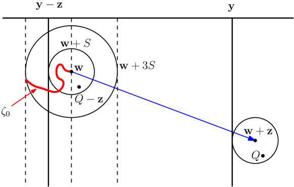
Pick and such that the version of (3.47) holds, namely,
| (3.54) |
By recurrence, the projected diffusion visits the disk infinitely often, a.s., and therefore visits the tube similarly. By the transitivity of , its entry points into are a.s. unbounded. Following each such entry to , at the point say, there is an exit from the ball . Let be the time of the first such entry and the time of the subsequent such exit.
Let denote the volume of the ball , so that
| (3.55) |
On the event that , let be the least point in that intersection, so that . Conditional on , the probability that infects the particle at during the time-interval is
| (3.56) |
By spherical symmetry and [26, Thm 3.31], conditional on ,
where is the appropriate Green’s function of [26, Lem. 3.32]. There exists such that for . We make the change of variable , and note that , to deduce that
| (3.57) |
4. The diffusion model
4.1. A condition for subcriticality
We consider the diffusion model in the general form of Sections 2.1 and 2.3, and we adopt the notation of those sections. Recall the critical point of the Boolean continuum percolation on in which a closed unit ball is centred at each point of a rate- Poisson process on . We shall prove the existence of a subcritical phase.
Condition (3.34) is now replaced as follows. Let be an independent copy of , and define the sausage
| (4.1) |
We shall assume
| (4.2) | C: for , , |
for some , and we make a note about this condition in Remark 4.3.
Let be the probability that the diffusion process survives.
Theorem 4.1.
Consider the general diffusion model on where .
-
(a)
Let and . Then if .
-
(b)
Let and . Assume in addition that condition C of (4.2) holds. Let and . Then if and .
This theorem extends Theorem 1.2. Its proof is related to that given in Section 3.4 for the delayed diffusion model.
Proof.
(a) Let , and suppose that . We shall enhance the probability space on which the diffusion model is defined. Let be random variables with the exponential distribution with parameter ; these are independent of one another and of all other random variables so far. We call the ‘lifetime’ of , and it is the length of the period between infection and removal of .
For , we introduce Poisson processes of points in , and we say that ‘contacts’ at the times of . The intensity functions of the depend as follows on the positions of and . Conditional on and the diffusions , let be independent Poisson processes on with respective rate functions
The points of are denoted . Let
and let be the event that and is susceptible at all times for . Suppose that becomes infected at time . The first contact by of after time results in an infection if and only the event occurs (in which case we say that infects directly). Write and .
Proposition 3.7 holds with the same proof but with replaced by
| (4.3) |
where is an independent copy of . By the Poisson colouring theorem, equals the probability that contacts a particle started at during the time interval . With this new , the new bound now satisfies
| (4.4) |
In other words, is the mean number of particles that contacts during its lifetime (it is not the mean total number of contacts by , since may contact any given particle many times).
By an inductive definition as before, we define the th generation of infected particles from . We claim that
| (4.5) |
By (4.5), whenever , and the claim of part (a) follows by (4.4) as in the proof of Proposition 3.8(b, c). We turn therefore to the proof of (4.5), which we prove first with .
Recall that each label corresponds to a point , an associated diffusion , and a lifetime . The lifetime is the residual time to removal of after its first infection.
Suppose next that . We introduce some further notation. Let , and let be an ordered vector of distinct members of ; we shall consider as both a vector and a set. Define the increasing sequence of times by
| (4.8) |
By iterating the argument leading to (4.6), we obtain
| (4.9) |
where
| (4.10) |
and
| (4.11) |
Equations (4.9)–(4.10) are implied by the following observation: if , then there exists a sequence such that, for , infects directly at the time . See Figure 4.1.

By (4.10),
where and is the -field generated by the random variables
Note that are -measurable, so that
Therefore,
| (4.12) |
where the summations are over distinct .
It is tempting to argue as follows. The diffusions are independent of , and is -measurable. By the Poisson displacement theorem (see [20, Sec. 5.2]), the positions are a subset of a rate- Poisson process. It follows that
| (4.13) |
| (4.14) |
Inequality (4.5) follows by iteration and (4.9) There is a subtlety in the argument leading to (4.13), namely that the distribution of the subset of will generally depend on the choice of . This may be overcome as follows.
We decouple the indices of particles and their starting positions in a classical way (see [12, Thm 6.13.11]) by giving a more prescriptive recipe for the construction of the Poisson process . Let be a positive integer and let ; later we shall take the limit as . Let have the Poisson distribution with parameter . Conditional on , let be independent random variables with the uniform distribution on . Thus, points in are indexed where , with retaining the index .
Let
| (4.15) |
so that as , and furthermore,
| (4.16) |
by the monotone convergence theorem. The sum may be represented in terms of the average of where is a random ordered -subset of indices in , namely,
| (4.17) |
The term is intepreted as if . With and , we have as in (4.12) that
| (4.18) |
where
| (4.19) |
and .
For an ordered -subset of , let be the supremum over of the mean number of particles infected by a given initial particle located at , in the subset of the rate- Poisson process obtained from by deleting . Note that
| (4.20) |
By (4.16), on letting , we deduce inequality (4.14), and the proof is completed as before.
(b) Let . We repeat the argument in the proof of part (a) (cf. Section 3.6) with defined as the mean number of particles for which there exists with . That is, with an independent copy of ,
| (4.21) | ||||
where is given in (4.1). As in Theorem 3.10(b) adapted to the diffusion model, we have by C that if and . By the argument of the proof of part (a), for and . ∎
Example 4.2 (Bounded motion).
Remark 4.3 (Condition C).
Let , the maximum displacement of up to time , and let be given similarly in terms of . By Minkowski’s inequality,
Here, denotes the norm. Therefore, C holds for some , if for suitable , .
4.2. The Brownian diffusion model
Suppose that , , and is a standard Brownian motion (one may allow it to have constant non-zero drift, but for simplicity we set the drift to ). Since is a standard Brownian motion, it is easily seen that where is the usual radius- Wiener sausage. Therefore,
Hence, where is the corresponding quantity of Example 3.13 for the delayed diffusion model.
4.3. Survival
We close with some remarks on the missing ‘survival’ parts of Theorems 1.2 and 4.1. An iterative construction similar to that of Section 3.7 may be explored for the diffusion model. However, Proposition 3.3 is not easily extended or adapted when the particles are permanently removed following infection.
The situation is different when either there is no removal (that is, , see [3]), or ‘recuperation’ occurs in that particles become susceptible again post-infection. A model of the latter type, but involving random walks rather than Brownian motions, has been studied by Kesten and Sidoravicius in their lengthy and complex work [18]. Each of these variants has structure not shared with our diffusion model, including the property that the set of infectives increases when the set of initially infected particles increases. Heavy use is made of this property in [18]. Unlike the delayed diffusion model (see the end of Section 3.1 and Proposition 3.4), neither the diffusion model nor its random-walk version has this property, in contradiction of the claim of Remark 4 of [18].
Acknowledgements
ZL’s research was supported by National Science Foundation grant 1608896 and Simons Foundation grant 638143. GRG thanks Alexander Holroyd and James Norris for useful conversations. The authors are very grateful to three referees for their detailed and valuable reports, which have led to significant corrections. The work reported here was influenced in part by the Covid-19 pandemic of 2020.
References
- [1] O. S. M. Alves, F. P. Machado, and S. Yu. Popov, Phase transition for the frog model, Electron. J. Probab. 7 (2002), paper no. 16, 21 pp. MR 1943889
- [2] by same author, The shape theorem for the frog model, Ann. Appl. Probab. 12 (2002), 533–546. MR 1910638
- [3] E. Beckman, E. Dinan, R. Durrett, R. Huo, and M. Junge, Asymptotic behavior of the Brownian frog model, Electron. J. Probab. 23 (2018), paper no. 104, 19 pp. MR 3870447
- [4] I. Benjamini, L. R. Fontes, J. Hermon, and F. P. Machado, On an epidemic model on finite graphs, Ann. Appl. Probab. 30 (2020), 208–258. MR 4068310
- [5] J. van den Berg, R. Meester, and D. G. White, Dynamic Boolean models, Stoch. Proc. Appl. 69 (1997), 247–257. MR 1472953
- [6] J.-D. Deuschel and A. Pisztora, Surface order large deviations for high-density percolation, Probab. Theory Related Fields 104 (1996), 467–482. MR 1384041
- [7] L. R. Fontes, F. P. Machado, and A. Sarkar, The critical probability for the frog model is not a monotonic function of the graph, J. Appl. Probab. 41 (2004), 292–298. MR 2036292
- [8] R. K. Getoor, Some asymptotic formulas involving capacity, Z. Wahrsch’theorie und verwandte Gebiete 4 (1965), 248–252. MR 190988
- [9] P. Gracar and A. Stauffer, Percolation of Lipschitz surface and tight bounds on the spread of information among mobile agents, Approximation, Randomization, and Combinatorial Optimization. Algorithms and Techniques, LIPIcs, Leibniz Int. Proc. Inform., vol. 116, Schloss Dagstuhl. Leibniz-Zent. Inform., Wadern, 2018, paper 39. MR 3857277
- [10] G. R. Grimmett, Percolation, 2nd ed., Grundlehren der Mathematischen Wissenschaften, vol. 321, Springer-Verlag, Berlin, 1999. MR 1707339
- [11] by same author, Probability on Graphs, 2nd ed., Cambridge University Press, Cambridge, 2018. MR 3751350
- [12] G. R. Grimmett and D. R. Stirzaker, Probability and Random Processes, 4th ed., Oxford University Press, Oxford, 2020. MR 4229142
- [13] Y. Hamana and H. Matsumoto, A formula for the expected volume of the Wiener sausage with constant drift, Forum Math. 29 (2017), 369–381. MR 3619119
- [14] P. H. Haynes, V. H. Hoang, J. R. Norris, and K. C. Zygalakis, Homogenization for advection–diffusion in a perforated domain, Probability and Mathematical Genetics, vol. 37, Cambridge University Press, 2010, pp. 397–415. MR 2744249
- [15] C. Hoffman, T. Johnson, and M. Junge, Cover time for the frog model on trees, Forum Math. Sigma 7 (2019), Paper No. e41, 49 pp. MR 4031108
- [16] T. Johnson and M. Junge, Stochastic orders and the frog model, Ann. Inst. Henri Poincaré Probab. Stat. 54 (2018), 1013–1030. MR 3795075
- [17] H. Kesten and V. Sidoravicius, The spread of a rumor or infection in a moving population, Ann. Probab. 33 (2005), 2402–2462. MR 2184100
- [18] by same author, A phase transition in a model for the spread of an infection, Illinois J. Math. 50 (2006), 547–634. MR 2247840
- [19] by same author, A shape theorem for the spread of an infection, Ann. of Math. (2) 167 (2008), 701–766. MR 2415386
- [20] J. F C. Kingman, Poisson Processes, Oxford Studies in Probability, vol. 3, Oxford University Press, Oxford, 1993. MR 1207584
- [21] K. Kuulasmaa, The spatial general epidemic and locally dependent random graphs, J. Appl. Probab. 19 (1982), 745–758. MR 675138
- [22] T. M. Liggett, R. H. Schonmann, and A. M. Stacey, Domination by product measures, Ann. Probab. 25 (1997), 71–95. MR 1428500
- [23] C. Marinelli and M. Röckner, On the maximal inequalities of Burkholder, Davis and Gundy, Exposit. Mathem. 34 (2016), 1–26. MR 3463679
- [24] P. Mattila, Geometry of Sets and Measures in Euclidean Spaces, Cambridge University Press, Cambridge, 1995. MR 1333890
- [25] R. Meester and R. Roy, Continuum Percolation, Cambridge Tracts in Mathematics, vol. 119, Cambridge University Press, Cambridge, 1996. MR 1409145
- [26] P. Mörters and Y. Peres, Brownian Motion, Cambridge Series in Statistical and Probabilistic Mathematics, vol. 30, Cambridge University Press, Cambridge, Cambridge, 2010. MR 2604525
- [27] Y. Peres, A. Sinclair, P. Sousi, and A. Stauffer, Mobile geometric graphs: Detection, coverage and percolation, Probab. Theory Related Fields 156 (2013), 273–305. MR 3055260
- [28] S. Yu. Popov, Frogs and some other interacting random walks models, Discrete Random Walks, Assoc. Discrete Math. Theor. Comput. Sci., Nancy, 2003, pp. 277–288. MR 1819703
- [29] A. F. Ramírez and V. Sidoravicius, Asymptotic behavior of a stochastic growth process associated with a system of interacting branching random walks, C. R. Math. Acad. Sci. Paris 335 (2002), 821–826. MR 1947707
- [30] L. T. Rolla, Activated random walks on , Probab. Surveys 17 (2020), 478–544. MR 4152668
- [31] L. T. Rolla, V. Sidoravicius, and O. Zindy, Universality and sharpness in activated random walks, Ann. Henri Poincaré, Theor. & Math. Phys. 20 (2019), 1823–1835. MR 3956161
- [32] F. Spitzer, Electrostatic capacity, heat flow and Brownian Motion, Z. Wahrsch’theorie und verwandte Geb. 3 (1964), 110–121. MR 172343
- [33] A. Stauffer and L. Taggi, Critical density of activated random walks on transitive graphs, Ann. Probab. 46 (2018), 2190–2220. MR 3813989