BSDA: Bayesian Random Semantic Data Augmentation for Medical Image Classification
Abstract
Data augmentation is a crucial regularization technique for deep neural networks, particularly in medical image classification. Mainstream data augmentation (DA) methods are usually applied at the image level. Due to the specificity and diversity of medical imaging, expertise is often required to design effective DA strategies, and improper augmentation operations can degrade model performance. Although automatic augmentation methods exist, they are computationally intensive. Semantic data augmentation can implemented by translating features in feature space. However, over-translation may violate the image label. To address these issues, we propose Bayesian Random Semantic Data Augmentation (BSDA), a computationally efficient and handcraft-free feature-level DA method. BSDA uses variational Bayesian to estimate the distribution of the augmentable magnitudes, and then a sample from this distribution is added to the original features to perform semantic data augmentation. We performed experiments on nine 2D and five 3D medical image datasets. Experimental results show that BSDA outperforms current DA methods. Additionally, BSDA can be easily assembled into CNNs or Transformers as a plug-and-play module, improving the network’s performance. The code is available online at https://github.com/YaoyaoZhu19/BSDA.
Data Augmentation, Medical Image, Variational Bayesian
1 Introduction
Deep learning methods can assist clinicians in rapid examination and accurate diagnosis [1]. However, these methods are data-demanding, and medical images are often scarce. For example, insufficient patients with specific diseases or a lack of medical equipment can lead to biased, overfitting, and inaccurate models [1]. Data augmentation is a common regularization technique to address these issues [2, 3]. The variety of medical image modalities (e.g., MR, CT, X-ray, Retina) and their association with different clinical diseases necessitate specialized knowledge and careful debugging for image-level data augmentation methods to improve network performance significantly. Although automated data augmentation methods [4, 5] can avoid manual debugging, they are computationally expensive. Additionally, image-level data augmentation methods often need help to improve sample diversity and achieve semantic transformations. While generative data augmentation methods [6, 7, 8, 9] can enhance semantic diversity, they are also computationally expensive and complex to train, making them challenging for medical practitioners without a computer science background.
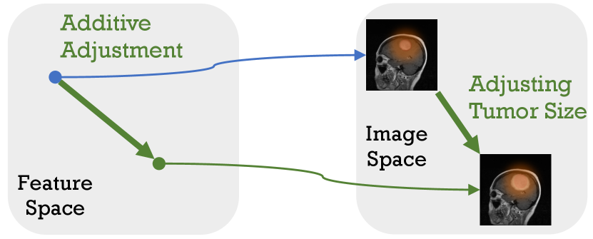
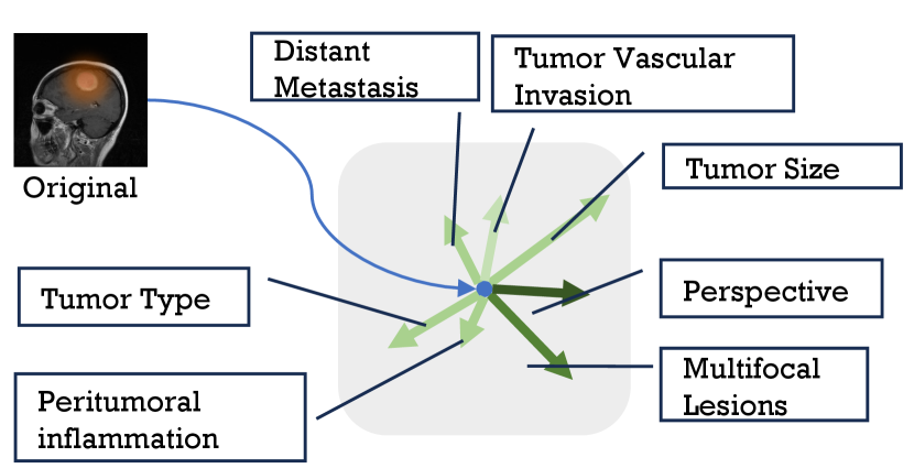
Recent studies have shown that feature-level data augmentation methods can enhance network performance [10, 11, 12, 13]. In detail, the deep feature space harbors various semantic directions, and translating features along these directions yields new sample features with identical class identities but alter semantic content [14]. An example is shown in Figure 1, subfigure 1(b) shows different semantic directions in feature space of original image input to the deep network, and subfigure 1(a) shown translate deep feature along ‘tumor size,‘ we will then obtain the depth features of another image where the tumor size has changed but maintained other semantics.
The ISDA [14] stands out in this domain, facilitating implicit data augmentation by aiming to minimize an upper bound of the expected cross-entropy loss on the augmented dataset. Unlike traditional methods that modify images directly, this approach generates new data at the feature level, such as operating random disturbances, interpolations, or extrapolations within the feature space for augmentation [15]. In medical images, there are numerous modalities with non-uniform dimensions. data augmentation methods based on image transformations provide limited enhancement of diversity, and computational cost of generative data augmentation methods is high, the generative data augmentation methods are computationally costly, although they can enrich diversity Semantic data augmentation holds promise in addressing the shortcomings of both approaches. Current semantic data augmentation methods [14, 16] mainly aim to improve the semantic direction, whereas semantic strength should be equally important because over-translation may violate the image label.
To address this issue and develop a universal semantic augmentation paradigm for medical image classification, we drew inspiration from the automatic augmentation method: RA [5], defining a semantic data augmentation strategy incorporating two hyperparameters: semantic magnitude and semantic direction. Inspired by the concept that modeling data augmentation as additive perturbation can enhance network learning and generalization capabilities [17], we define a semantic data augmentation method as the addition of semantic magnitude to the original feature in selected semantic directions. For example, in the tumor staging task, a feature represents the semantics of tumor size, and we change the tumor size by changing the feature value.
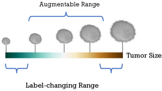
However, Figure 2 shows that alterations beyond the permissible range within the category may result in label changes. Therefore, we treat the augmentable (label-preserving) semantic magnitude as a random variable and estimate its distribution using variational Bayesian. For semantic directions, similar to the image space augmentation approache [18], it is a naive idea to select semantic directions randomly, but it does not make sense to perform augmentation in certain directions [14], a view based on image space. Some data augmentation approaches [19, 20] are adequate for downstream tasks, although they do not make sense vision, and the quantitative evaluation approaches proposed in [21] explain why vision meaningless data augmentation approaches are still practical. Not coincidentally, [12] point out that adding a random Gaussian perturbation to the features significantly improves the Empirical Risk Minimization (ERM), although it does not follow any meaningful direction. Even the perturbation of randomness due to the reparameterization introduced by variational inference benefits the network’s learning of features [12]. Therefore, we do not augment all directions but randomly select semantic directions like the random selection transform in image space.
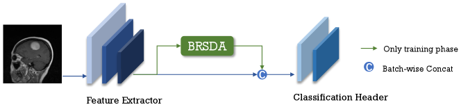
In summary, we propose a simple yet efficient feature-level method for semantic data augmentation called Bayesian Random Semantic Data Augmentation (BSDA). BSDA adds semantic magnitudes to randomly selected directions, with the magnitudes obtained by sampling from augmentable semantic magnitude distribution estimated using variational inference. Figure 3 shows BSDA inserted into the network as a plug-in. Our main contributions are:
-
•
We propose a high-performance Bayesian random semantic data augmentation plug-and-play module, BSDA, for medical image classification.
-
•
We experimentally demonstrate that BSDA outperforms current data augmentation methods.
-
•
We provide experimental evidence demonstrating that BSDA can enhance network performance across different dimensions, modalities, and neural network architectures, including both CNNs and Transformers.
2 Related Work
2.1 Data Augmentation
In image recognition tasks, data augmentation techniques like random flipping, panning, and rotation make the network learn certain invariants [18, 22]. These methods rely heavily on empirical knowledge, and a specific augmentation strategy can only be used for a particular dataset. AutoAugment [4] was the first technique to perform automatic augmentation by searching for a better strategy across numerous solution spaces using reinforcement learning. However, due to the large of its search space, other works (e.g., RA [5], DADA [23]) have also shown strong performance by improving the search algorithm. While automated data augmentation algorithms have shown strong capabilities, the training of deep neural networks remains computationally intensive. Image Erasure [24] and Image Mixing [25, 19, 20] enhance the performance of the network by performing random erasure or mixing of images in the image space. Generative models have also shown strong performance in image generation, with some works [26, 27] developing data augmentation techniques based on image generation. However, these methods require additional training of a generative model for each dataset. A Bayesian data augmentation method proposed in [28] learns the distribution of features from the training set by generating an adversarial network implementing generalized Monte Carlo expectation maximization and samples from it to obtain augmented data. It is worth noting that our method is similar in name but differs in approach. Several studies have explored the efficiency of data augmentation. [17] notes that data augmentation modeled as additive perturbation improves network performance by amplifying and perturbing the singular values of the network’s Jacobian determinant. Similarly, [29] showed a lower bound on the data required for data augmentation, demonstrating that the general use of DA requires an exponential amount of data before it leads to larger bounds.
2.2 Semantic Data Augmentation
Semantic data augmentation is achieved by label-preserving translation in the semantic space, generating new sample points in the feature space. Three semantic augmentation schemes involve adding random Gaussian noise with mean 0 and variance to the features, interpolating neighbors, and extrapolating [15]. Similarly, OnlineAugment [30] achieves excellent performance by using Gaussian noise to perturb features, but it tends to generate non-class-preserving sample points. Furthermore, [16] used a moving average to estimate the feature covariance matrix online during training and modeled the cross-feature joint noise distribution. ISDA [14] is a novel semantic data augmentation algorithm that enhances dataset diversity by translating training samples in the deep feature space along semantically meaningful directions, improving the generalization performance of deep models with minimal computational cost. A shape space-based feature augmentation method projects multiple image features into a pre-shape space. [31] uses Wasserstein geodesic interpolation to augment data and regularize performance. Moment Exchange is an implicit data augmentation method that enhances recognition models by replacing and interpolating learned features’ moments (mean and standard deviation) between training images. This forces models to extract training signals from these moments, thus improving generalization across benchmark datasets [32].
3 Method
Consideraing training a deep neural network included two parts: a feature extraction network and a classification network with parameters on a dataset , where each represents a label belonging to one of classes. The output of is a dimensions feature vector , which is then input into to predict the target , where is the predicted class label. We refer to as the original feature vector for clarity.
3.1 BSDA
The BSDA method generates augmented feature by adding the semantic magnitude to the original feature after element-wise multiplication of them with randomly selected semantic directions . The formula is as follows:
| (1) |
where is a binary vector, initially set to all ones and then set to zero with probability , and denotes element-wise multiplication. represents the semantic magnitude sampled from the augmentable magnitude distribution when given the original feature vector . Furthermore, to preserve specific properties of the features, such as low rank [33, 34, 35], we mask semantic directions corresponding to zero feature values. We have:
| (2) |
where is an indicator function when , the value of this function is 1.
Estimate the magnitude distribution. To obtain , we introduce a model to approximate the true distribution . The Kullback-Leibler (KL) divergence measures the similarity between these two distributions, aiming to make closely match by maximizing the KL divergence. Thus, our optimization goal is as follows:
| (3) |
Removing the terms that are not related to the parameter in , we have:
| (4) | ||||
Loss function of BSDA. The first term of Eq. 4 can be calculated easily. The second term estimates the features given , which is more challenging to compute. Drawing inspiration from the design of Variational Autoencoders (VAE) [36], we introduce a reconstruction network for learning this term, rewriting the second term as . Then, we obtain the loss function of BSDA as follows:
| (5) | ||||
The second part of Eq. 5 depends on the model, and we use MSE loss in BSDA. Assuming the marginal distribution follows a normal distribution and also follows a normal distribution , setting the mean to zero because we aim to learn the offset relative to the original rather than the augmented feature. Thus, the loss function of BSDA is given by:
| (6) | ||||
where is estimated variance of BSDA, and is reconstructed feature using .
The reparameterization trick. We employ the reparameterization trick to facilitate the computation of the loss function while ensuring the gradient flow for effective backpropagation. The random variable can be represented as a deterministic variable , with being an auxiliary variable with an independent marginal distribution , and being a vector-valued function parameterized by .
Loss function. Our augmentation method is training with . For convenience, we denote the loss of as , which typically uses cross-entropy loss in classification tasks. Therefore, the total loss function is:
| (7) |
Different superscripts on distinguish between augmented and original features. The hyperparameter is a dynamic value introduced to mitigate the impact of BSDA on the network during the initial stages of training when the network has yet to learn valuable features.
To summarize, the BSDA technique can be integrated into deep networks. We provide the pseudocode of BSDA in Algorithm 1.
3.2 Compare with other methods
VAE. Our approach resembles VAE [36], where a latent variable is estimated and used for reconstruction. However, the relationship between our latent variable and the inputs differs from VAE [36], the latent variable representation of the inputs in VAE [36]. Our latent variable represents the augmentable range in a given feature without altering the label.
ISDA. Our approach differs from ISDA [14] in several key aspects: (a) it does not depend on the task’s loss function; (b) it serves as an implicit data augmentation method, complementing the explicit ISDA. This makes BSDA more convenient for special treatments in particular network branches. For instance, the BSDA module can be applied to both branches simultaneously in feature-decoupled networks, achieving post-decoupled feature enhancement.
4 Experiments
In this section, we empirically validate the proposed algorithm on MedMNIST+ [37], a large-scale collection of standardized biomedical images. Our evaluation strategy encompassed several vital aspects: comparison with state-of-the-art methods, effectiveness across modalities and dimensions, and adaptability to different neural network architectures. Finally, we performed ablation experiments, hyperparameter analysis, and visualization of deep features.
4.1 Datasets and Training Details
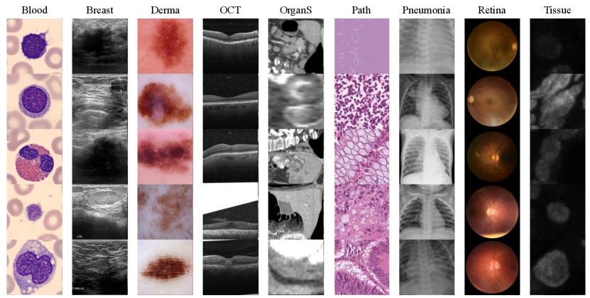
Dataset. The MedMNIST+ [37] dataset comprises twelve pre-processed 2D datasets and six pre-processed 3D datasets from selected sources covering primary data modalities (e.g., X-ray, OCT, Ultrasound, CT, Electron Microscope), diverse classification tasks (binary/multi-class, ordinal regression, and multi-label) and data scales (from 100 to 100,000) [37]. We selected nine 2D medical image datasets and six 3D medical image datasets in MedMNIST+ [37] covering twelve modalities, as shown in Figure 4. For more details on the dataset, please refer to Table 1.
Dataset Data Modality Tasks (Classes/Labels) Samples Training/Validation/Test Blood Blood Cell Microscope Multi-Class (8) 17,092 11,959 / 1,712 / 3,421 Breast Breast Ultrasound Binary-Class (2) 780 546 / 78 / 156 Derma Dermatoscope Multi-Class (7) 10,015 7,007 / 1,003 / 2,005 OCT Retinal OCT Multi-Class (4) 109,309 97,477 / 10,832 / 1,000 OrganS Abdominal CT Multi-Class (11) 25,211 13,932 / 2,452 / 8,827 Path Colon Pathology Multi-Class (9) 107,180 89,996 / 10,004 / 7,180 Pneumonia Chest X-Ray Binary-Class (2) 5,856 4,708 / 524 / 624 Retina Fundus Camera Ordinal Regression (5) 1,600 1,080 / 120 / 400 Tissue Kidney Cortex Microscope Multi-Class (8) 236,386 165,466 / 23,640 / 47,280 Organ3D Abdominal CT Multi-Class (11) 1,742 971/161/610 Nodule3D Chest CT Binary-Class (2) 1,633 1,158/165/310 Adrenal3D Abdominal CT Binary-Class (2) 1,584 1,188/98/298 Fracture3D Chest CT Multi-Class (3) 1,370 1,027/103/240 Vessel3D Brain MRA Binary-Class (2) 1,908 1,335/191/382
Evaluation Protocols We used the MedMNIST+ split training set and validation set to select hyperparameters and reported the results of the test set. The Randomness arising from model selection is often ignored. For instance, does method A outperform method B only because the random search for A got lucky [38]? Therefore, we repeated the process three times with different random seeds. Every number we report is the mean of these repetitions and their estimated standard error. The area under the ROC curve (AUC) and accuracy (ACC) are used as the evaluation metrics.
Implementation Details. We implemented BSDA using PyTorch 2.2.2 and Torchvision 0.17.2 and experimented on an NVIDIA RTX 4090 GPU with an Intel 14900k CPU. During training, we utilized the AdamW [39] optimizer with a learning rate of 0.001 and employed a learning rate warm-up strategy for the first five epochs. The 2D image size is , and the 3D image size is . To ensure fairness, we maintained consistent training configurations across all experiments. The distribution estimator and reconstruction modules of BSDA consist of two fully connected layers, followed by BatchNorm and GeLU activation.
4.2 Comparison Experiment
First, we evaluated state-of-the-art methods on nine 2D medical image datasets in MedMNIST2D [37](BloodMNIST, BreastMNIST, DermaMNIST, OCTMNIST, OrgansMNIST, PathMNIST, PneumoniaMNIST, RetinaMNIST, and TissueMNIST), which include a total of 513,429 samples. We compared BSDA with state-of-the-art methods, including Cutout [40], Mixup [25], CutMix [20], and ISDA [14]., on nine 2D medical image datasets.
Method Blood Breast Derma OCT OrganS Path Pneumonia Retina Tissue Avg Official Baseline Mixup Cutout CutMix ISDA BSDA(Our)
Method Blood Breast Derma OCT OrganS Path Pneumonia Retina Tissue Avg Official Baseline Mixup Cutout CutMix ISDA BSDA(Our)
4.2.1 ACC Results of MedMNIST2D+
Table 2 reveals that BSDA is the top-performing method, achieving the highest average accuracy of 81.9% across all evaluated datasets. ISDA also performs strongly with an average accuracy of 81.0%, but is slightly less consistent than BSDA. This demonstrates the advantages of semantic data augmentation methods for medical images and highlights that BSDA outperforms ISDA. For example, BSDA achieved 70.4% accuracy on TissueMNIST and 82.2% on OrgansMNIST, while ISDA achieved 68.1% and 80.8% on these datasets, respectively. Methods like CutMix [20], CutOut [40], and MixUp [25] offer comparable results, with average accuracies of 80.4%, 80.8%, and 80.1%, respectively, yet none consistently surpass the performance of ISDA and BSDA. RetinaMNIST is the most challenging dataset, with all methods showing lower accuracy levels around 50-53%, such as ISDA at 52.6% and BSDA at 53.3%. The results highlight the critical role of data augmentation techniques in enhancing model performance, as the baseline consistently underperforms with an average accuracy of 79.0%, emphasizing the necessity of employing sophisticated augmentation strategies in medical imaging tasks.
4.2.2 AUC Results of MedMNIST2D+
The results of Table 3 reinforces the effectiveness of BSDA, which not only achieves the highest average AUC but also consistently performs across different datasets. BSDA achieves an average AUC of 93.9%, indicating its effectiveness in enhancing the model’s ability to distinguish between classes. This performance is slightly higher than other methods. BSDA exhibits lower variability in performance across most datasets, indicating more consistent results. For instance, its standard deviation in AUC is relatively low, especially compared to methods like Mixup [25] and ISDA [14], which show higher variability in datasets like PneumoniaMNIST and RetinaMNIST. ISDA and CutMix [20] also perform well but with higher variability. BSDA consistently outperforms other augmentation techniques in average accuracy (ACC) and area under the curve (AUC) across multiple MedMNIST datasets, demonstrating superior performance and reliability in medical image classification tasks.
4.3 Results of MedMNIST3D+
We selected five 3D MedMNIST datasets to validate the performance of BSDA. As shown in Table 4. BSDA enhances the performance of ResNet-18 across various 3D datasets, with improvements in both AUC and ACC for most datasets. For example, AdernalMNIST3D shows a substantial accuracy improvement from to and a slight AUC increase from to , suggesting that BSDA significantly enhances the model’s performance, particularly in accuracy. OrganMNIST3D shows an accuracy increase from to and an AUC improvement from to . This indicates that BSDA improves the correct classification rate and enhances the model’s ability to distinguish between classes. Similarly, NoduleMNIST3D experiences a rise in accuracy from to and in AUC from to , showing consistent improvements in both metrics. For FractureMNIST3D, accuracy rises from to , while AUC improves from to . These moderate improvements indicate that BSDA helps in better identifying fractures, though the dataset remains challenging. VesselMNIST3D also benefits, with accuracy increasing from to and AUC from to , reflecting improved precision and robustness in vessel identification. These results underscore the value of data augmentation techniques in improving both the discriminative power and the accuracy of deep learning models in medical imaging tasks, demonstrating BSDA’s effectiveness in enhancing model performance across diverse medical datasets.
| Dataset | ACC% | AUC% | ||||
|---|---|---|---|---|---|---|
| Official | Baseline | BSDA(Our) | Official | Baseline | BSDA(Our) | |
| Organ3D | ||||||
| Nodule3D | ||||||
| Adernal3D | ||||||
| Fracture3D | ||||||
| Vessel3D | ||||||
| Network | ACC % | AUC % | Additional Time % | ||
|---|---|---|---|---|---|
| Baseline | BSDA | Baseline | BSDA | ||
| ResNet-18 | |||||
| ResNet-50 | |||||
| EfficientNet-B0 | |||||
| DenseNet-121 | |||||
| ViT-T | |||||
| ViT-S | |||||
| ViT-B | |||||
| Swin-T | |||||
| Swin-S | |||||
| Swin-B | |||||
4.4 Applicability of BSDA
We selected several mainstream architectures in computer vision to conduct experiments to verify the performance of BSDA combined with different models, including ResNet [18], EfficientNet [22], DenseNet [41], TinyViT [42], ViT [43], Swin Transformer [44]. Table 5 shows that the BSDA technique significantly improves accuracy (ACC) and area under the curve (AUC) across different convolutional neural networks, particularly on the DenseNet-121, ViT, and Swin Transformer series. For example, the accuracy of DenseNet-121 improved from 84.9% to 89.4%, and the AUC increased from 96.6% to 96.9%. In most cases, BSDA introduces a small additional time cost, up to 7.3% for EfficientNet-B0. Although BSDA leads to slight performance degradation on some networks (e.g., ResNet-50), overall, it improves model performance with manageable additional computational costs. Therefore, BSDA is a technique worth considering for improving model performance.
4.5 Ablation Study
| Setting | ACC% | AUC% |
|---|---|---|
| Base | ||
| BSDA | ||
| Indicator | ||
| Recon | ||
| Indicator and Recon | ||
| Random Noise | ||
| Indicator |
We analyzed the effectiveness of BSDA components and compared BSDA by adding random standard Gaussian noise to the latent space features. Table 6 indicates that random noise can somewhat improve model performance, but the improvement is limited. The BSDA model, with the introduction of the indicator function (Eq. 2) and reconstructor components, shows significant improvement over the baseline model, especially in terms of accuracy. Both the indicator function and reconstructor components are essential for BSDA. Notably, model performance degrades considerably when the indicator function and reconstructor components are removed. This is equivalent to eliminating the reconstructor as well as the second term in Eq. 5, which is comparable to simply making similar to the standard Gaussian distribution. The model performance should be comparable to that of sampling noise from a standard Gaussian distribution added to the original features, because it is simultaneously constrained by the loss of the task, thus further making the samples sampled by the model more favorable to the task.
4.6 Sensitivity Analysis
To better understand the BSDA method, we conducted a series of experiments analyzing it from different perspectives. The following sections provide a detailed analysis of the results, including hyperparameter sensitivity analysis and loss weight analysis.
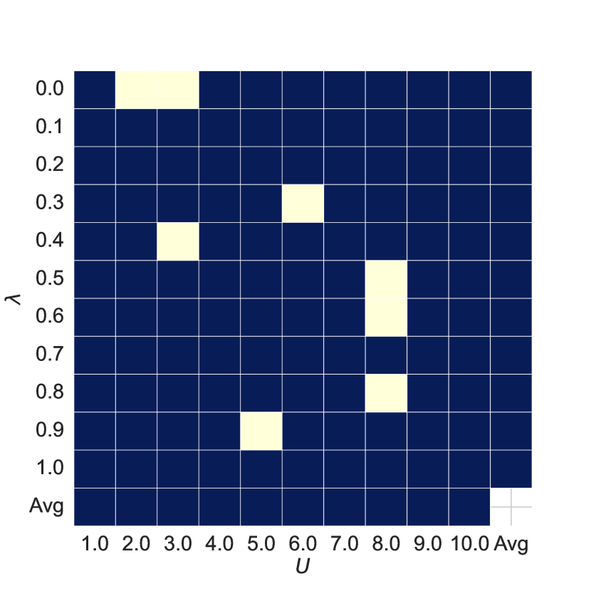
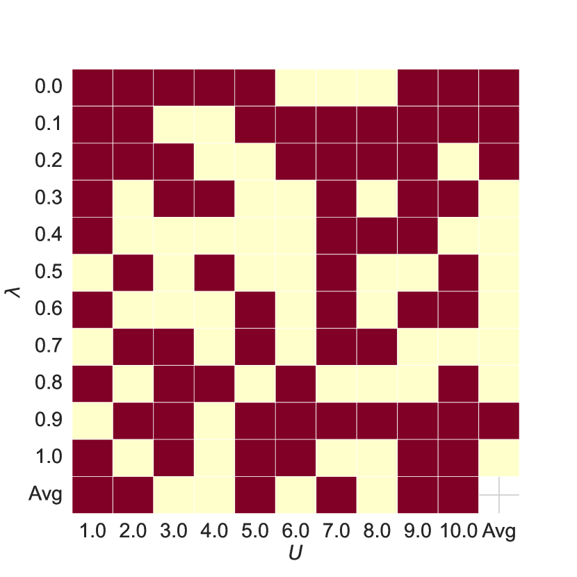
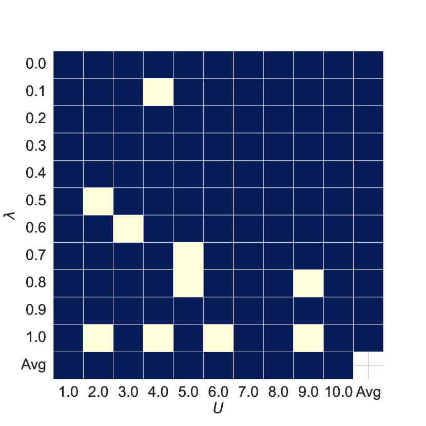
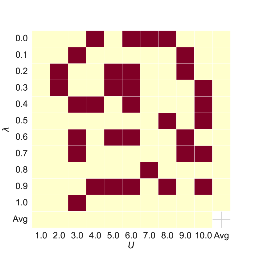
Hyper-parameters Analysis As shown in Figure 5, subplots 5(a) and 5(b) show the AUC and ACC results of the joint features for different hyperparameters and compared to the baseline, with red or blue indicating improvements over the baseline. Comparing subplots 5(a) and 5(c) and 5(b) and 5(d), we see that the joint features improve model performance in most cases.
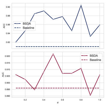
Weight of Loss We conducted a sensitivity analysis of the hyperparameter of BSDA using ResNet-18 on the BreastMNIST dataset. The results are shown in Figure 6. We chose the hyperparameter values from 0.1 to 1. It can be observed that the AUC and ACC metrics are stable in almost all cases, indicating that the BSDA method is not sensitive to the hyperparameter . The AUC value is slightly lower than the baseline at or , and the ACC value is somewhat lower than the baseline at or . Empirically, we recommend as the default parameter.
4.7 Visualization of Deep Features
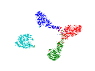
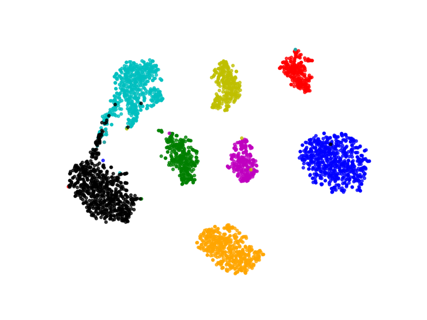
We visualize the deep features using t-SNE [45] in Figure 7. Circular markers represent the original features, while the cross markers indicate the augmented features generated by BSDA. The results show that the augmented features are distributed around the original features, indicating that BSDA generates augmented features that are close to the original ones. Figure 7 also shows that the original features wrap tightly around the newly generated features. Intuitively, classifiers learned from the augmented features will be farther from the original features.
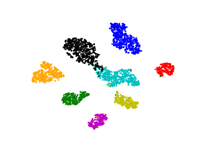
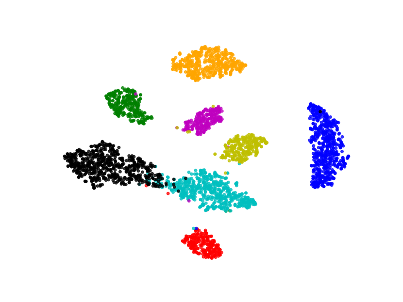
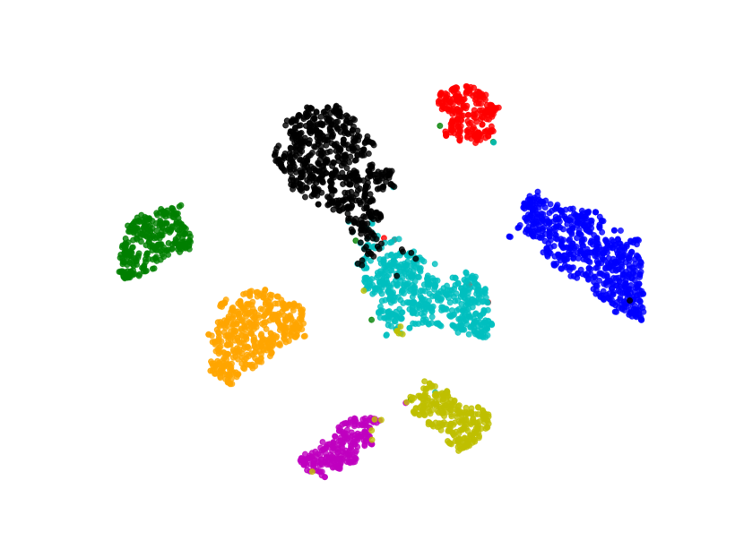
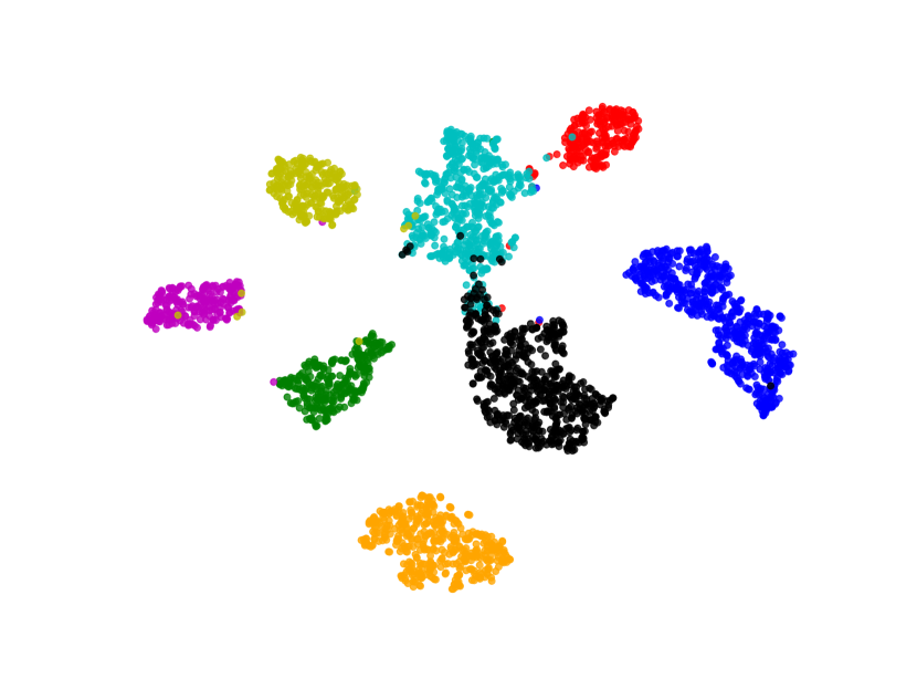
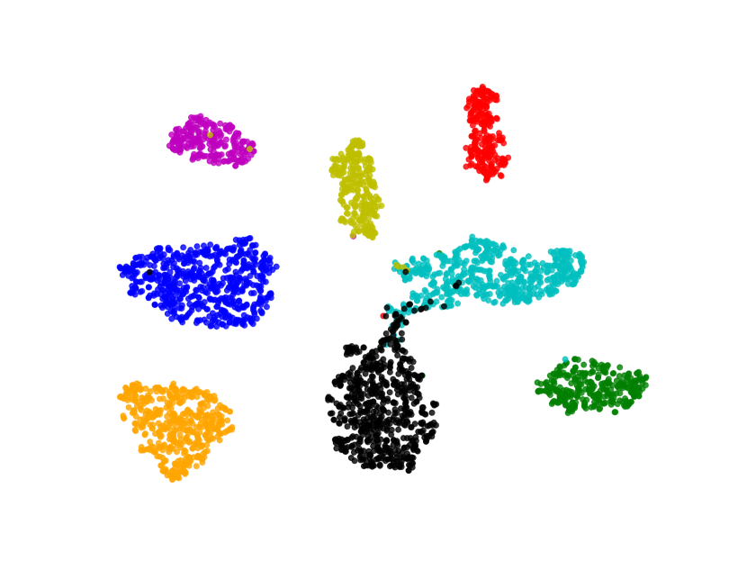
We also visualize the features learned by our method compared to other methods (without feature-level or image-level augmentation). Figure 8 shows that BSDA methods (Fig. 8(f)) make the intra-class features more cohesive and more easily separable.
5 Discussion
BSDA, as an explicit data augmentation method, has many promising applications in medical imaging. For example, in the case of multimodal or multiparametric medical images, BSDA can be flexibly inserted into the network as a plug-in to provide semantic data augmentation for different modalities simultaneously, potentially enhancing the model’s performance. Another example is the multicenter setting, typical in medical imaging, where the model must be generalized to other domains. Some methods use feature decoupling-based or feature disentanglement-based domain generalization. BSDA can also provide semantic data augmentation for different decoupled branches, potentially enhancing the model’s generalization ability. Moreover, medical image datasets often need to be more balanced. Adding a balanced sampling strategy during data augmentation in the training phase can improve network performance on unbalanced datasets.
BSDA presents a versatile and efficient approach to data augmentation in medical imaging, promising significant improvements in model performance and generalization. Future work will optimize BSDA for specific medical imaging tasks and explore its potential in real-world clinical settings.
6 Conclusion
This paper introduces an efficient, plug-and-play Bayesian Random Semantic Data Augmentation (BSDA) method for medical image classification. BSDA generates new samples in feature space, making it more efficient and easy to implement. We experimentally demonstrate the effectiveness and efficiency of BSDA on various modalities, dimensional datasets, and networks.
References
- [1] E. Goceri, “Medical image data augmentation: techniques, comparisons and interpretations,” Artificial Intelligence Review, vol. 56, no. 11, pp. 12 561–12 605, Nov. 2023. [Online]. Available: https://doi.org/10.1007/s10462-023-10453-z
- [2] Z. Liu, Q. Lv, Y. Li, Z. Yang, and L. Shen, “Medaugment: Universal automatic data augmentation plug-in for medical image analysis,” ArXiv, vol. abs/2306.17466, 2023. [Online]. Available: https://api.semanticscholar.org/CorpusID:259309293
- [3] Y. N. T. Vu, R. Wang, N. Balachandar, C. Liu, A. Y. Ng, and P. Rajpurkar, “Medaug: Contrastive learning leveraging patient metadata improves representations for chest x-ray interpretation,” in Machine Learning for Healthcare Conference. PMLR, 2021, pp. 755–769.
- [4] E. D. Cubuk, B. Zoph, D. Mané, V. Vasudevan, and Q. V. Le, “Autoaugment: Learning augmentation strategies from data,” in 2019 IEEE/CVF Conference on Computer Vision and Pattern Recognition (CVPR), 2019, pp. 113–123.
- [5] E. D. Cubuk, B. Zoph, J. Shlens, and Q. V. Le, “Randaugment: Practical automated data augmentation with a reduced search space,” in 2020 IEEE/CVF Conference on Computer Vision and Pattern Recognition Workshops (CVPRW), 2020, pp. 3008–3017.
- [6] L. Chai, Z. Wang, J. Chen, G. Zhang, F. E. Alsaadi, F. E. Alsaadi, and Q. Liu, “Synthetic augmentation for semantic segmentation of class imbalanced biomedical images: A data pair generative adversarial network approach,” Computers in Biology and Medicine, vol. 150, p. 105985, 2022.
- [7] D. Li, J. Yang, K. Kreis, A. Torralba, and S. Fidler, “Semantic segmentation with generative models: Semi-supervised learning and strong out-of-domain generalization,” in Proceedings of the IEEE/CVF Conference on Computer Vision and Pattern Recognition, 2021, pp. 8300–8311.
- [8] P. A. Moghadam, S. Van Dalen, K. C. Martin, J. Lennerz, S. Yip, H. Farahani, and A. Bashashati, “A morphology focused diffusion probabilistic model for synthesis of histopathology images,” in Proceedings of the IEEE/CVF Winter Conference on Applications of Computer Vision, 2023, pp. 2000–2009.
- [9] W. H. Pinaya, P.-D. Tudosiu, J. Dafflon, P. F. Da Costa, V. Fernandez, P. Nachev, S. Ourselin, and M. J. Cardoso, “Brain imaging generation with latent diffusion models,” in MICCAI Workshop on Deep Generative Models. Springer, 2022, pp. 117–126.
- [10] E. Ahn, A. Kumar, M. Fulham, D. Feng, and J. Kim, “Unsupervised domain adaptation to classify medical images using zero-bias convolutional auto-encoders and context-based feature augmentation,” IEEE Transactions on Medical Imaging, vol. 39, no. 7, pp. 2385–2394, 2020.
- [11] Y. Kang, X. Zhao, Y. Zhang, H. Li, G. Wang, L. Cui, Y. Xing, J. Feng, and L. Yang, “Improving domain generalization performance for medical image segmentation via random feature augmentation,” Methods, vol. 218, pp. 149–157, Oct. 2023. [Online]. Available: https://www.sciencedirect.com/science/article/pii/S1046202323001329
- [12] P. Li, D. Li, W. Li, S. Gong, Y. Fu, and T. M. Hospedales, “A simple feature augmentation for domain generalization,” in 2021 IEEE/CVF International Conference on Computer Vision (ICCV), 2021, pp. 8866–8875.
- [13] M. Wang, J. Yuan, Q. Qian, Z. Wang, and H. Li, “Semantic data augmentation based distance metric learning for domain generalization,” in Proceedings of the 30th ACM International Conference on Multimedia, ser. MM ’22. New York, NY, USA: Association for Computing Machinery, 2022, p. 3214–3223. [Online]. Available: https://doi.org/10.1145/3503161.3547866
- [14] Y. Wang, G. Huang, S. Song, X. Pan, Y. Xia, and C. Wu, “Regularizing deep networks with semantic data augmentation,” IEEE Transactions on Pattern Analysis and Machine Intelligence, vol. 44, no. 7, pp. 3733–3748, 2022.
- [15] T. DeVries and G. W. Taylor, “Dataset augmentation in feature space,” arXiv preprint arXiv:1702.05538, 2017.
- [16] P. Li, D. Li, W. Li, S. Gong, Y. Fu, and T. M. Hospedales, “A simple feature augmentation for domain generalization,” in 2021 IEEE/CVF International Conference on Computer Vision (ICCV), 2021, pp. 8866–8875.
- [17] T. Y. Liu and B. Mirzasoleiman, “Data-efficient augmentation for training neural networks,” in Advances in Neural Information Processing Systems, S. Koyejo, S. Mohamed, A. Agarwal, D. Belgrave, K. Cho, and A. Oh, Eds., vol. 35. Curran Associates, Inc., 2022, pp. 5124–5136. [Online]. Available: https://proceedings.neurips.cc/paper_files/paper/2022/file/2130b8a44e2e28e25dc7d0ee4eb6d9cf-Paper-Conference.pdf
- [18] K. He, X. Zhang, S. Ren, and J. Sun, “Deep residual learning for image recognition,” in Proceedings of the IEEE conference on computer vision and pattern recognition, 2016, pp. 770–778.
- [19] D. Hendrycks, N. Mu, E. D. Cubuk, B. Zoph, J. Gilmer, and B. Lakshminarayanan, “AugMix: A simple data processing method to improve robustness and uncertainty,” Proceedings of the International Conference on Learning Representations (ICLR), 2020.
- [20] S. Yun, D. Han, S. Chun, S. J. Oh, Y. Yoo, and J. Choe, “Cutmix: Regularization strategy to train strong classifiers with localizable features,” in 2019 IEEE/CVF International Conference on Computer Vision (ICCV), 2019, pp. 6022–6031.
- [21] S. Yang, S. Guo, J. Zhao, and F. Shen, “Investigating the effectiveness of data augmentation from similarity and diversity: An empirical study,” Pattern Recognition, vol. 148, p. 110204, 2024.
- [22] M. Tan and Q. Le, “Efficientnet: Rethinking model scaling for convolutional neural networks,” in International conference on machine learning. PMLR, 2019, pp. 6105–6114.
- [23] Y. Li, G. Hu, Y. Wang, T. Hospedales, N. M. Robertson, and Y. Yang, “Differentiable automatic data augmentation,” in Computer Vision–ECCV 2020: 16th European Conference, Glasgow, UK, August 23–28, 2020, Proceedings, Part XXII 16. Springer, 2020, pp. 580–595.
- [24] Z. Zhong, L. Zheng, G. Kang, S. Li, and Y. Yang, “Random erasing data augmentation,” in Proceedings of the AAAI conference on artificial intelligence, vol. 34, no. 07, 2020, pp. 13 001–13 008.
- [25] H. Zhang, M. Cisse, Y. N. Dauphin, and D. Lopez-Paz, “mixup: Beyond empirical risk minimization,” arXiv preprint arXiv:1710.09412, 2017.
- [26] X. Zhang, Z. Wang, D. Liu, Q. Lin, and Q. Ling, “Deep adversarial data augmentation for extremely low data regimes,” IEEE Transactions on Circuits and Systems for Video Technology, vol. 31, no. 1, pp. 15–28, 2020.
- [27] H. Fang, B. Han, S. Zhang, S. Zhou, C. Hu, and W.-M. Ye, “Data augmentation for object detection via controllable diffusion models,” in Proceedings of the IEEE/CVF Winter Conference on Applications of Computer Vision (WACV), January 2024, pp. 1257–1266.
- [28] T. Tran, T. Pham, G. Carneiro, L. Palmer, and I. Reid, “A bayesian data augmentation approach for learning deep models,” Advances in neural information processing systems, vol. 30, 2017.
- [29] S. Rajput, Z. Feng, Z. Charles, P.-L. Loh, and D. Papailiopoulos, “Does data augmentation lead to positive margin?” in International Conference on Machine Learning. PMLR, 2019, pp. 5321–5330.
- [30] Z. Tang, Y. Gao, L. Karlinsky, P. Sattigeri, R. Feris, and D. Metaxas, “Onlineaugment: Online data augmentation with less domain knowledge,” in Computer Vision – ECCV 2020: 16th European Conference, Glasgow, UK, August 23–28, 2020, Proceedings, Part VII. Berlin, Heidelberg: Springer-Verlag, 2020, p. 313–329. [Online]. Available: https://doi.org/10.1007/978-3-030-58571-6_19
- [31] J. Zhu, J. Qiu, A. Guha, Z. Yang, X. Nguyen, B. Li, and D. Zhao, “Interpolation for robust learning: Data augmentation on Wasserstein geodesics,” in Proceedings of the 40th International Conference on Machine Learning, ser. Proceedings of Machine Learning Research, A. Krause, E. Brunskill, K. Cho, B. Engelhardt, S. Sabato, and J. Scarlett, Eds., vol. 202. PMLR, 23–29 Jul 2023, pp. 43 129–43 157.
- [32] B. Li, F. Wu, S.-N. Lim, S. Belongie, and K. Q. Weinberger, “On feature normalization and data augmentation,” in 2021 IEEE/CVF Conference on Computer Vision and Pattern Recognition (CVPR), 2021, pp. 12 378–12 387.
- [33] T. Galanti and T. Poggio, “Sgd noise and implicit low-rank bias in deep neural networks,” Center for Brains, Minds and Machines (CBMM), Tech. Rep., 2022.
- [34] S. R. Kamalakara, A. Locatelli, B. Venkitesh, J. Ba, Y. Gal, and A. N. Gomez, “Exploring low rank training of deep neural networks,” arXiv preprint arXiv:2209.13569, 2022.
- [35] S. Arora, N. Cohen, W. Hu, and Y. Luo, “Implicit regularization in deep matrix factorization,” Advances in Neural Information Processing Systems, vol. 32, 2019.
- [36] D. P. Kingma and M. Welling, “Auto-encoding variational bayes,” arXiv preprint arXiv:1312.6114, 2013.
- [37] J. Yang, R. Shi, D. Wei, Z. Liu, L. Zhao, B. Ke, H. Pfister, and B. Ni, “MedMNIST v2 - A large-scale lightweight benchmark for 2D and 3D biomedical image classification,” Scientific Data, vol. 10, no. 1, p. 41, Jan. 2023. [Online]. Available: https://doi.org/10.1038/s41597-022-01721-8
- [38] I. Gulrajani and D. Lopez-Paz, “In search of lost domain generalization,” in International Conference on Learning Representations, 2020.
- [39] I. Loshchilov and F. Hutter, “Decoupled weight decay regularization,” arXiv preprint arXiv:1711.05101, 2017.
- [40] T. DeVries and G. W. Taylor, “Improved regularization of convolutional neural networks with cutout,” arXiv preprint arXiv:1708.04552, 2017.
- [41] G. Huang, Z. Liu, L. Van Der Maaten, and K. Q. Weinberger, “Densely connected convolutional networks,” in Proceedings of the IEEE conference on computer vision and pattern recognition, 2017, pp. 4700–4708.
- [42] K. Wu, J. Zhang, H. Peng, M. Liu, B. Xiao, J. Fu, and L. Yuan, “Tinyvit: Fast pretraining distillation for small vision transformers,” in European Conference on Computer Vision. Springer, 2022, pp. 68–85.
- [43] A. Dosovitskiy, L. Beyer, A. Kolesnikov, D. Weissenborn, X. Zhai, T. Unterthiner, M. Dehghani, M. Minderer, G. Heigold, S. Gelly et al., “An image is worth 16x16 words: Transformers for image recognition at scale,” arXiv preprint arXiv:2010.11929, 2020.
- [44] Z. Liu, Y. Lin, Y. Cao, H. Hu, Y. Wei, Z. Zhang, S. Lin, and B. Guo, “Swin transformer: Hierarchical vision transformer using shifted windows,” in Proceedings of the IEEE/CVF international conference on computer vision, 2021, pp. 10 012–10 022.
- [45] L. Van der Maaten and G. Hinton, “Visualizing data using t-sne.” Journal of machine learning research, vol. 9, no. 11, 2008.