CAHPHF: Context-Aware Hierarchical QoS Prediction with Hybrid Filtering
Abstract
With the proliferation of Internet-of-Things and continuous growth in the number of web services at the Internet-scale, the service recommendation is becoming a challenge nowadays. One of the prime aspects influencing the service recommendation is the Quality-of-Service (QoS) parameter, which depicts the performance of a web service. In general, the service provider furnishes the value of the QoS parameters during service deployment. However, in reality, the QoS values of service vary across different users, time, locations, etc. Therefore, estimating the QoS value of service before its execution is an important task, and thus the QoS prediction has gained significant research attention. Multiple approaches are available in the literature for predicting service QoS. However, these approaches are yet to reach the desired accuracy level. In this paper, we study the QoS prediction problem across different users, and propose a novel solution by taking into account the contextual information of both services and users. Our proposal includes two key steps: (a) hybrid filtering and (b) hierarchical prediction mechanism. On the one hand, the hybrid filtering method aims to obtain a set of similar users and services, given a target user and a service. On the other hand, the goal of the hierarchical prediction mechanism is to estimate the QoS value accurately by leveraging hierarchical neural-regression. We evaluate our framework on the publicly available WS-DREAM datasets. The experimental results show the outperformance of our framework over the major state-of-the-art approaches.
Index Terms:
Hierarchical Neural-Regression, Hierarchical Prediction, Hybrid Filtering, Quality of Service (QoS) Prediction.1 Introduction
Services computing is becoming an emerging field of research with the focus shift towards Everything-as-a-Service (XaaS). With the proliferation of Internet-of-Things (IoT), Machine to Machine (M2M) communication and smart technologies, the number of web services is increasing day by day. The massive growth of the number of functionally equivalent services introduces a challenge to the service recommendation research. Numerous ways exist in the literature to recommend the services for a specific task. For example, the service recommendation can be accomplished based on user preferences [1], where the user specifies a set of criteria on which the recommender engine chooses the set of services. Sometimes, the performance of the web services becomes the principal concern, and the recommendation is made based on the QoS parameters of the services [2, 3]. Often, the cost of the services [4] is solely responsible for recommending the services. Seldom, the feature provided by the services [5] becomes the criteria for recommendation.
In this paper, we concentrate on the QoS parameters for recommending the services. The set of QoS parameters has been widely adopted to differentiate the functionally equivalent services in terms of their quality. Therefore, the QoS parameter often plays a crucial role in service recommendation. One of the fundamental challenge with QoS-based service recommendation is to obtain the exact QoS value of service before its execution. In general, the service provider supplies the QoS values of a service during its deployment. However, the QoS values of service often fluctuate depending on various factors, such as users, time, locations, etc. Therefore, determining the QoS value of service is an essential requirement, which drives our work in this paper.
A significant amount of work has been carried out in the literature to address the QoS prediction problem. One of the principal techniques for QoS prediction is collaborative filtering [6, 7, 8, 9]. The main idea of this technique is to predict the QoS value of a target service to be invoked by a user on the basis of QoS values of a set of similar services invoked by a set of similar users. The collaborative filtering is primarily of two types: memory-based and model-based. The memory-based collaborative filtering [10, 9, 11, 3, 2] is further classified into two different categories: user-based and service-based. In the user-based collaborative filtering [12], the main idea is to obtain a set of users similar to the target user before predicting the target QoS value, whereas, for the service-based collaborative filtering [13], the target QoS prediction is performed by taking into account the set of similar services. To improve the QoS prediction accuracy further, both the user-based and service-based collaborative filtering are combined to predict the target QoS value [14, 3, 6, 7, 8, 10, 2]. However, the memory-based technique suffers from the sparsity problem, which is the major limitation of this technique.
To overcome the limitation of memory-based approaches, the model-based collaborative filtering has been introduced, where different models can be learned according to the characteristics of the datasets for QoS value prediction. The matrix factorization [15, 16, 17] is one of the popular model-based QoS prediction techniques, where the QoS prediction is done based on a decomposition of a user-service matrix into low-rank matrices and followed by its reconstruction. As an improvement of matrix factorization, the regularization has been introduced further [18, 19, 20]. Regression is another approach for model-based QoS prediction [21, 22]. A few variations of regression models [23, 24] have also been proposed in this context to improve prediction accuracy. Another group of studies combined both memory-based and model-based techniques to obtain better prediction accuracy. For example, collaborative filtering can be combined with neural regression [25] to predict the target QoS value. However, the prediction accuracy is still not up to the mark, which we address in this paper.
Here, we propose a novel framework CAHPHF for QoS prediction. The crux of our proposal is to incorporate the contextual information of users and services while predicting the QoS value of a target service to be invoked by a target user. Sometimes, the contextual information carries some additional knowledge about users or services, which may be essential to improve the prediction accuracy. This fact motivates us to undertake this proposal.
Our proposed CAHPHF is a combination of memory-based and model-based techniques, and comprises two key phases: hybrid filtering followed by hierarchical prediction. In the hybrid filtering phase, we combine user-based and service-based modules by leveraging the contextual information of users or services. In the hierarchical prediction phase, we first handle the sparsity problem by filling up the matrix using collaborative filtering/matrix factorization. We then employ a hierarchical neural-regression module to predict the target QoS parameter. The hierarchical neural-regression module comprises two layers: while the first layer predicts the target QoS value, the second layer attempts to increase the prediction accuracy.
We now briefly mention the major contributions below.
(i) We present a new framework (CAHPHF) to predict the QoS value of a service to be invoked by a user while improving the prediction accuracy as compared to the state-of-the-art approaches.
(ii) Our CAHPHF, on the one hand, takes advantage of the memory-based approaches by adopting filtering. On the other hand, it leverages model-based approaches by introducing a hierarchical prediction mechanism.
(iii) We propose hybrid filtering, which is a combination of user-intensive and service-intensive filtering modules. In the user-intensive filtering module, the user is more influential than the services, whereas, in the service-intensive filtering module, the service has more impact than the user. Each of the user and service-intensive modules is again a combination of user-based and service-based filtering. Additionally, in this user/service-based filtering, we consolidate contextual information with the similarity information of the users/services intending to increase the accuracy.
(iv) A hierarchical prediction mechanism for QoS prediction is also proposed here. In this mechanism, we first focus on predicting the QoS value of the target service to be invoked by the target user. We then concentrate on reducing the error obtained by our framework.
2 Overview and Problem Formulation
In this section, we formalize our problem. We begin with defining the notion of the QoS invocation log below.
Definition 2.1.
[QoS Invocation Log:] The QoS invocation log is a 2-dimensional matrix, where each entry of the matrix represents the value of the QoS parameter of the service when invoked by the user .
It may be noted that most of the time, the QoS invocation log is a sparse matrix. If a user invoked a service in the past, the corresponding QoS value is recorded in the QoS invocation log and represented by the entry of . However, if a user never invoked a service in the past, the corresponding entry in QoS invocation log is represented by . In other words, implies the user has never invoked the service .
Example 2.1.
Consider Table I representing the QoS invocation log for a set of 10 users and a set of 10 services . Here, we consider the response time as the QoS parameter.
| 5.98 | 0.22 | 0.23 | 0 | 0.22 | 0.52 | 0.45 | 0.56 | 0.38 | 0 | |
| 2.13 | 0.26 | 0.27 | 0.25 | 0.25 | 0 | 0.65 | 0.64 | 0.43 | 0.72 | |
| 0.85 | 0 | 0.37 | 0.35 | 0.35 | 0.11 | 0.64 | 0 | 0.64 | 1.21 | |
| 0.69 | 0.22 | 0.23 | 0.22 | 0 | 0.34 | 0.76 | 0 | 0.37 | 0.55 | |
| 0.86 | 0 | 0.23 | 0.22 | 0.22 | 0.36 | 0.83 | 0.86 | 0.37 | 0.61 | |
| 1.83 | 0.25 | 0 | 0.26 | 0.23 | 0 | 0.89 | 0.92 | 0.42 | 0.86 | |
| 0.81 | 0.24 | 0.25 | 0.23 | 0.23 | 0.25 | 0 | 0.91 | 0.43 | 0 | |
| 0 | 0.24 | 0.25 | 0 | 0.26 | 0.33 | 0.59 | 0 | 0.42 | 1.85 | |
| 2.05 | 0.21 | 0 | 0.20 | 0.2 | 0.43 | 0.45 | 0.71 | 06 | 0.64 | |
| 0.86 | 0 | 0.22 | 0.2 | 0.19 | 0.38 | 0.59 | 0.62 | 0 | 0.49 |
represents the value of the response time (in millisecond) of invoked by . For example, represents the value of the response time of invoked by .
2.1 Problem Formulation
We are given:
-
—
a set of users
-
—
, a contextual information . In this paper, we consider the location information as the contextual information of a user. is represented by a 2-tuple, where and represent the latitude and the longitude of the user respectively.
-
—
a set of services
-
—
, a contextual information . Here also we consider the location information as the contextual information. Similar to , is also represented by a 2-tuple, where and represent the latitude and the longitude of the service respectively.
-
—
, a set of services invoked by
-
—
, a set of users invoked
-
—
a QoS parameter of the services
-
—
a QoS invocation log
-
—
a target user and a target service
The objective of this work is to estimate accurately the QoS value (say, target QoS value) of when it is to be invoked by .
Example 2.2.
3 Detailed Methodology
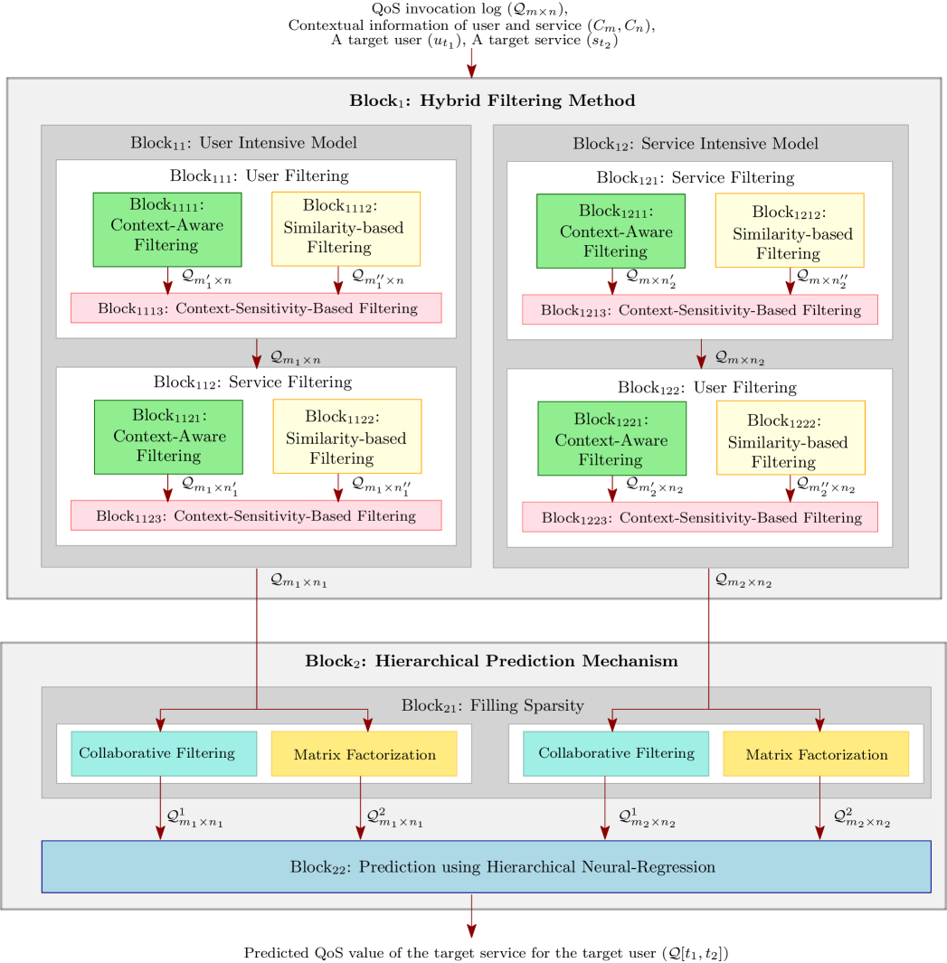
In this section, we discuss our solution framework to predict the target QoS value. Fig. 1 depicts the architecture of our framework (CAHPHF). The CAHPHF comprises two key steps, a hybrid filtering method followed by a hierarchical prediction mechanism, which are elaborated in the next two subsections.
3.1 Hybrid Filtering Method
This is the first phase of CAHPHF (referred to Block1 of Fig. 1). Given a target user and a target service, in this phase, we filter the set of users and the services considering different perspectives and principles.
We first consider two different aspects of filtering:
-
•
User-intensive filtering: In this case, we first filter the set of users and by leveraging refined user information, we filter the set of services.
-
•
Service-intensive filtering: In this case, we first filter the set of services. We further filter the set of users utilizing the filtered service information.
While filtering the users/services, we use two different principles:
-
•
Filtering based on contextual information of the users or services;
-
•
Filtering based on similarity information in terms of the historical QoS record.
Once we obtain the filtered users/services from the above two steps, we aggregate them by analyzing the context-sensitivity of the users/services to generate the final set of similar users/services, which is the output of the hybrid filtering.
We now illustrate each of the techniques mentioned above. We begin with discussing different filtering principles. We then elaborate on the inclusion of each of these approaches in our user-intensive and service-intensive filtering methods.
3.1.1 Context-Aware Filtering
As mentioned earlier in Section 2.1, we use the location information of the users/services as the contextual information in this paper. More specifically, we use latitude and longitude to refer to the location. Before discussing the details of context-aware filtering, we first define the contextual distance between two users/services. Here, we use the Haversine distance [28] function to refer to the contextual distance.
Definition 3.1.
[Haversine Distance ]: Given the location of two users/services and , the Haversine distance is computed as:
| (1) |
where ; either or . is the radius of the earth ( km) and represents inverse sine function.
Given a set of users/services and a target user/service, we compute a set of users/services similar to the target user/service in terms of contextual distance. Algorithm 1 presents the formal algorithm for computing the contextually similar users/services.
The main idea of Algorithm 1 is to generate a cluster containing all the users/services similar to the target user/service in terms of contextual distance. A tunable threshold parameter is chosen to filter the set of users (or services) to obtain the set of contextually similar users (or services ). If the distance between two users and (or two services and ) is less than , we add (or ) to (or ). We start with the target user (or service) and add it to (or ). Once a new user (or service ) is added to (or ), we follow the same procedure for (or ) as well. The algorithm terminates when there is no new user/service to be added. It may be noted that once the algorithm terminates, (or ) contains the set of users (or services) similar to the target user (or service), either directly or transitively. Here, we consider the transitive similarity, as this is required in the hierarchical prediction module to fill up the sparse matrix. We now consider a lemma with its proof as below.
Lemma 1.
, , where is the set of users similar to in terms of contextual distance.
Proof.
Consider . To prove , we need to show , and , . Now consider a user . This implies is either directly or transitively similar to in terms of contextual distance. Again, , and Haversine distance is commutative (i.e., ) imply is similar to (i.e., is similar to and is similar to , thereby is similar to ). This in turn implies that , .
Now consider a user . This implies is either directly or transitively similar to in terms of contextual distance according to Algorithm 1. is also similar to , since, . From the transitive property of Algorithm 1 and the commutative property of Haversine distance, we can conclude is also similar to (i.e., is similar to and is similar to , thereby, is similar to ). This implies, , .
, implies . Again, , implies . Both of them together imply . Hence, the above lemma is true. ∎
The same lemma is applicable for context-aware service filtering too, i.e., , , where is the set of services similar to in terms of contextual distance.
3.1.2 Similarity-based Filtering
The objective of this module is to obtain a set of users/services correlated to the target user/service in terms of their past QoS invocation histories. In this paper, we use cosine similarity function [29] to compute the correlation between two users/services as defined below.
Definition 3.2.
Algorithm 2 demonstrates the formal algorithm for generating the set of users/services correlated to the target user/service. Algorithm 2 is similar to Algorithm 1. The only difference is that instead of using Haversine distance function, cosine similarity measure is employed here. Similar to Algorithm 1, here also we use an external threshold parameter (or ) to filter the set of users/services. Like context-aware filtering (referred to Lemma 1), the similarity-based filtering also has the same characteristics as stated by Lemma 2.
Lemma 2.
, , where is the set of users correlated to in terms of cosine similarity.
It may be noted that the cosine similarity measure is also commutative. Therefore, using similar proof for Lemma 1, we can prove Lemma 2 as well. The same lemma is also applicable for similarity-based service filtering.
3.1.3 Context-Sensitivity-based Filtering
The goal of this module is to aggregate the results obtained by both context-aware filtering and similarity-based filtering modules by analyzing the context-sensitivity. Once we have a set of contextually similar users (or services ) and a set of correlated users (or services ) in terms of their past QoS records, the next objective is to aggregate them. The aggregation is performed on the basis of the similarity between these two sets. If the set of common users (or services) between and (or, and ) is more than a given threshold (or, ), this implies the QoS invocation pattern of the target user (or service) is context sensitive. In this case, we proceed with the intersection set. Otherwise, we proceed with set of correlated users/services. We now mathematically define, the filtering based on context-sensitivity as below.
| (4) |
| (5) |
We now prove the following lemma for filtering based on context-sensitivity, as follows.
Lemma 3.
, , where is the set of users similar to based on context-sensitivity.
Proof.
Similar to the above two filtering techniques, Lemma 3 is also valid for service filtering based on context-sensitivity.
We now discuss the user-intensive and service-intensive filterings in the next two subsections involving the filtering modules (i.e., context-aware, similarity-based, context-sensitivity-based) discussed above.
3.1.4 User-Intensive Filtering
Given a target service and a target user, in this step (referred to Block11 of Fig. 1), we first compute a set of users similar to the target user. Once we obtain the set of similar users, employing this information, we generate a set of services similar to the target service. Since in this filtering, we are leveraging the relevant user information to compute the set of similar services, this filtering is referred to user-intensive. We now demonstrate this approach in details.
As discussed earlier, the user-intensive filtering module comprises of two basic blocks: (a) Block111: user filtering block and (b) Block112: service filtering block (referred to Fig. 1). The main purpose of the user filtering block is to filter the set of users. Given a target user , the context-aware filtering and the similarity-based filtering are performed independently on the set of users, as discussed in Sections 3.1.1 and 3.1.2, to generate a set of contextually similar users and the set of correlated users , respectively. Once both the filterings are done, on the basis of context-sensitivity, and are aggregated to obtain the final set of similar users . Using the information of , the service filtering is performed similarly. Given a target service , context-aware filtering and similarity-based filtering are performed first on the set of services to generate a set of contextually similar services and the set of correlated services , respectively. Finally, on the basis of context-sensitivity, is generated from and . Algorithm 3 presents the formal algorithm for user-intensive filtering.
3.1.5 Service-Intensive Filtering
Given a target service and a target user, here (referred to Block12 of Fig. 1), initially, we compute a set of services similar to the target service. We then leverage related service information to obtain a set of users similar to the target user. Since in this filtering, we are utilizing relevant service information to compute the set of similar users, this filtering is termed as service-intensive. Algorithm 4 presents the formal algorithm for service-intensive filtering. Algorithm 4 is similar to Algorithm 3, where the only difference is in the sequence of the user and service-intensive filterings. The set of services, in this case, is filtered before the set of users.
Once we have the set of filtered users and services, we employ this information to predict the target QoS value. In the next section, we discuss our prediction mechanism.
3.2 Hierarchical Prediction Mechanism
This is the second phase of our framework (referred to Block2 of Fig. 1). The main focus of this module is to predict the target QoS value. We employ a hierarchical neural network-based regression model to predict the QoS value. It may be noted that the filtered QoS invocation log, which is used by the neural regression module to predict the QoS value, is mostly a sparse matrix. Therefore, in the hierarchical prediction module, our first task is to fill up the absent QoS values in the sparse matrix before feeding it to the hierarchical neural network.
3.2.1 Filling Sparsity
The goal of this module is to fill up the sparse invocation log matrix. In this paper, we employ collaborative filtering [2] and matrix factorization [30] to fill up the sparse matrix. We now briefly discuss these two approaches below.
3.2.1.1 Collaborative Filtering (CF): Collaborative filtering is one of the main approaches for QoS prediction. We first discuss the collaborative filtering method to fill up the filtered QoS invocation log matrix () obtained after user-intensive filtering. For every , we perform collaborative filtering. It may be noted that we do not need to filter the set of users/services anymore, since we have already performed filtering on the set of users and services in the hybrid filtering module. Moreover, it is clear from Lemma 3, if we wish to filter the set of users/services again using our hybrid filtering module, the number of users/services will not reduce any further. Therefore, in collaborative filtering, we only need to predict the QoS value, which is done using the following two steps: (a) average QoS computation and (b) calculation of deviation. In the average QoS calculation, we take the weighted column average corresponding to service , where the cosine similarity measures between and every other user in are used as the weights. Equation 6 shows the average QoS calculation for , as denoted by .
| (6) |
After having the average QoS value, we compute the deviation for accurate prediction. Here, we compute the deviation of the predicted value obtained by Equation 6 from the actual value across all services in and invoked by . The weighted average of the deviation, considering the cosine similarity measures between and every other service in as the weights, is adjusted to to obtain the predicted value of , as denoted by . Equation 7 shows the computation for deviation.
| (7) |
Finally, after employing the collaborative filtering to fill up every zero entry of , we have the modified QoS invocation log , as defined below:
| (8) |
The collaborative filtering to fill up obtained after service-intensive filtering is exactly same as in user-intensive case. For every , the collaborative filtering is performed. Equations 9 and 10 show the computations of average QoS value and deviation for each zero entry in , respectively.
| (9) |
| (10) |
Finally, after applying collaborative filtering on every zero entry of , we have the modified QoS invocation log , as defined below:
| (11) |
3.2.1.2 Matrix Factorization (MaF): Here, we employed the classical matrix factorization method [31] to generate modified QoS invocation logs and by filling up and , respectively.
It may be noted that after filling and , we now have 4 filled up matrices , , , and , which are used to predict the target QoS value using hierarchical neural regression. In the next part, we discuss the hierarchical neural regression.
3.2.2 Prediction using Hierarchical Neural Regression
This is the final phase of our framework, where we employ hierarchical neural network-based regression to predict the QoS value (referred to Fig. 2). The hierarchical neural regression module comprises of 2 key blocks: (a) Block222: Level-1 neural regression block (NRL-1), and (b) Block223: aggregator block (referred to Fig. 2). In addition to these two blocks, the hierarchical neural regression module contains another block, called controller (Block221), which mainly controls the aggregator block with the help of NRL-1. In NRL-1, we have 4 neural networks which are used to predict the target QoS values from , , , and , respectively. The aggregator block, then, aggregates the 4 QoS values obtained from NRL-1 with intending to increase the QoS prediction accuracy. In the aggregator module, we have 2 blocks, a Level-2 neural regression (NRL-2) block and a mean absolute error (MAE)-based aggregation (MAE-Ag) block. We invoke one of these two blocks, which is decided by the controller block on the basis of certain criteria as discussed latter in this section. We now describe each of the blocks of hierarchical neural regression module in details. We begin with describing Block222.
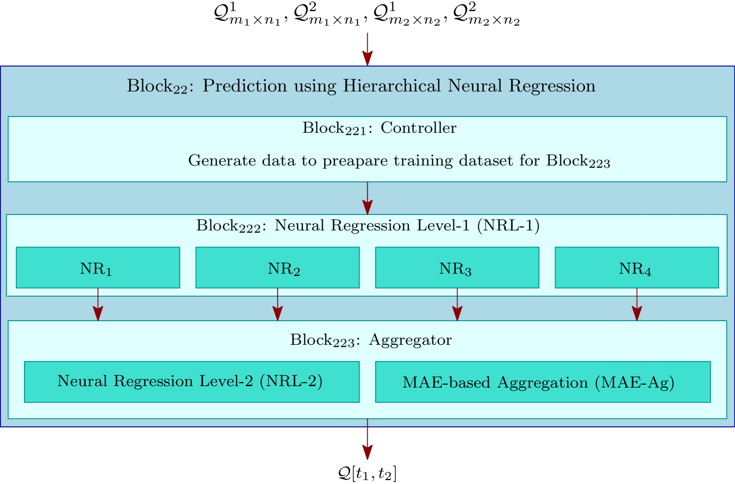
3.2.2.1 Neural Regression Level-1 (NRL-1): This is one of the major components of the hierarchical neural regression (referred to Block222 of Fig. 2). The module consists of 4 neural regression blocks NR1, NR2, NR3, and NR4. The goal of these 4 blocks is to predict the target QoS value from 4 QoS invocation log matrices obtained from Block21 of Fig. 1. Before going to the further details of NRL-1, we first describe the basic architecture of neural regression.
• Neural Regression (NR): In this paper, we employ a neural network-based regression module to predict the target QoS value. At the top of the NR module, a linear regression [32] layer is used to predict the missing QoS value. The objective of the linear regression is to generate a linear curve as defined: , where is a vector on the training dataset and . The set is the set of parameters required to be optimized to predict the QoS value accurately on the test dataset. It may be noted that represents the bias. To learn the value of each , a cost function is used, which is defined as: , where is the target value for the input vector and be the training dataset. To obtain the value of each , needs to be minimized, which actually represents the mean squared error (MSE). Here, we employ a feed-forward neural network with backpropagation [33] to obtain the values of . To optimize the cost function of the neural network, we use stochastic gradient descent (SGD) with momentum [33].
We now demonstrate the input-output of each of the 4 NR blocks below. Given a target user , a target service , a set of users , a set of services and a QoS invocation log matrix , the training-testing setup of each NR block is discussed below.
-
•
Training Data: For each user , the QoS invocation record vector from containing the QoS values for each service in is used as a training data. In other word, each row, except the one corresponding to , of is used as a training data of the neural regression.
-
•
Input Vector: For each training data, the QoS invocation record vector containing the QoS value of each service is used as the input vector for neural regression.
-
•
The Target Value: For each training data corresponding user , the QoS value of , i.e., is used as the target value of the neural regression.
-
•
Test Input Vector: For the user , the QoS invocation record vector corresponding to each service is used as the test input vector of the neural regression.
-
•
Test Output: Finally, the test output is the value of to be predicted.
It may be noted that NR1 and NR2 work on and , respectively corresponding to the user set and service set , while NR3 and NR4 work on and , respectively corresponding to the user set and service set . Consider and are the 4 outputs predicted by the 4 NR modules of Block222.
3.2.2.2 Controller Module: This is the first component (referred to Block221 of Fig. 2) of the hierarchical neural regression module. The objective of this module is to decide which component of the aggregator module to be executed and accordingly, either prepare the training dataset for NRL-2 or generate a dataset for MAE-Ag. The function of the controller is formally presented in Algorithm 5.
Given 4 QoS invocation log matrices and generated by Block21, the controller module first check if it is feasible to generate the dataset to train NRL-2. The essential idea behind NRL-2 is to compare the predicted values generated by the 4 NR blocks of NRL-1 with the actual QoS value. The comparison is possible only if the 4 NR blocks of NRL-1 can predict some QoS values, which are already available to the hierarchical neural regression module. The objective of the controller module is to choose a few entries from to be predicted by the 4 NR blocks of NRL-1 and to be compared the predicted values with the actual QoS value by NRL-2. Therefore, to train the NRL-2, sufficient entries are required in . A given threshold is used to check whether has sufficient entries to train NRL-2. If has sufficient entries to train NRL-2, the controller chooses a random number of entries from and execute 4 NR blocks of NRL-1 to obtain the predicted values. Once the predicted values from the NRL-1 are available, the controller module activates NRL-2 to obtain a more accurate predicted value. However, if does not have sufficient entries to train the NRL-2, the controller activates the MAE-Ag. In this case, to compute the MAE value of each NR block of NRL-1, the controller chooses random entries from each of and and executes the 4 NR blocks to obtain their MAE values. Finally, the controller activates MAE-Ag. The details of both the blocks of Block223 are discussed below.
3.2.2.3 Aggregator Module: This is the second major component of the hierarchical neural regression module (referred to Block223 of Fig. 2). The objective of this module is to generate a single predicted output by combining the 4 predicted values and obtained from the previous level while minimizing the prediction error. The aggregator module comprises of two components: (a) a Level-2 neural regression module (NRL-2) and (b) a MAE-based aggregation module (MAE-Ag). We now explain each of these two modules in details.
3.2.2.3.1 Neural Regression Level-2 (NRL-2): The objective of this module is to increase the prediction accuracy while aggregating the 4 predicted values obtained from NRL-1. Given a training dataset , and the 4 predicted values and obtained from Block222 as input, the training-testing setup of NRL-2 is discussed below:
-
•
Training Data: Each tuple , generated by Algorithm 5, is used as a training data.
-
•
Input Vector: The input vector contains the first 4 elements of .
-
•
The Target Value: The last element of is used as the target value.
-
•
Test Vector: The tuple is used as the test vector.
-
•
Test Output: The test output is the value of , which is to be predicted by Level-2 neural regression.
3.2.2.3.2 MAE-based Aggregation (MAE-Ag): The objective of this block is to compute the minimum MAE value among the 4 MAE values obtained from the 4 NR blocks of NRL-1 and accordingly chooses the NR block (say, MinNR block) generating the minimum MAE among the MAE values generated by all 4 NR blocks. Finally, MAE-Ag outputs the predicted value obtained by MinNR block, which is the final output of our framework. Algorithm 6 formally presents the MAE-Ag block.
In the following section, we provide rigorous experimental studies to justify the necessity of each block of our framework.
4 Experimental Results
In this section, we present the experimental results with analysis. We implemented our proposed framework in MATLAB R2019b. All experiments were executed on the MATLAB Online111https://matlab.mathworks.com server.
4.1 DataSets
(a) WS-DREAM-1: The first dataset contains 5825 services and 339 users. The location of each user and service is also provided in the dataset. The dataset comprises 2 QoS parameters: response time (RT) and throughput (TP). For each QoS parameter, the QoS invocation log with dimension is also given. We used both the QoS parameters to validate our approach.
(b) WS-DREAM-2: The second dataset contains 4500 services, 142 users, and 64 time slices. However, this dataset does not contain any contextual information. Similar to WS-DREAM-1, this dataset also comprises 2 QoS parameters: response time and throughput. For each QoS parameter, the QoS invocation log is also provided. For each time slice, we extracted the user-service matrix with dimension . We performed the experiment on 64 different matrices and recorded the average QoS prediction accuracy.
For experimental analysis, we divided each dataset into training, validation and testing sets. The size of the training dataset to be indicates entries of our QoS invocation log were randomly made as 0. The remaining entries are subdivided into validation and testing set into ratio.
We randomly chose 200 instances from the testing dataset for performance analysis. Each experiment was performed in 5 episodes for a given training dataset to find the prediction accuracy. Finally, the average result was calculated and reported in this paper.
4.2 Comparison Metric
We used the following two metrics to analyze our experimental results.
Definition 4.1.
[Mean Absolute Error (MAE)]: MAE is the arithmetic mean of the absolute difference between the predicted QoS value and the actual QoS value of a service invoked by a user over the testing dataset.
| (12) |
where is the actual QoS value, is the predicted QoS value, and is the testing dataset.
Definition 4.2.
[Improvement ]: Given two MAE values obtained by two methods and , the improvement of with respect to is defined as:
| (13) |
where and are the MAE values obtained by methods and , respectively.
4.3 Comparison Methods
We compare CAHPHF with a set of state-of-the-art methods followed by some intermediate methods to justify the performance of CAHPHF.
4.3.1 State-of-the-Art Methods
We compared the performance of CAHPHF with the following state-of-the-art approaches.
(i) UPCC [12]: This method exercised a user-based collaborative filtering approach for QoS prediction, where only the set of users similar to the target users were generated before applying the prediction strategy.
(ii) IPCC [13]: In this method, service-based collaborative filtering was applied for QoS prediction. The main idea in this work was to obtain a set of services similar to the target services first, followed by applying a prediction strategy.
(iii) WSRec [10]: This method combined both the strategies as demonstrated in UPCC and IPCC.
(iv) NRCF [9]: This method used normal recovery collaborative filtering to improve prediction accuracy.
(v) RACF [11]: This method also used collaborative filtering approach. Here, a ratio-based similarity metric was considered to compute the similarity, and the result was calculated by the similar users or similar services.
(vi) RECF [2]: A reinforced collaborative filtering approach was used in this work to predict the QoS value. This method integrated both user-based and service-based similarity information into a singleton collaborative filtering.
(vii) MF [20]: An extended matrix factorization-based approach was adopted in this work for prediction.
(viii) HDOP [34]: This method used multi-linear-algebra-based concepts of tensor for QoS value prediction. Tensor decomposition and reconstruction optimization algorithms were used to predict the QoS value.
(ix) TA [30]: This approach integrated time series ARIMA and GARCH models to predict the QoS value.
(x) NMF [35]: This approach proposed a non-negative matrix factorization method.
(xi) PMF [36]: This paper proposed a probabilistic matrix factorization method.
(xii) NIMF [15]: This approach proposed a user collaboration followed by a neighborhood-integrated matrix factorization for personalized QoS value prediction.
(xiii) CNR [25]: This method considered both user-intensive and service-intensive filtering in the filtering stage, and finally aggregated the output using the intersection between the set of users and services obtained from two different filtering methods. For prediction, this approach used neural regression to estimate the QoS value.
4.3.2 Intermediate Methods
We compared the performance of CAHPHF with the following intermediate methods, which is actually the ablation study of our system.
(i) User-intensive Matrix Factorization (UMF): In this approach, context-sensitive user-intensive filtering is performed first. Finally, matrix factorization is used on the filtered QoS invocation log matrix to predict the target QoS value.
(ii) Service-intensive Matrix Factorization (SMF): This approach is similar to UMF. The only difference is here, instead of applying the user-intensive filtering, the service-intensive filtering is adopted. In SMF, the context-sensitive service-intensive filtering is performed first, followed by a matrix factorization method to predict the QoS value.
(iii) User-intensive Collaborative Filtering (UCF): Here, the context-sensitive user-intensive filtering is performed first. Finally, collaborative filtering is used on the filtered QoS invocation log matrix to predict the target QoS value.
(iv) Service-intensive Collaborative Filtering (SCF): Here, the context-sensitive service-intensive filtering is performed first. Collaborative filtering is then employed to predict the desired QoS value.
(v) User-intensive Neural Regression (UNR): Similar to the UMF and UCF, in this approach, the context-sensitive user-intensive filtering is performed at the initial phase. However, unlike other methods, here, neural network-based regression is used on the filtered QoS invocation log matrix to predict the target QoS value.
(vi) Service-intensive Neural Regression (SNR): This approach is similar to UNR. The only difference is, in the filtering stage of this approach, the context-sensitive service-intensive filtering is performed.
(vii) User-intensive Matrix factorization with Neural Regression (UMNR): This approach is similar to UNR. However, in this approach, before applying neural network-based regression to predict the QoS value, matrix factorization is used to fill up the sparse matrix.
(viii) Service-intensive Matrix factorization with Neural Regression (SMNR): This approach is similar to SNR. However, like UMNR, in this approach, before applying neural network-based regression to predict the QoS value, matrix factorization is used to fill up the sparse matrix.
(ix) User-intensive Collaborative Neural Regression (UCNR): Unlike UMNR, here, before applying neural network-based regression to predict the QoS value, collaborative filtering is used to fill up the sparse matrix.
(x) Service-intensive Collaborative Neural Regression (SCNR): Unlike SMNR, here, before applying neural network-based regression to predict the QoS value, collaborative filtering is used to fill up the sparse matrix like UCNR.
(xi) CAHPHF Without NRL-1 (CAHPHFWoNN): This method is identical to the CAHPHF method except for one segment. In CAHPHFWoNN, instead of using NRL-1, collaborative filtering and matrix factorization are used to generate the training and testing dataset for NRL-2.
(xii) CAHPHF with minimum MAE (CAHPHF-MAE): This method is also similar to the CAHPHF method except for one portion. In CAHPHF-MAE, instead of using NRL-2, here, MAE-based aggregation method is used in of Fig. 2 to reduce error.
(xiii) User-intensive Collaborative Neural Regression Without Contextual Filtering (UCNRWoCF): This method is similar to the UCNR without contextual filtering.
(xiv) Service-intensive Collaborative Neural Regression Without Contextual Filtering (SCNRWoCF): This method is similar to the SCNR without contextual filtering.
(xv) User-intensive Matrix factorization with Neural Regression Without Contextual Filtering (UMNRWoCF): This method is similar to the UMNR without contextual filtering.
(xvi) Service-intensive Matrix factorization with Neural Regression Without Contextual Filtering (SMNRWoCF): This method is similar to the SMNR without contextual filtering.
(xvii) CAHPHF Without Contextual Filtering (CAHPHFWoCF): This method is similar to the CAHPHF without contextual filtering.
| QoS | MAE | (CAHPHF, CNR) | |||||||||
| UPCC | IPCC | WSRec | MF | NRCF | RACF | RECF | CNR | CAHPHF | |||
| RT | 10% | 0.6063 | 0.7 | 0.6394 | 0.5103 | 0.5312 | 0.4937 | 0.4332 | 0.2597 | 0.059 | 77.28% |
| 20% | 0.5379 | 0.5351 | 0.5024 | 0.4981 | 0.4607 | 0.4208 | 0.3946 | 0.1711 | 0.0419 | 75.51% | |
| 30% | 0.5084 | 0.4783 | 0.4571 | 0.4632 | 0.4296 | 0.3997 | 0.3789 | 0.0968 | 0.0399 | 58.78% | |
| \hlineB2.5 QoS | UPCC | IPCC | WSRec | NMF | PMF | NIMF | CAHPHF | (CAHPHF, NIMF) | |||
| TP | 5% | 26.123 | 29.265 | 25.8755 | 25.752 | 19.9034 | 17.9297 | 7.907 | 55.90% | ||
| 10% | 21.2695 | 27.3993 | 19.9754 | 17.8411 | 16.1755 | 16.0542 | 5.98 | 62.75% | |||
| 20% | 17.5546 | 25.0273 | 16.0762 | 15.2516 | 14.6694 | 13.7099 | 4.189 | 69.45% | |||
| : Size of Training Data | |||||||||||
4.4 Configuration of CAHPHF
In this subsection, we discuss the configuration used for CAHPHF method. We set the tunable parameters empirically from our validation dataset.
• Configuration of Hybrid Filtering: Here, a set of threshold parameters, more precisely 12 threshold parameters, is required. All these threshold parameters are data-driven.
The hybrid filtering comprises of 3 different filtering techniques. For context-aware filtering, the threshold values were chosen as:
| (14) |
| (15) |
where , are the contextual information of and respectively.
For similarity-based filtering, the threshold parameters were chosen as follows.
| (16) |
| (17) |
where the median was computed across for user filtering and for service filtering. As a matter of fact, the median of the similarity values can be 0, since the cosine similarity value varies from 0 to 1. Therefore, Equations 16 and 17 are different from Equations 14 and 15.
For context-sensitivity-based filtering, we used half of the cardinality value of the set of users or services obtained after similarity-based filtering.
| (18) |
| (19) |
• Configuration of NRL-1: Here, 4 neural networks are used. In our experiment, each neural network consisted of 2 hidden layers comprising of 256 and 128 neurons respectively. We used the following hyper-parameters for each neural network. The learning rate was set to 0.01 with momentum 0.9. The training was performed up to 50 epochs or up to a minimum gradient of .
• Configuration of NRL-2: Only 1 neural network is used in NRL-2 for which we used the following configuration. The network comprised of only 1 hidden layer with 2 neurons. Among the hyper-parameters, the learning rate was set to 0.01 with momentum 0.9. The training was performed up to 1000 epochs or up to a minimum gradient of . The cardinality of the training dataset to train NRL-2 was taken as 200.
We provide a rigorous analysis of parameter tuning latter in this section.
4.5 Experimental Analysis
In Table II, we present the performance of our CAHPHF in terms of MAE considering the response time (RT) and throughput (TP) individually as the QoS parameter over WS-DREAM-1. Along with the performance study of CAHPHF, Table II shows a comparative study with the major state-of-the-art approaches.
In WS-DREAM-2, the contextual information of the users and services are not present. Therefore, instead of CAHPHF, Table III shows the comparison between CAHPHFWoCF and the major state-of-the-art approaches considering RT and TP individually over WS-DREAM-2.
| QoS | MAE | |||||
| MF | TA | HDOP | CAHPHFWoCF | |||
| RT | 10% | 0.4987 | 0.6013 | 0.3076 | 0.1187 | 61.41% |
| 20% | 0.4495 | 0.5994 | 0.2276 | 0.0758 | 66.70% | |
| 50% | 0.4013 | 0.4877 | 0.1237 | 0.0326 | 73.65% | |
| \hlineB2.5 TP | 10% | 16.3214 | 17.2365 | 13.2578 | 4.897 | 63.06% |
| 20% | 14.1478 | 15.0994 | 10.1276 | 4.101 | 59.51% | |
| 50% | 14.9013 | 14.9870 | 10.0037 | 3.561 | 64.40% | |
| : Size of Training Data, : (CAHPHFWoCF, HDOP) | ||||||
From the experimental results, we have the following observations:
-
(i)
As evident from Tables II and III, our methods performed the best as compared to the major state-of-the-art approaches for both the QoS parameters RT and TP. The last columns of the above tables show the improvement of our method over the second-best method of Tables II and III. On average our framework achieves 65.7% improvement as compared to the second-best state-of-the-art method of Tables II and III.
-
(ii)
It is observed from Fig.s 3 (a) and (b) that MAE value decreases and thus, the prediction accuracy improves with the increase in the size of the training dataset.
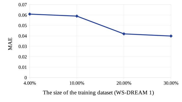
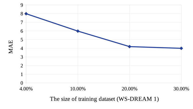
(a) (b)
From now on we show the experimental results on response time of WS-DREAM-1, since for the rest of the datasets, similar trends are observed.
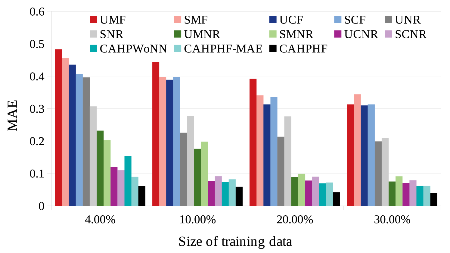
Fig. 4 shows the comparison between CAHPHF and the intermediate methods (referred to Section 4.3.2). As evident from Fig. 4, CAHPHF produced the best results compared to all the intermediate methods. The significance of each block of CAHPHF is discussed below.
-
(i)
UNR and SNR are better than UMF, SMF, UCF, and SCF, which signifies the importance of the neural regression used in our framework.
-
(ii)
UMNR, SMNR, UCNR, and SCNR are better than UNR and SNR, which clearly establishes the requirement of our hierarchical prediction strategy, more specifically the need for filling up the sparse matrix.
-
(iii)
CAHPHF is better than UMNR, SMNR, UCNR, and SCNR, which signifies the requirement of the hierarchical neural regression (more specifically, Block223) module and as well as hybrid filtering.
-
(iv)
CAHPHF is also better than CAHPHFWoNN, which also signifies the requirement of the hierarchical neural regression (more specifically, Block222) module.
-
(v)
Finally, CAHPHF is better than CAHPHF-MAE, which clearly shows the importance of the Level-2 neural regression module.
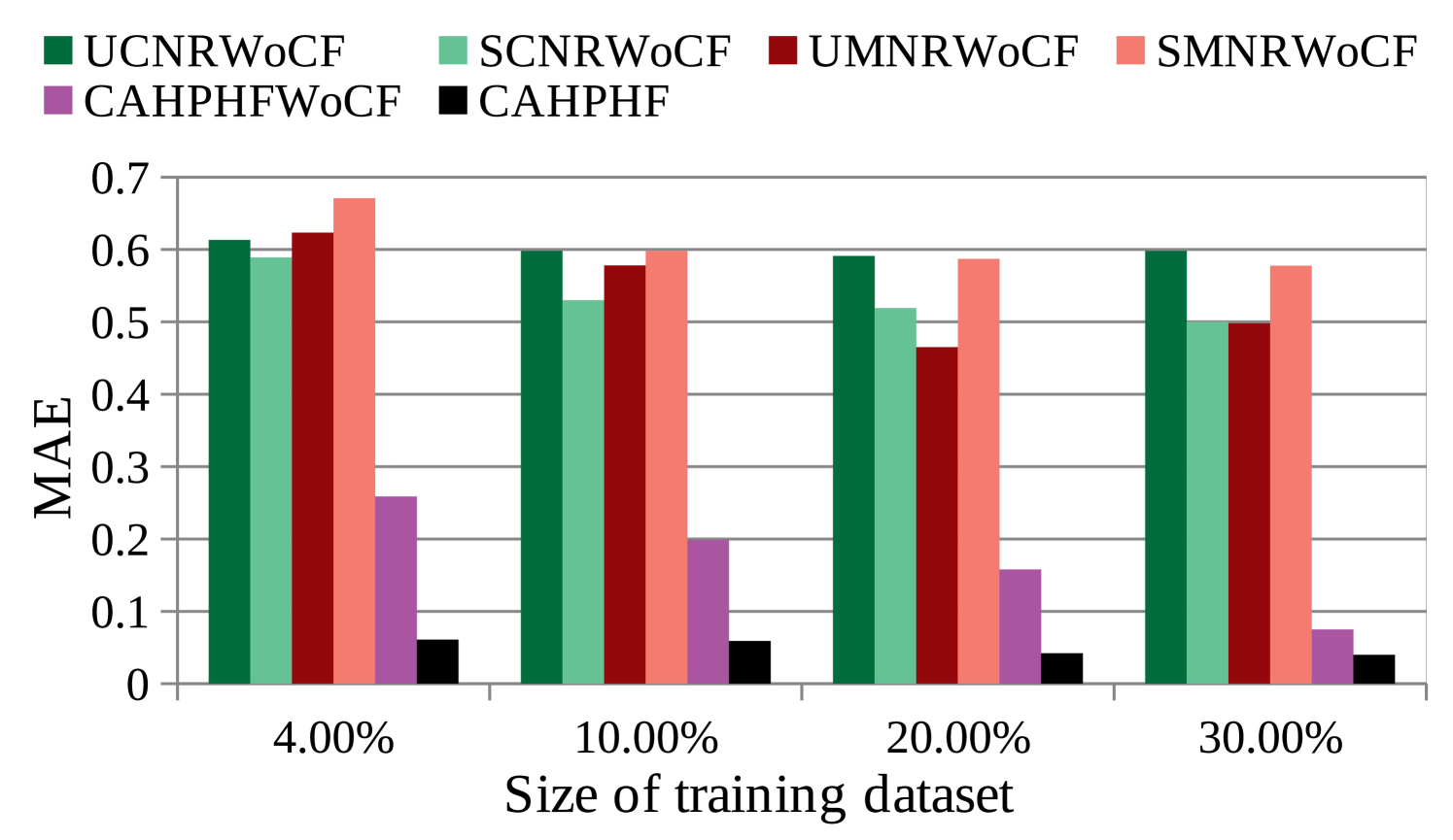
4.5.1 Context-Sensitivity Analysis
Fig. 5 shows the significance of context-sensitive filtering used in our approach. We compared our proposed method with the intermediate methods without context sensitive filtering (referred to Section 4.3.2). As evident from Fig. 5, CAHPHF outperformed the rest of the methods. Here, we have the following observations:
-
(i)
CAHPHFWoCF is better than SCNRWoCF, SMNRWoCF, UCNRWoCF, and UMNRWoCF, which implies the significance of our hybrid filtering module.
-
(ii)
As CAHPHF is better than CAHPHFWoCF, it implies that the context sensitivity analysis is quite impactful in our framework.
4.5.2 Impact of Tunable Parameters
In this subsection, we show the impact of tunable parameters on the prediction accuracy of CAHPHF. In this analysis, for each experiment, we varied one parameter at a time, while keeping the rest of the parameters as constant, same as discussed in Section 4.4. We begin with discussing the impact of the threshold parameter required in hybrid filtering module on the prediction accuracy.
4.5.2.1 Impact of Threshold Parameter: Before analyzing the impact of the threshold parameters on the prediction accuracy, we first discuss the tuning of these parameters. In this experiment, we chose a variable to tune the threshold parameters, as explained below.
(i) In context aware filtering, the set of users/services to be filtered was sorted in descending order based on their contextual distances from the target user/service. From the sorted list, the contextual distance (say, ) between the user/service and the target user/service was chosen as threshold (i.e., /), where be the set of users/services to be filtered. It may be noted, by varying , we obtained different values of /.
(ii) In similarity-based filtering, the set of users/services to be filtered was sorted in ascending order based on their cosine similarity values with the target user/service. From the sorted list, the cosine similarity value (say, ) of the user/service with the target user/service was chosen as the threshold (i.e., /), where is the set of users/services to be filtered. Finally, was chosen as the value of /, where is the maximum cosine similarity value across all users/services with the target user/service.
(iii) For context sensitive filtering, the threshold / was chosen as fraction of the cardinality of the set of users/services obtained after similarity-based filtering.
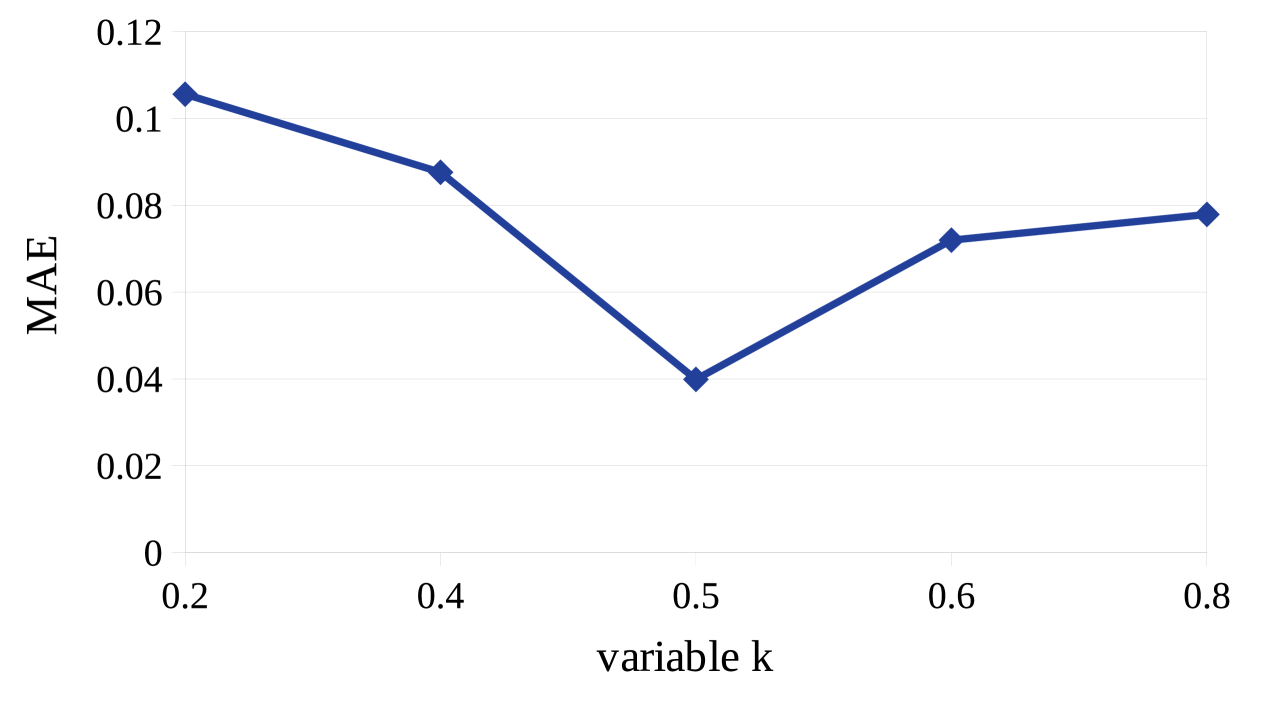
Fig. 6 shows the change in MAE with respect to . As evident from Fig. 6, for , the least MAE value was obtained, which we used in our experiment. It may be noted, as we increased the value of beyond 0.5, the MAE value reduced, because of the following fact. Due to a high value of , the values of the threshold parameters were also very high. Therefore, the filtered set of users/services contained only a few numbers of users/services, which was insufficient to train the neural network in the latter part of our framework. On the other hand, for lower values of the threshold parameters, the filtered set of users/services contained a large number of users/services, which in turn impeded the objective of the filtering. Consequently, MAE reduced with the decrease in the value of .
4.5.2.2 Impact of training data size of NRL-2: It may be observed, the size of the dataset to train NRL-2 (say, ) has an impact on the prediction accuracy. While Fig. 7(a) shows the change in MAE with increase in , Fig. 7(b) shows the computation time required by CAHPHF with the change in . It may be noted further, the -axis of Fig.s 7(a), (b) represent the training data size of CAHPHF, whereas, the legends of the figures represent the size of . As observed from Fig.s 7(a), (b), the MAE value decreased with the increase in while compromising the computation time. Clearly, we have a trade-off between computation time and prediction accuracy. Furthermore, we observe from Fig.s 7(a), (b) that even our worst performance (i.e., the MAE value obtained by CAHPHF when ) was better than the state-of-the-art approaches of Table II. Therefore, as per the permitted time limit, the size of is to be decided.
(a)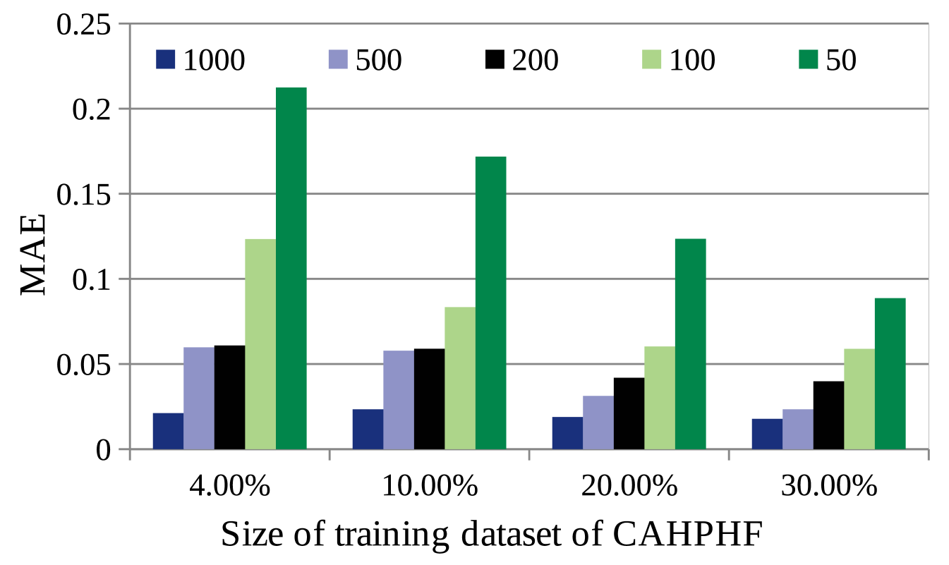 (b)
(b)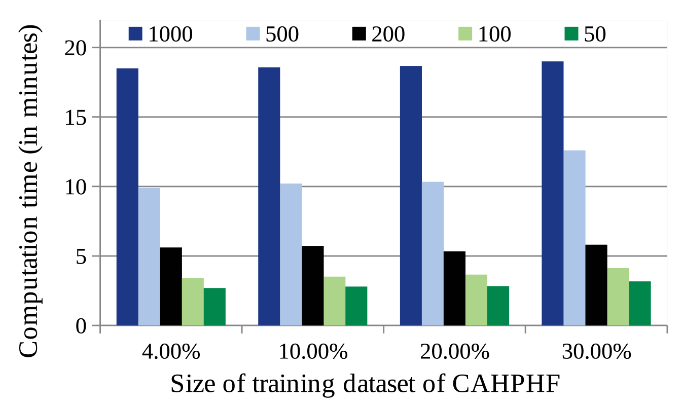
(a)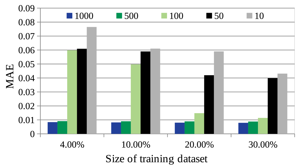 (b)
(b)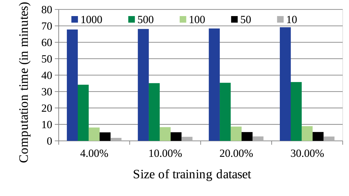
(a)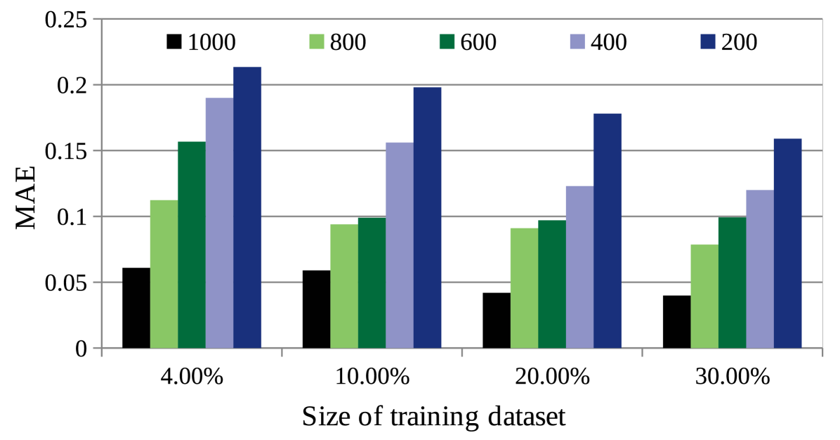 (b)
(b)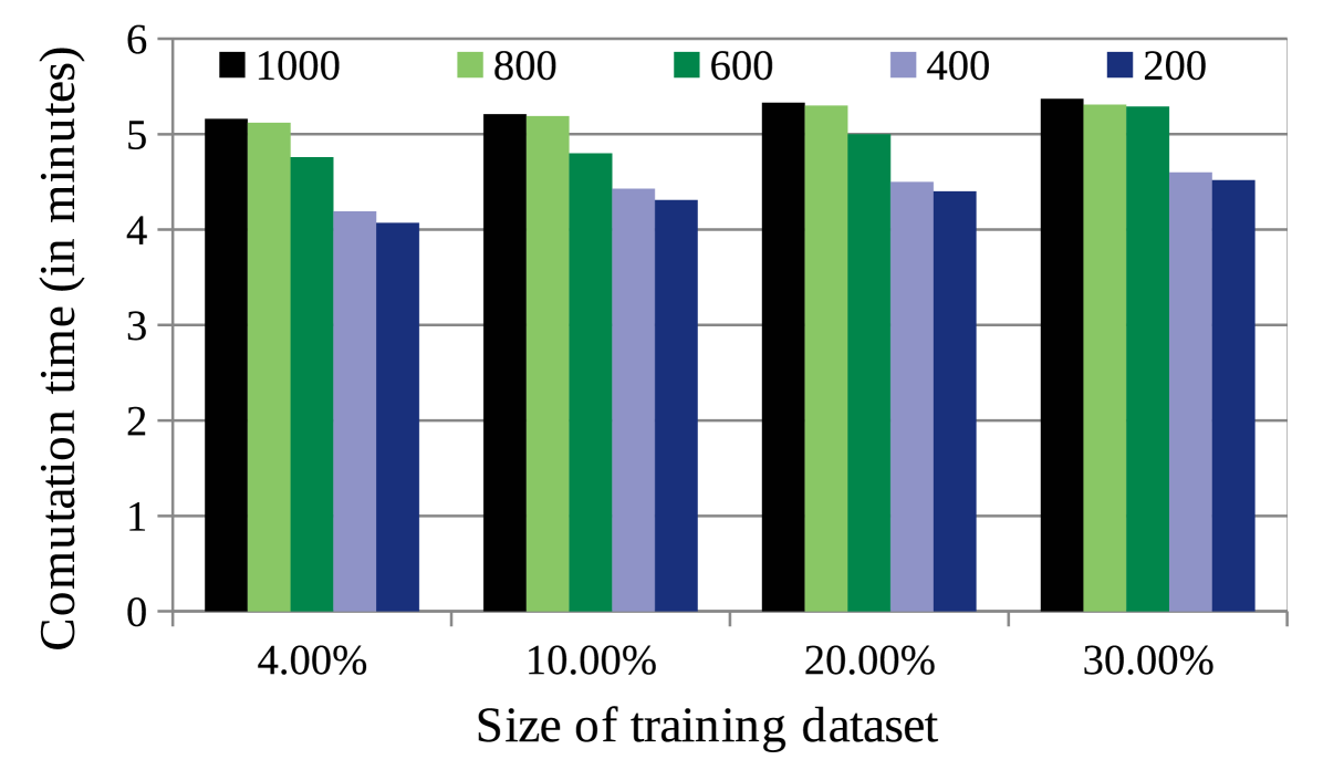
4.5.2.3 Impact of Hyper-parameters of NR: Here, we mainly discuss about 3 hyper-parameters of the neural networks: (a) the number of epochs in each NR of NRL-1, (b) the number of epochs in NRL-2, and (c) the number of hidden layers of each NR in NRL-1. The other tunable parameters of the neural networks such as number of neurons in each hidden layer, the learning rate, momentum, minimal gradient value, etc. were also empirically decided.
Fig. 8(a) shows the change in MAE value with the increase in the number of epochs of each NR of NRL-1, while Fig. 8(b) shows the corresponding time to predict the QoS value by CAHPHF. It is observed from Fig.s 8(a), (b), the more time we spent to train the neural network, better was the solution quality. This statement is true at-least up to a certain number of epochs. Therefore, here also, we observed the time-quality trade-off. However, along with achieving a high prediction accuracy, our framework should be robust. Therefore, considering the permitted time-limit, we need to choose the number of epochs of each NR of NRL-1. It may be noted, here also, in the worst case (i.e., the number of epochs of each NR of NRL-1 = 10), the MAE value obtained by CAHPHF was better than the state-of-the-art approaches of Table II.
Similar to the Fig.s 8(a), (b), we show the time-quality trade-off with respect to the number of epochs of NRL-2 in Fig.s 9(a), (b). The previous analysis is also valid here.
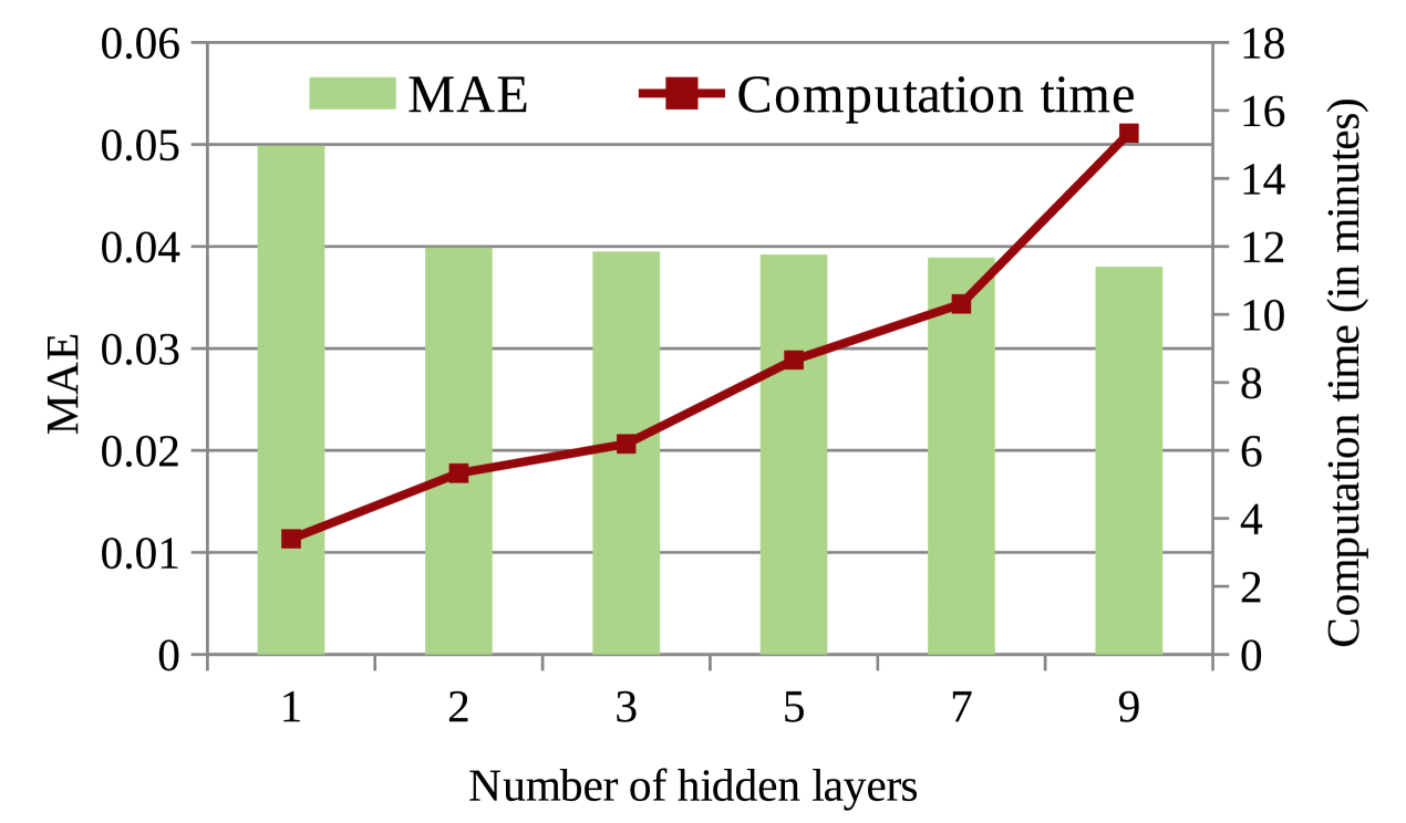
Fig. 10 shows the change in MAE value with respect to the number of hidden layers of each NR in NRL-1. The primary and secondary vertical axes of Fig. 10 represent MAE and computation time, respectively. As observed from this figure, the MAE value decreases with an increase in the number of hidden layers of the neural networks. However, with the increase in the number of hidden layers of the neural networks, computation time to generate the solution also increases. Therefore, here also, the number of hidden layers are chosen as per allowed time-limit.
In summary, our proposed CAHPHF, on the one hand, outperformed the state-of-the-art methods in terms of prediction accuracy, on the other hand, it generated the solution in a reasonable time limit.
5 Related Work
The QoS parameter plays a crucial role in various operations of the services life cycle, e.g., service selection [37, 38, 39], service composition [40, 41, 42], service recommendation [2, 3]. The major limitation of most of these studies is that the service QoS values are assumed to be known. However, the QoS value of service often changes across various factors, such as user [2, 11], time [3], location [43, 18, 15], etc. Therefore, QoS prediction is an integral part of a service life cycle.
The QoS prediction has been studied broadly in the literature [44, 45, 46, 47, 48]. The collaborative filtering is one of the major techniques to address the QoS prediction problem. The collaborative filtering can be of two different types: model-based and memory-based. The memory-based collaborative filtering [9, 11, 3, 7, 8, 2] is further classified into two categories: user-based and service-based. In user-based collaborative filtering [6, 15, 12], the similar users are taken into account to predict the QoS value, while in service-based collaborative filtering [13], the similar services are considered for QoS prediction. In this context, various similarity measures have been used to obtain the set of similar users or services, e.g., Pearson Correlation Coefficient (PCC) [8], cosine similarity measure [25], etc. Some enhanced similarity measures [3, 7] have also been introduced to improve prediction accuracy. However, the stand alone user-based or service-based collaborative filtering may not be very effective concerning prediction accuracy, since it does not consider similar services (or, users) in a user-based (or, service-based) approach, and therefore, the prediction accuracy is not satisfactory. To achieve a higher prediction accuracy, both the techniques are combined further to predict the QoS values [3, 7, 8, 2]. However, the prediction accuracy of memory-based collaborative filtering approaches fall significantly for the sparse matrix.
| State-of- | Methods | QoS | Dimension | ||||
| the-Art | CF | MaF | Reg | RT | TP | Time | Location |
| [8] | U + S | ✓ | ✓ | ||||
| [2, 11, 9] | U + S | ✓ | |||||
| [7] | U + S | ✓ | ✓ | ✓ | ✓ | ||
| [43] | U + S | ✓ | ✓ | ✓ | |||
| [6] | U | ✓ | ✓ | ✓ | ✓ | ||
| [3] | U + S | ✓ | ✓ | ✓ | |||
| [15] | U | ✓ | ✓ | ✓ | ✓ | ||
| [19] | ✓ | ✓ | ✓ | ||||
| [24] | ✓ | ✓ | ✓ | ||||
| [18] | U + S | ✓ | ✓ | ✓ | |||
| [17] | U + S | ✓ | ✓ | ✓ | ✓ | ✓ | ✓ |
| [25] | U + S | ✓ | ✓ | ✓ | |||
| [23] | ✓ | ✓ | ✓ | ✓ | |||
| [45] | U + S | ✓ | ✓ | ✓ | |||
| [12] | U | ✓ | ✓ | ||||
| [13] | S | ✓ | ✓ | ||||
| [20] | U + S | ✓ | ✓ | ||||
| [34] | ✓ | ✓ | ✓ | ✓ | |||
| [14] | ✓ | ✓ | ✓ | ✓ | ✓ | ||
| [49] | ✓ | ✓ | ✓ | ||||
| U: user-based; S: service-based; Reg: regression | |||||||
To resolve the problem with the sparse matrix and to improve the accuracy, a model-based collaborative approach is implemented. In the model-based collaborative filtering, a predefined model is adapted according to the given dataset. One such method is matrix factorization [18, 19, 15, 17], which is employed for solving the sparsity problem in memory-based collaborative filtering technique. The matrix factorization involves decomposing the QoS invocation log matrix into a low-rank approximation that makes further predictions. However, in the traditional matrix factorization method, the predicted value lacks accuracy. Therefore, regularisation terms is included in the loss function of matrix factorization [18, 19, 15, 20] to avoid overfitting [33] in learning process and to improve the prediction accuracy. To elevate this accuracy further, the collaborative filtering method is integrated with the matrix factorization, where the collaborative filtering utilizes the local information, and the matrix factorization uses global information for value prediction [18, 15, 17]. Sometimes, the matrix factorization is combined with the recurrent neural network [17] to obtain better results. In [17], a personalized LSTM (Long Short-Term Memory)-based matrix factorization is proposed to capture the temporal dependencies of both users and services to timely update prediction model with data. Some other approaches [18, 15] in the literature have used a few other information (e.g., geographic location for neighborhood similarity calculation) in addition to the matrix factorization for improving accuracy level. On a similar note, for multi-dimensional QoS prediction problem, a tensor decomposition and reconstruction method [34] has been used for QoS values prediction. Although, matrix factorization can handle the sparsity problem, most of the times it suffers from loss of information [19].
Another popular model-based technique is regression [24]. In [25, 23, 50], the neural regression has been proposed to obtain better accuracy. Some neural network-based models exist in the literature to predict QoS value, e.g., back-propagation neural network [24], feed forward neural network [25], neural network with radial basis function [23], etc. Predicting QoS values only on the basis of neural regression may not provide satisfactory outcome. Therefore, improvisation of the regression method has been introduced. For example, in [50], a clustering of similar users on the basis of location along with the neural regression for QoS prediction has been proposed. In [25], a neural regression with filtering has been proposed, where a set of similar users and services are generated first, and then neural regression is employed to predict the QoS value. However, in [25], an ad-hoc approach is used to handle the sparsity problem. The authors in [45] has proposed QoS prediction with auto-encoder, where there is a model entitled that combines both model-based and memory-based approaches for QoS value prediction. However, the predicted QoS value is yet to reach the satisfactory level. Table IV provides a briefing on the reported works that addressed the prediction problem.
In contrast to the above approaches, our current paper addresses the QoS prediction problem by taking advantage of both the memory-based and model-based techniques. The proposed framework is of two-folds, hybrid filtering, followed by hierarchical prediction. Our filtering technique, on the one side, combines both user-based and service-based approaches, while on the other side, it is a coalition of user-intensive and service-intensive models to capture the priority of users and services. Moreover, to achieve better accuracy, our filtering technique leverages the location information of users and services. Furthermore, we apply a clustering technique to obtain a set of similar context-sensitive users and services. Our hierarchical prediction mechanism takes advantage of the model-based approach. To deal with the sparsity problem, we use collaborative filtering along with the matrix factorization to fill up the matrix. We then employ a hierarchical neural regression to predict the QoS value. On the one hand, our hierarchical neural regression fixes the QoS prediction problem. On the other hand, it helps in reducing the error in prediction. Our extensive experimental analysis also justifies the necessity of each segment of our framework.
6 Conclusion
In this paper, we propose a hierarchical QoS prediction mechanism with hybrid filtering by leveraging the contextual information of users and services. Our approach takes benefit of the memory-based strategies by consolidating filtering and the model-based strategies by combining hierarchical prediction. Additionally, we handle the sparsity issue by filling up the absent values in the matrix using collaborative filtering and matrix factorization. Finally, we increase the prediction accuracy by aggregating the predicted values obtained by user-intensive and service-intensive modules using hierarchical neural regression. We performed extensive experiments on publicly available WS-DREAM benchmark datasets. The experimental results show that the proposed CAHPHF framework is better than the state-of-the-art approaches in terms of prediction accuracy, while justifying the requirement of each module of our framework. In the future, we will endeavor to work on a time-variant QoS prediction mechanism.
References
- [1] H. Wu et al., “A Hybrid Approach to Service Recommendation based on Network Representation Learning,” IEEE Access, vol. 7, pp. 60 242–60 254, 2019.
- [2] G. Zou et al., “QoS-Aware Web Service Recommendation with Reinforced Collaborative Filtering,” in ICSOC, 2018, pp. 430–445.
- [3] J. Li et al., “Temporal Influences-Aware Collaborative Filtering for QoS-based Service Recommendation,” in IEEE SCC, 2017, pp. 471–474.
- [4] R. Ramacher and L. Mönch, “Cost-Minimizing Service Selection in the Presence of End-to-End QoS Constraints and Complex Charging Models,” in IEEE SCC, 2012, pp. 154–161.
- [5] S. Chattopadhyay, A. Banerjee, and T. Mukherjee, “A Framework for Top Service Subscription Recommendations for Service Assemblers,” in IEEE SCC, 2016, pp. 332–339.
- [6] C. Wu et al., “Time-Aware and Sparsity-Tolerant QoS Prediction based on Collaborative Filtering,” in IEEE ICWS, 2016, pp. 637–640.
- [7] C. Yu and L. Huang, “A Web Service QoS Prediction Approach based on Time- and Location-Aware Collaborative Filtering,” SOCA, vol. 10, no. 2, pp. 135–149, 2016.
- [8] Z. Zhou et al., “QoS-Aware Web Service Recommendation Using Collaborative Filtering with PGraph,” in IEEE ICWS, 2015, pp. 392–399.
- [9] H. Sun et al., “Personalized Web Service Recommendation via Normal Recovery Collaborative Filtering,” IEEE TSC, vol. 6, no. 4, pp. 573–579, 2013.
- [10] Z. Zheng et al., “QoS-Aware Web Service Recommendation by Collaborative Filtering,” IEEE TSC, vol. 4, no. 2, pp. 140–152, 2011.
- [11] X. Wu et al., “Collaborative Filtering Service Recommendation based on A Novel Similarity Computation Method,” IEEE TSC, vol. 10, no. 3, pp. 352–365, 2017.
- [12] J. S. Breese et al., “Empirical Analysis of Predictive Algorithms for Collaborative Filtering,” in Uncertainty in artificial intelligence. Morgan Kaufmann Publishers Inc., 1998, pp. 43–52.
- [13] B. M. Sarwar et al., “Item-based Collaborative Filtering Recommendation Algorithms,” WWW, vol. 1, pp. 285–295, 2001.
- [14] T. Chen et al., “Personalized Web Service Recommendation based on QoS Prediction and Hierarchical Tensor Decomposition,” IEEE Access, vol. 7, pp. 62 221–62 230, 2019.
- [15] Z. Zheng et al., “Collaborative Web Service QoS Prediction via Neighborhood Integrated Matrix Factorization,” IEEE TSC, vol. 6, no. 3, pp. 289–299, 2013.
- [16] Y. Xu, J. Yin, and W. Lo, “A Unified Framework of QoS-based Web Service Recommendation with Neighborhood-Extended Matrix Factorization,” in IEEE SOCA 2013, 2013, pp. 198–205.
- [17] R. Xiong, J. Wang, Z. Li, B. Li, and P. C. K. Hung, “Personalized LSTM Based Matrix Factorization for Online QoS Prediction,” in IEEE ICWS, 2018, pp. 34–41.
- [18] K. Qi et al., “Personalized QoS Prediction via Matrix Factorization Integrated with Neighborhood Information,” in IEEE SCC, 2015, pp. 186–193.
- [19] X. Luo et al., “Predicting Web Service QoS via Matrix-Factorization-based Collaborative Filtering under Non-Negativity Constraint,” in WOCC 2014, 2014, pp. 1–6.
- [20] W. Lo et al., “An Extended Matrix Factorization Approach for QoS Prediction in Service Selection,” in IEEE SCC. IEEE, 2012, pp. 162–169.
- [21] T. Alam et al., “An Effective Recursive Technique for Multi-Class Classification and Regression for Imbalanced Data,” IEEE Access, vol. 7, pp. 127 615–127 630, 2019.
- [22] D. Bissing et al., “A Hybrid Regression Model for Day-Ahead Energy Price Forecasting,” IEEE Access, vol. 7, pp. 36 833–36 842, 2019.
- [23] P. Zhang et al., “A Combinational QoS-Prediction Approach based on RBF Neural Network,” in IEEE SCC, 2016, pp. 577–584.
- [24] H. Chen, “Back-Propagation Neural Network for QoS Prediction in Industrial Internets,” in CollaborateCom, 2016, pp. 577–582.
- [25] S. Chattopadhyay and A. Banerjee, “QoS Value Prediction Using a Combination of Filtering Method and Neural Network Regression,” in ICSOC 2019, 2019, pp. 135–150.
- [26] Z. Zheng et al., “Investigating QoS of Real-World Web Services,” IEEE TSC, vol. 7, no. 1, pp. 32–39, 2014.
- [27] Y. Zhang, Z. Zheng, and M. R. Lyu, “WSPred: A Time-Aware Personalized QoS Prediction Framework for Web Services,” in IEEE ISSRE, 2011, pp. 210–219.
- [28] S. Wang et al., “QoS Prediction for Service Recommendations in Mobile Edge Computing,” Journal of Parallel and Distributed Computing, vol. 127, pp. 134–144, 2019.
- [29] J. Zhu, P. He, Z. Zheng, and M. R. Lyu, “A Privacy-Preserving QoS Prediction Framework for Web Service Recommendation,” in IEEE ICWS. IEEE, 2015, pp. 241–248.
- [30] A. Amin, A. Colman, and L. Grunske, “An Approach to Forecasting QoS Attributes of Web Services based on ARIMA and GARCH Models,” in IEEE ICWS, 2012, pp. 74–81.
- [31] Å. Björck, Numerical Methods in Matrix Computations. Springer, 2015, vol. 59.
- [32] S. Lathuilière et al., “A Comprehensive Analysis of Deep Regression,” IEEE TPAMI, 2019.
- [33] I. Goodfellow, Y. Bengio, and A. Courville, Deep learning. MIT press, 2016.
- [34] S. Wang et al., “Multi-Dimensional QoS Prediction for Service Recommendations,” IEEE TSC, 2016.
- [35] D. D. Lee and H. S. Seung, “Learning the Parts of Objects by Non-Negative Matrix Factorization,” Nature, vol. 401, no. 6755, p. 788, 1999.
- [36] A. Mnih and R. R. Salakhutdinov, “Probabilistic Matrix Factorization,” in Advances in neural information processing systems, 2008, pp. 1257–1264.
- [37] H. Alayed et al., “Enhancement of Ant Colony Optimization for QoS-Aware Web Service Selection,” IEEE Access, vol. 7, pp. 97 041–97 051, 2019.
- [38] F. Dahan, H. Mathkour, and M. Arafah, “Two-Step Artificial Bee Colony Algorithm Enhancement for QoS-Aware Web Service Selection Problem,” IEEE Access, vol. 7, pp. 21 787–21 794, 2019.
- [39] D. Li et al., “Service Selection With QoS Correlations in Distributed Service-based Systems,” IEEE Access, vol. 7, pp. 88 718–88 732, 2019.
- [40] N. Chen, N. Cardozo, and S. Clarke, “Goal-Driven Service Composition in Mobile and Pervasive Computing,” IEEE TSC, vol. 11, no. 1, pp. 49–62, 2018.
- [41] M. Amini and F. Osanloo, “Purpose-based Privacy Preserving Access Control for Secure Service Provision and Composition,” IEEE TSC, vol. 12, no. 4, pp. 604–620, 2019.
- [42] S. Chattopadhyay, A. Banerjee, and N. Banerjee, “A Fast and Scalable Mechanism for Web Service Composition,” TWEB, vol. 11, no. 4, pp. 26:1–26:36, 2017.
- [43] K. Chen et al., “Trust-Aware and Location-based Collaborative Filtering for Web Service QoS Prediction,” in IEEE COMPSAC, 2017, pp. 143–148.
- [44] X. Luo et al., “An Effective Scheme for QoS Estimation via Alternating Direction Method-based Matrix Factorization,” IEEE TSC, vol. 12, no. 4, pp. 503–518, 2019.
- [45] Y. Yin et al., “QoS Prediction for Mobile Edge Service Recommendation with Auto-Encoder,” IEEE Access, vol. 7, pp. 62 312–62 324, 2019.
- [46] W. Xiong et al., “A Learning Approach to QoS Prediction via Multi-Dimensional Context,” in IEEE ICWS, 2017, pp. 164–171.
- [47] K. Lee, J. Park, and J. Baik, “Location-based Web Service QoS Prediction via Preference Propagation for Improving Cold Start Problem,” in IEEE ICWS, 2015, pp. 177–184.
- [48] C. Wu et al., “QoS Prediction of Web Services based on Two-Phase K-Means Clustering,” in IEEE ICWS, 2015, pp. 161–168.
- [49] L. Guo et al., “Personalized QoS Prediction for Service Recommendation With a Service-Oriented Tensor Model,” IEEE Access, vol. 7, pp. 55 721–55 731, 2019.
- [50] Y. Shi et al., “A New QoS Prediction Approach based on User Clustering and Regression Algorithms,” in IEEE ICWS, 2011, pp. 726–727.
![[Uncaptioned image]](https://cdn.awesomepapers.org/papers/2734ca29-93e6-4d2f-848d-559bcdaa27d4/rrcg.png) |
Ranjana Roy Chowdhury received her B.Tech in Computer Science and Engineering (CSE) from Assam University, Silchar, India, in 2017. Currently, she is pursuing her M.Tech in CSE from Indian Institute of Information Technology Guwahati, India. Her research interests include Services Computing, Machine Learning-related subjects. |
![[Uncaptioned image]](https://cdn.awesomepapers.org/papers/2734ca29-93e6-4d2f-848d-559bcdaa27d4/scgr.png) |
Soumi Chattopadhyay (S’14, M’19) received her Ph.D. from Indian Statistical Institute, Kolkata in 2019. Currently, she is an Assistant Professor in Indian Institute of Information Technology Guwahati, India. Her research interests include Distributed and Services Computing, Artificial Intelligence, Formal Languages, Logic and Reasoning. |
![[Uncaptioned image]](https://cdn.awesomepapers.org/papers/2734ca29-93e6-4d2f-848d-559bcdaa27d4/cag.jpg) |
Chandranath Adak (S’13, M’20) received his Ph.D. in Analytics from University of Technology Sydney, Australia in 2019. Currently, he is an Assistant Professor at Centre for Data Science, JIS Institute of Advanced Studies and Research, India. His research interests include Image Processing, Pattern Recognition, Document Image Analysis, and Machine Learning-related subjects. |