Caloric curves of self-gravitating fermions in general relativity
Abstract
We study the nature of phase transitions between gaseous and condensed states in the self-gravitating Fermi gas at nonzero temperature in general relativity. The condensed states can represent compact objects such as white dwarfs, neutron stars, or dark matter fermion balls. The caloric curves depend on two parameters: the system size and the particle number . When , where is the Oppenheimer-Volkoff limit, there exists an equilibrium state for any value of the temperature and of the energy as in the nonrelativistic case [P.H. Chavanis, Int. J. Mod. Phys. B 20, 3113 (2006)]. Gravitational collapse is prevented by quantum mechanics (Pauli’s exclusion principle). When , there is no equilibrium state below a critical energy and below a critical temperature. In that case, the system is expected to collapse towards a black hole. We plot the caloric curves of the general relativistic Fermi gas, study the different types of phase transitions that occur in the system, and determine the phase diagram in the plane. The nonrelativistic results are recovered for and with fixed. The classical results are recovered for and with fixed. We discuss the commutation of the limits and . We study the relativistic corrections to the nonrelativistic caloric curves and the quantum corrections to the classical caloric curves. We highlight a situation of physical interest where a gaseous Fermi gas, by cooling, first undergoes a phase transition towards a compact object (white dwarf, neutron star, dark matter fermion ball), then collapses into a black hole. This situation occurs in the microcanonical ensemble when . We also relate the phase transitions from a gaseous state to a core-halo state in the microcanonical ensemble to the onset of red-giant structure and to the supernova phenomenon.
pacs:
95.30.Sf, 95.35.+d, 04.40.Dg, 67.85.Lm, 05.70.-a, 05.70.FhI Introduction
The study of phase transitions is an important problem in physics. Some examples include solid-liquid-gas phase transitions, superconducting and superfluid transitions, Bose-Einstein condensation, liquid-glass phase transition in polymers, liquid crystal phases, Kosterlitz-Thouless transition etc. Self-gravitating systems also undergo phase transitions but they are special due to the unshielded long-range attractive nature of the interaction paddy . This leads to unusual phenomena such as negative specific heats, ensembles inequivalence, long-lived metastable states, and gravitational collapse. A strict equilibrium state can exist only if the system is confined within a box, otherwise it has the tendency to evaporate (this is already the case for an ordinary gas). On the other hand, in order to define a condensed phase we need to introduce a short-range repulsion between the particles that opposes itself to the gravitational attraction.111Without small-scale regularization, there is no equilibrium state (global entropy maximum) in a strict sense antonov . There can exist, however, metastable gaseous states (local entropy maxima) that are insensistive to the small-scale regularization antonov ; lbw . These metastable states have a very long lifetime, scaling as , where is the number of particles in the system lifetime . In practice this lifetime is much larger than the age of the Universe, making the metastable states fully relevant in astrophysics ijmpb . In this paper, we consider the case of self-gravitating fermions where an effective short-range repulsion is due to quantum mechanics (Pauli’s exclusion principle). The object of this paper is to present a complete description of phase transitions in the self-gravitating Fermi gas in general relativity. This study can have applications in relation to the formation of compact objects such as white dwarfs, neutron stars, dark matter stars, black holes etc. On the other hand, the phase transition from a gaseous state to a condensed state may be related to the onset of red-giant structure and to the supernova phenomenon. We first start by reviewing the literature on the subject. We focus our review on papers that study phase transitions in the box-confined self-gravitating Fermi gas at nonzero temperature.222The case of completely degenerate self-gravitating fermions at and the case of classical (nondegenerate) self-gravitating systems are considered in our companion papers paper1 ; paper2 where a detailed review of the literature is made. We do not review the immensely vast literature related to self-gravitating fermions as models of white dwarfs, neutron stars, and dark matter halos. For a connection to this literature, we refer to chandrabook ; shapiroteukolsky ; btv ; vss ; rar ; clm1 ; clm2 ; urbano ; rsu and references therein. For a connection to the general literature on the statistical mechanics of self-gravitating systems and systems with long-range interactions we refer to the introduction of sd and to the reviews paddy ; houches ; katzrevue ; ijmpb ; cdr ; campabook .
The statistical mechanics of nonrelativistic self-gravitating fermions at nonzero temperature enclosed within a box of radius was first studied by Hertel & Thirring (1971) htf . They worked in the canonical ensemble and rigorously proved that the mean field approximation (or effective field approximation) and the Thomas-Fermi (TF) approximation (which amounts to neglecting the quantum potential) become exact in a suitable thermodynamic limit where , , , , and (the scaling was first obtained by Lévy-Leblond (1969) levyleblond for the ground state).333This is also equivalent to the usual thermodynamic limit where , , , and with (see Appendix A). This leads to the temperature-dependent TF equation.444It can be obtained by combining the fundamental equation of hydrostatic equilibrium with the Fermi-Dirac equation of state or, equivalently, by substituting the Fermi-Dirac density into the Poisson equation; see, e.g., Hertel (1977) hseul . For that reason, the temperature-dependent TF equation is sometimes called the Fermi-Dirac-Poisson equation. The existence of the TF limit for the thermodynamic functions of self-gravitating fermions was proven by Hertel et al. (1972) hnt for the microcanonical and canonical ensembles and by Messer (1979) messer for the grand canonical ensemble. The convergence of the quantum-statistically defined particle density towards the TF density was proven by Baumgartner (1976) baumgartner . He also showed that there are no correlations in the thermodynamic limit. Narnhofer and Sewell (1980) ns1 showed that when the equilibrium Gibbs distribution becomes a tensor product of density functions of an ideal Fermi gas which minimize the TF free energy functional. These density functions can be stable (global minima) or metastable (local minima). Finally, Narnhofer and Sewell (1982) ns2 showed that when a quantum system of self-gravitating fermions is described by the classical Vlasov equation bh .
Hertel & Thirring (1971) ht studied numerically phase transitions in the nonrelativistic self-gravitating Fermi gas in relation with the structure of neutron stars.555The possibility of phase transitions in the self-gravitating Fermi gas at nonzero temperature was suggested in the Appendix IV of Lynden-Bell and Wood (1969) lbw . They assumed that the gas is enclosed within a box and worked in the canonical ensemble. For a given number of particles , they showed that a canonical first order phase transition arising from a multiplicity of solutions in the TF equation appears if the radius of the box is larger than a certain value . This phase transition is characterized by a jump of energy (the energy , the first derivative of with respect to , becomes discontinuous) at a transition temperature determined by a Maxwell construction like in the theory of the van der Waals gas.666The phase transition arises because the TF equation has two stable solutions at the same temperature that minimize the TF free energy. A rigorous analytical proof for the existence of this phase transition was given by Messer (1981a,1981b) messerpt1 ; messerpt2 following numerical calculations by Hertel (1977) hseul . When there are multiple solutions in the TF equation, they argue that one must choose the one with the smallest value of free energy. This corresponds to a transition between a nearly homogeneous phase of medium mass density (gaseous phase) and a phase with a high density core surrounded by an atmosphere of low density (condensed phase) when the system cools down below . Hertel & Thirring (1971) ht explained that this phase transition replaces the region of negative specific heats in the microcanonical ensemble (or the piece of convex curvature in the entropy curve ) which is associated with unstable equilibrium states in the canonical ensemble. Therefore, the microcanonical and canonical ensembles are not equivalent hnt . The region of negative specific heat in the microcanonical ensemble is bridged by a phase transition in the canonical ensemble.777Canonical phase transitions, associated with negative specific heats, have also been found by Thirring (1970) thirring in a toy model of self-gravitating systems, by Aronson and Hansen (1972) ah for a self-gravitating hard spheres gas, by Carlitz (1972) carlitz for hadronic matter, and by Hawking (1976) hawking for black holes. Hertel & Thirring (1971) ht applied their crude model of neutron stars to a system of neutrons (the corresponding mass being of the order of the solar mass) initially contained in a sphere of radius . The critical radius is . For , the system undergoes a first order phase transition below a critical temperature , collapses, and forms a compact object (neutron star) containing almost all the mass. This compact object has approximately the same size, , as a completely degenerate Fermi gas at (equivalent, in their nonrelativistic model, to a polytrope of index ) but it is surrounded by a small isothermal atmosphere. This gravitational phase transition could account for the implosion of the core in the supernova phenomenon where the energy is carried quickly by neutrinos.888Thirring (1970) thirring , Hertel and Thirring (1971) ht and Messer (1981) messerpt2 mention the analogy between this phase transition and the formation of red giants and supernovae. However, this analogy may not be fully correct because the phase transition that they obtain just corresponds to an implosion. This is because they work in the canonical ensemble and consider relatively small systems while the phase transition leading to an implosion-explosion phenomenon, associated with a core-halo structure, occurs in the microcanonical ensemble for larger systems (see Ref. supernova and Sec. XIII). Lynden-Bell and Wood (1968) lbw , considering a classical self-gravitating gas in the microcanonical ensemble, find the emergence of a core-halo structure and relate it to the onset of red giants.
Gravitational phase transitions of fermionic matter were also studied by Bilic & Viollier (1997) bvn in a cosmological setting. They considered weakly interacting massive fermions of mass in the presence of a large radiation-density background fixing the temperature. They studied a halo of mass and radius . When the system cools down below a transition temperature , a condensed phase emerges consisting of quasidegenerate supermassive fermion stars of mass and radius . They argued that these compact dark objects could play an important role in structure formation in the early Universe. In particular, these fermion stars could explain, without resorting to the black hole hypothesis, some of the features observed around supermassive compact dark objects which are reported to exist at the centers of a number of galaxies including our own and quasistellar objects (QSOs). On a technical point of view, their study is analogous to the one carried out by Hertel & Thirring (1971) ht for neutron stars, i.e., they described the canonical first order phase transtion between a “gaseous” phase and a “condensed” phase that appears below a transition temperature when the size of the object is sufficiently large.
A detailed theoretical description of phase transitions in the nonrelativistic self-gravitating Fermi gas at nonzero temperature was given by Chavanis (2002) ijmpb (see also Refs. csmnras ; pt ; dark ; ispolatov ; rieutord ; ptd ).999In these papers, the statistical equilibrium state is obtained by maximizing the Fermi-Dirac entropy at fixed mass and energy in the microcanonical ensemble and by minimizing the Fermi-Dirac free energy at fixed mass in the canonical ensemble, where is obtained from a combinatorial analysis taking into account the Pauli exclusion principle. This leads to the TF (or Fermi-Dirac-Poisson) equation in a direct manner. The study of the self-gravitating Fermi gas has also applications in the statistical theory of violent relaxation developed by Lynden-Bell lb that also leads to a Fermi-Dirac-type distribution csmnras . He showed that the caloric curves depend on a single control parameter with ( is the spin multiplicity of the quantum states). For a fixed particle number , this paramerer can be seen as a measure of the size of the system since . Chavanis ijmpb studied in detail the nature of phase transitions in the nonrelativistic self-gravitating Fermi gas in both microcanonical and canonical ensembles. He showed that there exist two critical points (one in each ensemble) at which zeroth and first order phase transitions appear. The canonical critical point at which canonical phase transitions appear is equivalent to the one previously found by Hertel and Thirring (1971) ht . The microcanonical critical point at which microcanonical phase transitions appear was not found previously. For , one recovers the caloric curve of a nonrelativistic self-gravitating classical gas paddy . Chavanis ijmpb ; lifetime argued that first order phase transitions do not take place in practice, contrary to previous claims ht ; bvn , because of the very long lifetime of metastable states for systems with long-range interactions. Therefore, only zeroth order phase transitions take place at the spinodal points where the metastable branches disappear. Recently, this study of phase transitions was extended to the nonrelativistic fermionic King model clm1 ; clm2 . This model is more realistic as it avoids the need of an artificial box to confine the system.
Gravitational phase transitions of fermionic matter in general relativity were studied by Bilic and Viollier (1999) bvr .101010In that case, the suitable thermodynamic limit corresponds to where , , , and with bvr . This is also equivalent to the usual thermodynamic limit where , , , and with (see Appendix A). They showed that, at some critical temperature , weakly interacting massive fermionic matter with a total mass below the Oppenheimer-Volkoff (OV) limit ov undergoes a first order gravitational phase transition from a diffuse to a clustered state, i.e., a nearly completely degenerate fermion star. This is an extension of their previous paper bvr in the Newtonian approximation. This relativistic extension allowed them to consider situations where the mass of the system is close to the OV limit so that the fermion star is strongly relativistic. For fermions masses of to they argued that these fermions stars may well provide an alternative explanation for the supermassive compact dark objects that are observed at galactic centers. Indeed, a few Schwarzschild radii away from the object, there is little difference between a supermassive black hole and a fermion star of the same mass near the OV limit.111111Some difficulties with the “fermion ball” scenario to provide an alternative to supermassive black holes at the centers of the galaxies are pointed out in genzel . In their paper, they considered fermionic particles of mass for which , , and . They studied a system of fermions, corresponding to a rest mass which is slightly below the OV limit, in a sphere of size . The transition occurs at . This leads to a fermion star containing almost all the particles surrounded by a small atmosphere. If we approximate the fermion star by a Fermi gas at containing all the rest mass , we find a radius and a mass .
The study of Bilic and Viollier bvr is restricted to a unique value of and , with , leading to a canonical phase transition. The object of this paper is to perform a more general study of phase transitions in the self-gravitating Fermi gas in general relativity for arbitrary values of and . In particular, we would like to determine what happens when , or what happens for larger values of where a microcanonical phase transition is expected.
The paper is organized as follows. In Sec. II, we present the basic equations describing a general relativistic Fermi gas at statistical equilibrium in a box. In Sec. III, we expose general notions concerning the construction of the caloric curves and the description of phase transitions. In Sec. IV, we recall the results previously obtained in the nonrelativistic and classical limits. In Sec. V, we consider the case where the system undergoes a canonical phase transition from a gaseous phase to a condensed phase when . In Sec. VI, we consider the case where the system undergoes a canonical phase transition when and a microcanonical phase transition when (we find that and ). In Sec. VII, we consider the case of very large radii where extreme core-halo configurations with a high central density appear. They correspond to the solutions computed in btv ; rar ; clm2 in connection to the “fermion ball” scenario. However, following clm2 , we point out that these solutions are thermodynamically unstable (hence very unlikely). In Secs. VIII and IX, we consider the cases and where there is no phase transition. In Sec. X, we present the complete phase diagram of the general relativistic Fermi gas in the plane. In Sec. XI, we recover the nonrelativistic and classical results as particular limits of our general study and we discuss the commutation of the limits and . In Sec. XII, we study the relativistic corrections to the nonrelativistic caloric curves and the quantum corrections to the classical caloric curves. In Sec. XIII, we consider astrophysical applications of our results in relation to the formation of white dwarfs, neutron stars, dark matter fermion stars, and black holes. We also connect the phase transitions found in our study with the onset of the red-giant structure and with the supernova phenomenon.
II Basic equations of a general relativistic Fermi gas
In this section, we give the basic equations describing the structure of a general relativistic Fermi gas at nonzero temperature (see bvcqg ; bvr ; papiertheorique for their derivation). Using the normalized variables introduced in Appendix B, the local number density , the energy density , the pressure and the temperature are related to the gravitational potential by
| (1) |
| (2) |
| (3) |
| (4) |
where
| (5) |
is a quantity that is uniform throughout the system. These equations define the equation of state of a relativistic Fermi gas in parametric form.
The Tolman-Oppenheimer-Volkoff (TOV) equations, which correspond to the equations of hydrostatic equilibrium in general relativity, can be written as
| (6) |
| (7) |
where is the mass-energy within the sphere of radius . They have to be solved with the boundary conditions
| (8) |
We assume that the system is confined within a box of radius . The total mass of the gas and the total particle number are given by
| (9) |
| (10) |
The temperature at infinity is given by
| (11) |
where is the temperature of the system on the edge of the box. Using Eq. (4), we obtain
| (12) |
The entropy is given by
| (13) |
Finally, the free energy is given by
| (14) |
where is the binding energy.121212The binding energy is usually defined as . Here, for convenience, we define it with the opposite sign, i.e., . In the Newtonian limit, and reduces to the usual energy which is the sum of the kinetic and potential (gravitational) energies.
III Caloric curves and phase transitions
In order to study the phase transitions in the general relativistic Fermi gas we have to determine the caloric curves relating the temperature at infinity to the energy . These caloric curves depend on two parameters and . The manner to obtain these caloric curves is detailed in Appendix C. In order to make the connection with the nonrelativistic results ijmpb , we shall plot the caloric curves in terms of the dimensionless parameters (inverse temperature) and (minus energy) defined by
| (15) |
where and . In terms of our normalized variables, they reduce to
| (16) |
where and . We shall therefore plot the caloric curves as a function of and .
We recall that for systems with long-range interactions, such as self-gravitating systems, the statistical ensembles are not equivalent. In this paper, we shall consider the microcanonical and canonical ensembles separately.
In the microcanonical ensemble, the system is isolated so that its energy is conserved. It serves as a control parameter. A stable equilibrium state is a (local) maximum of entropy at fixed energy and particle number . A minimum, or a saddle point, of entropy is unstable. The global maximum of entropy corresponds to the most probable state (the one that is the most represented at the microscopic level). The microcanonical caloric curve gives the temperature at infinity as a function of the energy .
In the canonical ensemble, the system is in contact with a heat bath so that its temperature at infinity is fixed. It serves as a control parameter. A stable equilibrium state is a (local) minimum of free energy at fixed temperature and particle number . A maximum, or a saddle point, of free energy is unstable. The global minimum of free energy corresponds to the most probable state. The caloric curve gives the average energy as a function of the temperature at infinity .
The equilibrium states are the same in the microcanonical and canonical ensembles. This is because an extremum (first variations) of entropy at fixed energy and particle number coincides with an extremum of free energy at fixed particle number. However, their stability (second variations) may differ in the microcanonical and canonical ensembles. A configuration that is stable in the canonical ensemble is necessarily stable in the microcanoniocal ensemble but the converse is wrong. As a corollary we recall that the specific heat of stable equilibrium states is always positive in the canonical ensemble while it can be positive or negative in the microcanonical ensemble (for systems with long-range interactions).
The stability of the solutions can be determined by using the Poincaré turning point criterion poincare . We refer to the papers of Katz katzpoincare1 ; katzpoincare2 for a presentation and a generalization of this criterion, and for its application to the nonrelativistic classical self-gravitating gas. This method was applied to the nonrelativistic self-gravitating Fermi gas in ijmpb . We use the same method in the present paper.
In the discussion of the caloric curves, we shall only consider stable states. An equilibrium state that is a local, but not a global, extremum of the relevant thermodynamical potential (entropy in the microcanonial ensemble and free energy in the canonical ensemble) is said to be metastable. A global extremum of the thermodynamical potential is said to be fully stable. For systems with short-range interactions, metastable states have a short lifetime so that the caloric curve should contain only fully stable states. However, for systems with long-range interactions, the metastable states have a very long lifetime scaling as which is usually much longer than the age of the Universe. As a result, metastable states can be as much, or even more, relevant than fully stable states lifetime . The selection between a fully stable state or a metastable state depends on the initial condition and on a notion of basin of attraction. In this paper, we shall not distinguish between metastable and fully stable states. The physical caloric curve should contain all types of stable equilibrium states.131313The existence, or nonexistence, of fully stable states for self-gravitating fermions in general relativity is an interesting problem by itself but it will not be considered in the present paper (see the Remark at the end of Sec. V.3 showing that this problem is not trivial).
For real systems, that are not in a box, the natural evolution proceeds along the series of equilibria towards larger and larger density contrasts.141414The reason is that, for real systems (globular clusters, dark matter halos…) such as those described by the King model, the Boltzmann or Fermi-Dirac entropy (resp. the Boltzmann or Fermi-Dirac free energy) increases (resp. decreases) with the concentration parameter; see Fig. 5 of cohn and Fig. 46 of clm2 . Note that, surprisingly, for box-confined systems this is the opposite; see Fig 3 of pt . In general, this corresponds to lower and lower temperatures and energies.151515This is explicitly shown in Figs. 12 and 15 below. Note that this result is valid only for mid and low energies and temperatures. At very high energies and temperatures, where the system behaves as a self-gravitating radiation, the density contrast increases with the energy and the temperature (see Figs. 2 and 3 of paper2 ) implying that the natural evolution of the system is towards higher and higher energies and temperatures. This situation has been discussed in paper2 and will not be considered here. Therefore, in the discussion of the caloric curves, we shall describe the evolution of the system starting from high energies and high temperatures, and reducing the temperature and the energy until an instability takes place.
IV Particular limits
In this section, we briefly recall well-known results that correspond to particular limits of the general relativistic Fermi gas.
IV.1 The nonrelativistic classical limit
The thermodynamics of a nonrelativistic classical self-gravitating gas has been studied in detail in antonov ; lbw ; katzpoincare1 ; paddyapj ; aa . The caloric curve forms a spiral (see Fig. 1). In the microcanonical ensemble, there is no equilibrium state below a critical energy corresponding to . In that case, the system undergoes a gravothermal catastrophe (core collapse) leading to a binary star surrounded by a hot halo lbe ; inagaki ; cohn . In the canonical ensemble, there is no equilibrium state below a critical temperature , corresponding to . In that case, the system undergoes an isothermal collapse leading to a Dirac peak containing all the mass post .

IV.2 The nonrelativistic limit
The thermodynamics of the nonrelativistic self-gravitating Fermi gas has been studied in detail in ijmpb . It is shown that the caloric curves depend on a single control parameter (it should not be confused with the chemical potential):
| (17) |
It can be written as ijmpb :
| (18) |
or as
| (19) |
where (resp. ) is the radius (resp. mass) of a fermion star of mass (resp. radius ) at (see Appendix F). Introducing the normalized variables of Appendix B, this parameter becomes
| (20) |
Some caloric curves are represented in Fig. 2. They display a canonical critical point at and a microcanonical critical point at . When there is no phase transition. When the system displays zeroth and first order canonical phase transitions. When the system displays zeroth and first order canonical and microcanonical phase transitions. When we recover the caloric curve of the nonrelativistic classical self-gravitating gas (spiral) represented in Fig. 1. When there is a statistical equilibrium state for any accessible value of energy and temperature. The gravitational collapse of the nonrelativistic classical self-gravitating gas (gravothermal catastrophe in the microcanonical ensemble and isothermal collapse in the canonical ensemble) is prevented by quantum mechanics (Pauli’s exclusion principle).

For a given box radius, the nonrelativistic canonical phase transition appears when
| (21) |
If we consider the general relativistic problem, we must require , where is the OV limit, for the validity of the nonrelativistic treatment. Therefore, we will see the nonrelativistic canonical phase transition for provided that
| (22) |
In comparison . This argument just provides an order of magnitude of the radius above which a canonical phase transition appears for . By solving the general relativistic equations, we find that the exact value is (see Sec. X).
For a given box radius, the nonrelativistic microcanonical phase transition appears when
| (23) |
If we consider the general relativistic problem, using the same argument as before, we will see the nonrelativistic microcanonical phase transition for provided that
| (24) |
This argument just provides an order of magnitude of the radius above which a microcanonical phase transition appear for . By solving the general relativistic equations, we find that the exact value is (see Sec. X).
IV.3 The classical limit
The thermodynamics of a classical self-gravitating gas in general relativity has been studied in detail in Refs. roupas and paper2 . This corresponds to the nondegenerate limit of the general relativistic Fermi gas. It is shown that the caloric curves depend on a single control parameter
| (25) |
It can be written as
| (26) |
or as
| (27) |
where can be interpreted as a sort of Schwarzschild radius defined with the rest mass instead of the mass (reciprocally, is a sort of Schwarzschild rest mass of an object of radius ). Introducing the normalized variables of Appendix B this parameter becomes
| (28) |

Some caloric curves are represented in Fig. 3. When ( or ), we recover the caloric curve of the nonrelativistic classical self-gravitating gas (spiral) represented in Fig. 1. When the caloric curve has the form of a double spiral exhibiting a collapse at low energies and low temperatures (cold spiral) and at high energies and high temperatures (hot spiral).161616The hot spiral corresponds to an ultrarelativistic classical gas roupas which is similar to a form of radiation described by an equation of state sorkin ; aarelat1 ; aarelat2 (see paper2 for a detailed discussion). When the two spirals are amputed (truncated) and touch each other. When the two spirals disappear and the caloric curve makes a loop resembling to the symbol “”. As increases, the loop shrinks more and more and, when , it reduces to a point located at . When , no equilibrium state is possible.
For a given box radius, the spirals touch each other when
| (29) |
and they form a loop when
| (30) |
The caloric curve reduces to a point when
| (31) |
If we consider the truly quantum problem, we must require for the validity of the classical (nondegenerate) treatment. Therefore, we will see the double spiral and its evolution described previously for provided that
| (32) |
We note that is of the order of .
Remark: For a given box radius , coming back to dimensional variables, equilibrium states exist only when . Inversely, for a given number of particles , equilibrium states exist only when . The nonrelativistic limit corresponds to or . These results are valid in the classical limit. For small systems, quantum effects will come into play. If we argue that when , or equivalently when , we find that . This may justify the order of magnitude of this constant. Alternatively, we may just remark that is of the same order as .
IV.4 Summary
Before treating the general case, let us summarize the previous results.
Nonrelativistic classical limit. For a given box radius and particle number the system undergoes a catastrophic collapse towards a singularity at low temperatures in the canonical ensemble and at low energies in the microcanonical ensemble.
Nonrelativistic limit. For a given box radius there is no phase transition when , the system can undergo a canonical phase transition when , and the system can undergo a canonical and a microcanonical phase transition when . For a given particle number , there is no phase transition when , the system can undergo a canonical phase transition when , and the system can undergo a canonical and a microcanonical phase transition when . Here, and are the reciprocal of and . There is an equilibrium state at all temperatures in the canonical ensemble and at all accessible energies (where is the energy of the ground state) in the microcanonical ensemble.
Classical limit. For a given box radius , the caloric curve has the form of a double spiral when , the spirals touch each other when , the caloric curve makes a loop when , and there is no equilibrium state when . For a given particle number , the caloric curve has the form of a double spiral when , the spirals touch each other when , the caloric curve makes a loop when , and there is no equilibrium state when . Here, , and are the reciprocal of , and . The system undergoes a catastrophic collapse towards a singularity at both low and high temperatures in the canonical ensemble and at both low and high energies in the microcanonical ensemble.
V The case
In this section, we study the general relativistic Fermi gas in the case where only a canonical phase transition may occur (see Fig. 47 below). For illustration, we select . For this value of , the canonical phase transition occurs above .
V.1 The case
In Fig. 4 we have plotted the caloric curve for . Since , this caloric curve coincides with the one obtained in the nonrelativistic limit ijmpb except at very high energies and very high temperatures (see the Remark at the end of this section).171717As discussed in Sec. XI the nonrelativistic limit corresponds to and in such a way that is fixed (in more physical terms and with fixed).

The series of equilibria is monotonic. According to the Poincaré theory of linear series of equilibria, all the equilibrium states are stable. The statistical ensembles (microcanonical and canonical) are equivalent. The caloric curve presents the following features:
(i) There is no phase transition and no gravitational collapse.
(ii) The specific heat is always positive. The entropy versus energy curve (not represented) is concave.
The evolution of the system is the following. At high energies and high temperatures, the system is nondegenerate (Boltzmannian). As the energy and the temperature are reduced, the system becomes more and more centrally condensed. At intermediate energies and intermediate temperatures, the Fermi gas is partially degenerate (see Appendix D). At , the Fermi gas is completely degenerate. This cold nonrelativistic fermion ball, equivalent to a polytrope of index , is similar to a nonrelativistic white dwarf. This is the state of minimum energy (ground state). Since there is a stable equilibrium state at (i.e. ) with a finite energy , the caloric curve presents a vertical asymptote at .181818In the nonrelativistic limit (see Appendix F). More generally, a complete characterization of the ground state of the self-gravitating Fermi gas, in the nonrelativistic and relativistic regimes, taking into account the presence of the box is given in paper1 .
Remark: At very high energies and very high temperatures, the system is relativistic even though . In that case, we recover the hot spiral studied in roupas ; paper2 . As a result, the complete caloric curve of the general relativistic Fermi gas presents a region of negative specific heat and a region of ensemble inequivalence at very high energies and very high temperatures. The system undergoes a gravitational collapse above in the microcanonocal ensemble and above in the canonical ensemble. We note that quantum mechanics cannot prevent such a gravitational collapse since it takes place at very high energies and very high temperatures where the system is nondegenerate. As a result, the system is expected to collapse towards a black hole. For , it is shown in paper2 that and so that the hot spiral is rejected at infinity.191919In terms of dimensional variables this correponds to and . For small values of () the hot spiral occurs at very negative values of and at very small values of . This is why we do not see it in Fig. 4 (it is outside of the frame since and ). The hot spiral becomes visible only for larger values of () as in Fig. 22 below. In this paper, we shall not discuss the hot spiral specifically since it has been described in detail in roupas ; paper2 .
V.2 The case
In Fig. 5 we have plotted the caloric curve for . Since , the caloric curve coincides with the one obtained in the nonrelativistic limit ijmpb . The novely with respect to the previous case is that the caloric curve has a -shape structure leading to canonical phase transitions and ensembles inequivalence. This -shape structure appears at where the caloric curve presents a horizontal inflexion point. Let us consider the microcanonical and canonical ensembles successively (see ijmpb for a more detailed discussion).

V.2.1 Microcanonical ensemble
The curve is univalued. According to the Poincaré theory, the whole series of equilibria is stable. The caloric curve presents the following features:
(i) There is no phase transition and no gravitational collapse.
(ii) There is a region of negative specific heats between and . In this range of intermediate energies the system is purely self-gravitating, i.e., it almost does not feel the quantum pressure (Pauli exclusion principle) nor the pressure of the box. The negative specific heat leads to a convex intruder (dip) in the entropy versus energy curve (see Fig. 25 of ijmpb ).
The evolution of the system in the microcanonical ensemble is the following. Let us start from high energy states and decrease the energy. At high energies, the system is almost homogeneous. As energy decreases, and especially when we enter in the region of negative specific heats, the system becomes more and more concentrated and partially degenerate. At the minimum energy (ground state) the system is completely degenerate. There is no phase transition, just a progressive clustering of the system until the ground state is reached.
V.2.2 Canonical ensemble
The curve is multivalued leading to the possibility of phase transitions in the canonical ensemble. The left branch up to corresponds to the gaseous phase and the right branch after corresponds to the condensed phase. According to the Poincaré turning point criterion, these equilibrium states are stable while the equilibrium states on the intermediate branch between and are unstable. These equilibrium states have a core-halo structure (see below) and a negative specific heat. This is a sufficient (but not necessary) condition of instability in the canonical ensemble. The caloric curve presents the following features:
(i) When there are only gaseous states. When there are only condensed states. When there exist gaseous and condensed states at the same temperature. A first order phase transition is expected at a transition temperature determined by the Maxwell construction (see Fig. 5) or by the equality of the free energy of the gaseous and condensed phases (see Fig. 28 of ijmpb ). When the gaseous states have a lower free energy than the condensed states. When the condensed states have a lower free energy than the gaseous states. However, the first order phase transition does not take place in practice because of the very long lifetime of the metastable states.
(ii) There is a zeroth order phase transition at from the gaseous phase to the condensed phase. It corresponds to a gravitational collapse (isothermal collapse) ultimately halted by quantum degeneracy.
(iii) There is a zeroth order phase transition at from the condensed phase to the gaseous phase. It corresponds to an explosion ultimately halted by the boundary of the box.
The evolution of the system in the canonical ensemble is the following. Let us start from high temperature states and decrease the temperature. At high temperatures the system is in the gaseous phase. At , the system is expected to undergo a first order phase transition from the gaseous phase to the condensed phase. However, in practice, this phase transition does not take place because the metastable gaseous states have a very long lifetime. At the system collapses towards the condensed phase. Complete gravitational collapse is prevented by quantum mechanics. The system reaches an equilibrium state similar to a nonrelativistic white dwarf (fermion ball). If we now increase the temperature the system remains in the condensed phase until the point (again, the first order phase transition expected at does not take place because the metastable condensed states have a very long lifetime) at which it explodes and returns to the gaseous phase. We have thus decribed an hysteretic cycle in the canonical ensemble ijmpb .
V.2.3 Density profiles
In Fig. 6 we have plotted the density profiles of the gaseous (G), core-halo (CH) and condensed (C) states at the transition point . We note that the energy density is very low confirming that we are in the nonrelativistic regime.

(i) In the gaseous phase (high energies and high temperatures), quantum mechanics is negligible and the density profile is dilute. The equilibrium state results from the competition between the gravitational attraction and the thermal pressure. The gaseous equilibrium state (G) is almost uniform because the temperature is high so that the thermal pressure overcomes the gravitational attraction. In that case, the gas is held by the walls of the box.
(ii) In the condensed phase (low energies and low temperatures), thermal effects are negligible and the density profile is very compact. The equilibrium state results from the competition between the gravitational attraction and the quantum pressure arising from the Pauli exclusion principle. The condensed equilibrium state (C) almost coincides with a nonrelativistic fermion ball at containing all the mass (see ijmpb and Appendix E.2.1). It is similar to a nonrelativistic white dwarf corresponding to a polytrope . In that case, gravitational collapse is prevented by quantum mechanics and the confining box is not necessary. At small but finite temperatures, we see in Fig. 6 that the dashed line corresponding to a polytrope provides a good fit to the core of the distribution. There is a small isothermal atmosphere that becomes thiner and thiner as the temperature is reduced.
(iii) The intermediate state (CH) has a sort of core-halo structure with a degenerate core and an isothermal atmosphere. The equilibrium state results from the competition between the gravitational attraction, the thermal pressure, and the quantum pressure. The pressure of the box and the quantum pressure have a weak effect on the equilibrium of the system so it essentially behaves as a self-gravitating isothermal gas. This is why it presents a negative specific heat.
Let us recall that the these three equilibrium states have the same temperature but different energies. The core-halo state (CH) is unstable in the canonical ensemble while it is stable in the microcanonical ensemble. It lies in a region of negative specific heats. The gaseous and condensed states (G) and (C) are stable in both ensembles.
V.3 The case
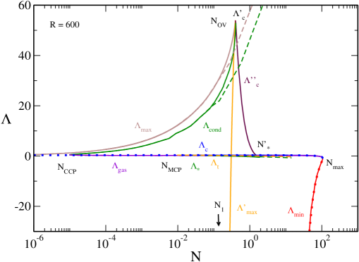
In Fig. 7 we have plotted the caloric curve for . The novelty with respect to the previous case is the existence of a secondary branch presenting an asymptote at . This secondary branch appears suddently at (at that point and ). As detailed in paper1 , for , there exists another equilibrium state at (i.e. ) corresponding to a completely degenerate fermion ball distinct from the ground state. This secondary equilibrium state is unstable.202020Actually, for , there can exist several unstable equilibrium states at (up to an infinity) that have more and more modes of instability. They are related to the spiral structure of the mass-radius relation of the general relativistic Fermi gas at shapiroteukolsky ; paper1 . They give rise to additional branches (with vertical asymptotes) in the caloric curve. We shall not consider these unstable solutions here, except for the less unstable one already mentioned. Its mass is larger than the mass of the stable ground state so that . According to the Poincaré theory, all the configurations of the secondary branch are unstable.212121The spiral present on the left of this secondary branch will ultimately become the cold spiral of Refs. roupas ; paper2 when will be sufficiently large (see below). Therefore, the presence of this secondary branch does not qualitatively change the description of the caloric curve made in Sec. V.2.

However, for , relativistic effects start to become important. This has some consequences on the interpretation of the density profiles. In Fig. 8 we have plotted the different density profiles at . We see that the energy density is low for the gaseous state (G) and for the core-halo state (CH) indicating that we are in the nonrelativistic regime. By contrast, the energy density is relatively high for the stable condensed state (C) and for the unstable condensed state (U) indicating that we are in the relativistic regime. The condensed states almost coincide with a general relativistic fermion ball at containing all the mass (see Appendix E.2.1). They are similar to stable and unstable neutron stars ov . At small but finite temperatures, we see in Fig. 8 that the dashed line obtained from the OV theory provides a good fit to the core of the distribution. There is a small atmosphere (containing a little mass) that becomes thinner and thinner as the temperature is reduced.

Remark: In Fig. 7, when the temperature is low enough, we find four solutions. The solutions (G) and (C) are stable (local minima of free energy) while the solutions (CH) and (U) are unstable (saddle points of free energy). Since we have an even number of extrema, this suggests that there is no global minimum of free energy (naively, this results from simple topological arguments if we plot a curve with two minima and two maxima). The stable equilibrium state with the lowest value of free energy may be only metastable, not fully stable. This is consistent with the result of Zel’dovich zel446 who showed that, at , the OV equilibrium states are only metastable. In Fig. 5, when , we find three solutions. The solutions (G) and (C) are stable (local minima of free energy) while the solution (CH) is unstable (saddle point of free energy). Since we have an odd number of extrema, this suggests that the solution with the lowest value of free energy is a global minimum. This is the case in Newtonian gravity ijmpb . However, this is not quite clear in general relativity since the result of Zel’dovich zel446 still applies for . Therefore, the existence of a global minimum of free energy (fully stable state) in general relativity is not trivial and would require a more careful study. Anyway, for practical purposes, metastable states are very relevant (possibly more relevant than fully stable states) so we shall determine all types of stable equilibrium states, disregarding whether they are fully stable or just metastable.
V.4 The case
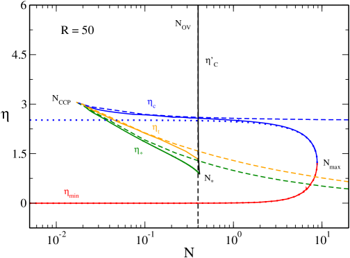
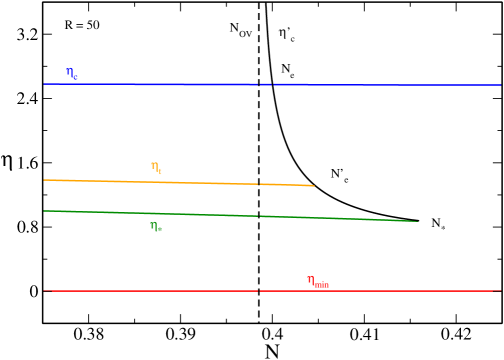
In Fig. 9 we have plotted the caloric curve for . The novelty with respect to the previous case is that the two branches have merged. The merging occurs at at which the two asymptotes and coincide (at that point ). This is the highest value of at which there exist an equilibrium state at (ground state). When there is no equilibrium state at (no ground state) anymore ov . In that case, the caloric curve presents a turning point of temperature at and a turning point of energy at . As a result, there is no equilibrium state at in the canonical ensemble, i.e., below a critical temperature. Similarly, there is no equilibrium state at in the microcanonical ensemble, i.e., below a critical energy. This means that when the system becomes strongly relativistic (i.e. when ) quantum mechanics is not able to prevent gravitational collapse at low temperatures and low energies. This is a generalization of the result first obtained at by Oppenheimer and Volkoff ov in the context of neutron stars.

V.4.1 Microcanonical ensemble
Let us first consider the microcanonical ensemble. The curve is multivalued. According to the Poincaré turning point criterion, the series of equilibria is stable up to and then becomes unstable. The caloric curve presents the following features:
(i) There is no phase transition (there is only one stable equilibrium state for each ).
(ii) There are two regions of negative specific heats, one between and (as before) and another one between (the energy corresponding to ) and . We note that this second region of negative specific heats is extremely tiny. In Fig. 10 we clearly see the convex intruder (dip) associated with the first region of specific heat. The convex intruder associated with the second region of specific heat is imperceptible.
(iii) There is a catastrophic collapse at towards a black hole.222222For simplicity, when there is no equilibrium state, we shall say that the system forms a black hole. Actually, as discussed in Paper II, it is not completely clear that the system will always form a black hole in that case. We leave this interesting problem open to future works.

In Fig. 11 we have plotted the relation between the normalized energy and the central potential. We can see that increases monotonically along the series of equilibria. The curve presents a peak at then displays damped oscillations. These oscillations correspond to the unstable equilibrium states forming the spiral of the caloric curve.

In Fig. 12 we have plotted the relation between the normalized energy and the energy density contrast . We can see that increases monotonically along the series of equilibria up to . Then, on the unstable branch, it displays a more complicated behavior.

The evolution of the system in the microcanonical ensemble is the following. Let us start from high energy states and decrease the energy. As energy decreases, the system becomes more and more concentrated. The central potential and the density contrast increase. If we keep decreasing the energy there comes a point at which the system undergoes a gravitational collapse towards a black hole. This is an instability of general relativistic origin which has no counterpart in the Newtonian theory.
V.4.2 Canonical ensemble
We now consider the canonical ensemble. The function is multivalued. According to the Poincaré turning point criterion, the series of equilibria is stable up to , becomes unstable between and , is stable again between and and becomes unstable again after . The caloric curve presents the following features:
(i) When there are only gaseous states. When there are only condensed states. When there exist gaseous and condensed states at the same temperature. A first order phase transition is expected at a transition temperature determined by the Maxwell construction (see Fig. 9) or by the equality of the free energy of the gaseous and condensed phases (see Fig. 13). When the gaseous states have a lower free energy than the condensed states. When the condensed states have a lower free energy than the gaseous states. However, the first order phase transition does not take place in practice because of the very long lifetime of the metastable states.
(ii) There is a zeroth order phase transition at from the gaseous phase to the condensed phase. It corresponds to a gravitational collapse (isothermal collapse) ultimately halted by quantum degeneracy.
(iii) There is a zeroth order phase transition at from the condensed phase to the gaseous phase. It corresponds to an explosion ultimately halted by the boundary of the box.
(iv) There is a catastrophic collapse at from the condensed phase to a black hole.

In Fig. 14 we have plotted the relation between the inverse temperature and the central potential. We see that increases monotonically along the series of equilibria. The curve presents a first peak at and a second peak at . Then, it displays damped oscillations. They correspond to unstable equilibrium states associated with the spiral of the caloric curve.

In Fig. 15 we have plotted the relation between the normalized inverse temperature and the energy density contrast . We can see that increases monotonically along the series of equilibria up to . Then, on the second unstable branch, it displays a more complicated behavior.

The evolution of the system in the canonical ensemble in the following. Let us start from high temperature states and decrease the temperature. At high temperatures, the system is in the gaseous phase. At , we expect the system to undergo a first order phase transition from the gaseous phase to the condensed phase. However, in practice, this phase transition does not take place because the metastable gaseous states have a very long lifetime. The physical transition occurs at the critical temperature (spinodal point) at which the gaseous phase disappears. At that point the system undergoes a zeroth order phase transition (collapse) from the gaseous phase to the condensed phase. If we keep decreasing the temperature there comes another critical point at which the system undergoes a catastrophic collapse from the condensed phase to a black hole. This is an instability of general relativistic origin which has no counterpart in the Newtonian theory. Inversely, if we increase the temperature, the system displays a zeroth order phase transition (explosion) at from the condensed phase to the gaseous phase.
V.5 The case
In Fig. 16 we have plotted the caloric curve for . The novelty with respect to the previous case is that now is smaller than (they become equal when ).


The description in the microcanonical ensemble is the same as before.
In the canonical ensemble, the caloric curve presents the following features:
(i) When and when there are only gaseous states. When there exist gaseous and condensed states at the same temperature. A first order phase transition is expected at a transition temperature determined by the Maxwell construction (see Fig. 16) or by the equality of the free energy of the two phases (see Fig. 17). When the gaseous states have a lower free energy than the condensed states. When the condensed states have a lower free energy than the gaseous states. However, the first order phase transition does not take place in practice because of the very long lifetime of the metastable states.
(ii) There is a catastrophic collapse at from the gaseous phase to a black hole.
(iii) There is a catastrophic collapse at from the condensed phase to a black hole.
(iv) There is a zeroth order phase transition at from the condensed phase to the gaseous phase. It correspond to an explosion ultimately halted by the boundary of the box.
The evolution of the system in the canonical ensemble is the following. Let us start from high temperature states and decrease the temperature. At high temperatures, the system is in the gaseous phase. At the system is expected to undergo a first order phase transition from the gaseous phase to the condensed phase. However, this phase transition does not take place in practice. At the system undergoes a catastrophic collapse towards a black hole. A condensed phase exists for but it is not clear how it can be reached in practice.
V.6 The case
In Fig. 18 we have plotted the caloric curve for , where is defined such that .


The description in the microcanonical ensemble is the same as before.
In the canonical ensemble, the caloric curve presents the following features:
(i) When and when there are only gaseous states. When there exist gaseous and condensed states at the same temperature. However, there is no first order phase transition, even in theory, because we cannot satisfy the Maxwell construction (see Fig. 18) or the equality of the free energy of the gaseous and condensed phases (see Fig. 19). When the gaseous states always have a lower free energy than the condensed states (see Fig. 19). Therefore, although there are several stable equilibrium states when there is no phase transition from one phase to the other. This is a particularity of the relativistic situation.
(ii) There is a catastrophic collapse at from the gaseous phase to a black hole.
(iii) There is a catastrophic collapse at from the condensed phase to a black hole.
(iv) There is a zeroth order phase transition at from the condensed phase to the gaseous phase. It corresponds to an explosion ultimately halted by the boundary of the box.
The evolution of the system is the same as described previously.
V.7 The case
In Fig. 20 we have plotted the caloric curve for , where is defined such that . From that moment, we denote the minimum energy by instead of .

V.7.1 Microcanonical ensemble
Let us first consider the microcanonical ensemble. The curve is multivalued. According to the Poincaré turning point criterion, the series of equilibria is stable up to and then becomes unstable. The caloric curve presents the following features:
(i) There is no phase transition (there is only one stable equilibrium state for each ).
(ii) There is a region of negative specific heats between and .
(iii) There is a catastrophic collapse at towards a black hole.
The evolution of the system is the same as described previously.
V.7.2 Canonical ensemble
We now consider the canonical ensemble. The function is multivalued. According to the Poincaré turning point criterion, the series of equilibria is stable up to and then becomes unstable. The caloric curve presents the following features:
(i) There is no phase transition (there is only one stable equilibrium state for each ).
(ii) There is a catastrophic collapse at towards a black hole.
The evolution of the system is the same as described previously. The only difference is that the condensed phase has disappeared.
V.8 Larger values of
In Figs. 21 and 22 we have plotted the caloric curves for larger values of . When , the system is nondegenerate and we recover the results of roupas ; paper2 for a classical general relativistic gas described by the Boltzmann distribution.232323As discussed in Sec. XI the classical limit corresponds to and in such a way that is fixed (in more physical terms and with fixed). The caloric curve exhibits a double spiral. When (see Fig. 7 of paper2 ) the two spirals are separated. When (see Fig. 8 of paper2 ) the two spirals are amputed (truncated) and touch each other. When (see Fig. 9 of paper2 ) the spirals disappear and the caloric curve makes a “loop”. When , the caloric curve reduces to a “point” located at .


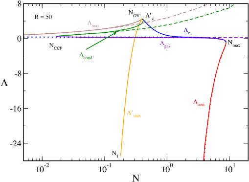
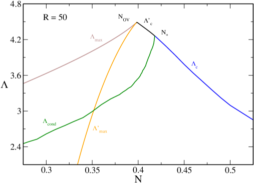
V.9 The canonical phase diagram
In Figs. 23 and 24 we have represented the canonical phase diagram corresponding to (specifically ). It shows the evolution of the critical temperatures , , , , with . We can clearly see the canonical critical point at at which the canonical phase transition appears. We also see the point above which quantum mechanics is not able to prevent gravitational collapse above . Finally, we see the point above which there is no equilibrium state anymore.
The nonrelativistic limit ijmpb corresponds to the dashed lines. It provides a very good approximation of , and for . As we approach general relativity must be taken into account.
The classical limit roupas ; paper2 corresponds to the dotted lines. It provides a very good approximation of (hot spiral) for any . It also provides a very good approximation of (cold spiral) for . As we approach quantum mechanics must be taken into account.
V.10 The microcanonical phase diagram
In Figs. 25 and 26 we have represented the microcanonical phase diagram corresponding to (specifically ). It shows the evolution of the critical energies , , , , , , with . We can clearly see the canonical critical point at at which the region of negative specific heat (associated with the canonical phase transition) appears. We also see the point above which quantum mechanics is not able to prevent gravitational collapse above , and the point above which there is no equilibrium state anymore.
The nonrelativistic limit ijmpb corresponds to the dashed lines. It provides a very good approximation of , and for . As we approach general relativity must be taken into account.
The classical limit roupas ; paper2 corresponds to the dotted lines. It provides a very good approximation of (hot spiral) for any . It also provides a very good approximation of (cold spiral) for . As we approach quantum mechanics must be taken into account.
Remark: we recall that the minimum energy above which equilibrium states exist is (ground state) when and or when . From Fig. 25 we note that increases with while and decrease with . We also note that the system would be a black hole if , i.e., in terms of dimensionless variables. Using Eq. (15), this leads to the condition
| (33) |
One can locate the black hole energy curve in Fig. 25. It behaves as when and as when . It vanishes at and has a maximum at . One can show that the black hole energy curve never intersects the curves of Fig. 25 so that the system is never a black hole (see paper2 for a detailed discussion).
VI The case
We now study the case where the system can display a canonical phase transition (as before) and a microcanonical phase transition (see Fig. 47 below). For illustration we take . In that case, the canonical phase transition appears above and the microcanonical phase transition appears above .
The description of the caloric curves in the canonical ensemble is the same as before. Therefore, in the following, we only consider the microcanonical ensemble. In addition, we focus on what is new and do not treat in detail the situations that are similar to those described previously.
VI.1 The case
VI.2 The case
In Fig. 27 we have plotted the caloric curve for . Since , the caloric curve coincides with the one obtained in the nonrelativistic limit ijmpb . It has a -shape structure leading to a microcanonical phase transition.242424The caloric curve resembles a dinosaur’s neck ijmpb . However, in Fig. 27 the dinosaur has no “chin”. The “chin” appears at as explained in Appendix C.2. The presence, or not, of the “chin” has no physical consequence since it concerns a region of the caloric curve where the equilibrium states are unstable. This -shape structure appears at at which the caloric curve presents a vertical inflexion point. The caloric curve continues up to (outside the frame of the figure) at which it presents an asymptote.

The curve is multivalued leading to the possibility of phase transitions in the microcanonical ensemble. The upper branch up to corresponds to the gaseous phase and the lower branch after corresponds to the condensed phase. According to the Poincaré turning point criterion, these equilibrium states are stable while the equilibrium states on the intermediate branch between and are unstable. The caloric curve presents the following features:
(i) When there are only gaseous states. When there are only condensed states. When there exist gaseous and condensed states with the same energy. A first order microcanonical phase transition is expected at a transition energy determined by the Maxwell construction (see Fig. 27) or by the equality of the entropy of the gaseous and condensed phases (see Fig. 18 of ijmpb ). When the gaseous states have a higher entropy than the condensed states. When the condensed states have a higher entropy than the gaseous states. However, the first order phase transition does not take place in practice because of the very long lifetime of the metastable states.
(ii) There is a zeroth order phase transition at from the gaseous phase to the condensed phase. It corresponds to a gravitational collapse (gravothermal catastrophe) ultimately halted by quantum degeneracy.
(iii) There is a zeroth order phase transition at from the condensed phase to the gaseous phase. It corresponds to an explosion ultimately halted by the boundary of the box.
(iv) There are two regions of negative specific heats, one between and and another one between and .
The evolution of the system in the microcanonical ensemble is the following. Let us start from high energies and decrease the energy. At high energies, the system is in the gaseous phase. At we expect the system to undergo a first order phase transition from the gaseous phase to the condensed phase. However, in practice, this phase transition does not take place because the metastable gaseous states have a very long lifetime. At the system collapses towards the condensed phase. Complete gravitational collapse is prevented by quantum mechanics. The system reaches an equilibrium state similar to a nonrelativistic white dwarf (fermion ball) surrounded by an isothermal atmosphere. If we now increase the energy the system remains in the condensed phase (again, the first order phase transition expected at does not take place because the metastable condensed states have a very long lifetime) until the point at which it explodes and returns to the gaseous phase. We have thus described an hysteretic cycle in the microcanonical ensemble ijmpb .
In Fig. 28 we have plotted the density profiles of the gaseous (G), core-halo (CH) and condensed (C) states at the transition point . We note that the energy density is very low confirming that we are in the nonrelativistic regime. The discussion is essentially the same as in Sec. V.2.3 with the difference that the fermion ball (similar to a nonrelativistic cold white dwarf) that forms in the condensed phase contains only a fraction () of the mass (see ijmpb , Sec. XIII and Appendix E.2.2). The rest of the mass is diluted in a hot halo. This core-halo structure is reminiscent of a red-giant (see Sec. XIII).

VI.3 The case
The second branch with an asymptote at appears at but this does not change the discussion since this branch is made of unstable equilibrium states. From that moment, the system starts to be strongly relativistic.
VI.4 The case
In Fig. 29 we have plotted the caloric curve for .252525We note that the “chin” of the dinosaur has appeared since . The novelty with respect to the previous case is that the two branches have merged. As a result there is no ground state anymore (see Sec. V.4). The caloric curve presents a turning point of energy which corresponds to the minimum energy. When we call it and when we call it (see Sec. V.7 for the definition of ). In the following, to be specific, we assume that but the discussion is essentially the same for .

According to the Poincaré turning point criterion, the series of equilibria is stable up to , becomes unstable between and , becomes stable again between and and becomes unstable again after . The caloric curve presents the following features:

(i) When there are only gaseous states. When there are only condensed states. When there exist gaseous and condensed states with the same energy. A first order phase transition is expected at a transition energy determined by the Maxwell construction (see Fig. 29) of by the equality of the entropy of the gaseous and condensed phases (see Fig. 30). When the gaseous states have a higher entropy than the condensed states. When the condensed states have a higher entropy than the gaseous states. However, the first order phase transition does not take place in practice because of the very long lifetime of metastable states.
(ii) There is a zeroth order phase transition at from the gaseous phase to the condensed phase. It corresponds to a gravitational collapse (gravothermal catastrophe) ultimately halted by quantum degeneracy.
(iii) There is a zeroth order phase transition at from the condensed phase to the gaseous phase. It corresponds to a explosion ultimately halted by the boundary of the box.
(iv) There is a catastrophic collapse at from the condensed phase to a black hole.
(v) There are two regions of negative specific heats, one between and and another one between and .
The evolution of the system in the microcanonical ensemble in the following. Let us start from high energies and decrease the energy. At high energies, the system is in the gaseous phase. At , we expect the system to undergo a first order phase transition from the gaseous phase to the condensed phase. However, in practice, this phase transition does not take place because the metastable gaseous states have a very long lifetime. The physical transition occurs at the critical energy (spinodal point) at which the gaseous phase disappears. At that point the system undergoes a zeroth order phase transition (collapse) from the gaseous phase to the condensed phase. If we keep decreasing the energy there comes another critical point at which the system undergoes a catastrophic collapse from the condensed phase to a black hole. This is an instability of general relativistic origin which has no counterpart in the Newtonian theory. Inversely, if we increase the energy, the system displays a zeroth order phase transition (explosion) at from the condensed phase to the gaseous phase.

In Fig. 31 we have plotted the different density profiles at . We see that the energy density is low for the gaseous state (G) and for the core-halo state (CH) indicating that we are in the nonrelativistic regime. By contrast, the energy density is relatively high for the stable condensed state (C) and for the unstable condensed state (U) indicating that we are in the relativistic regime. The discussion is essentially the same as in Sec. V.3 with the difference that the fermion ball (similar to a general relativistic cold neutron star) that forms in the condensed phase contains only a fraction () of the mass (see Sec. XIII and Appendix E.2.2). The rest of the mass is diluted in a hot halo. This core-halo structure is reminiscent of a supernova (see Sec. XIII).
VI.5 The case
In Fig. 32 we have plotted the caloric curve for . The novelty with respect to the previous case is that now is smaller than (they become equal when ).


The caloric curve presents the following features:
(i) When and there are only gaseous states. When there exist gaseous and condensed states with the same energy. A first order phase transition is expected at a transition energy determined by the Maxwell construction (see Fig. 32) or by the equality of the entropy of the two phases (see Fig. 33). When the gaseous states have a higher entropy than the condensed states. When the condensed states have a higher entropy than the gaseous states. However, the first order phase transition does not take place in practice because of the very long lifetime of the metastable states.
(ii) There is a catastrophic collapse at from the gaseous phase to a black hole.
(iii) There is a catastrophic collapse at from the condensed phase to a black hole.
(iv) There is a zeroth order phase transition at from the condensed phase to the gaseous phase. It corresponds to an explosion ultimately halted by the boundary of the box.
(v) There are two regions of negative specific heats, one between and and another one between and .
The evolution of the system in the microcanonical ensemble is the following. Let us start from high energies and decrease the energy. At high energies, the system is in the gaseous phase. At the system is expected to undergo a first order phase transition from the gaseous phase to the condensed phase. However, this phase transition does not take place in practice. At the system undergoes a catastrophic collapse towards a black hole. A condensed phase exists for but it is not clear how it can be reached in practice.
VI.6 The case
In Fig. 34 we have plotted the caloric curve for , where is defined such that .


The caloric curve presents the following features:
(i) When and when there are only gaseous states. When there exist gaseous and condensed states with the same energy. However, there is no first order phase transition, even in theory, because we cannot satisfy the Maxwell construction (see Fig. 34) or the equality of the entropy of the gaseous and condensed phases (see Fig. 35). When the gaseous states always have an entropy higher than the condensed states. Therefore, although there are several stable equilibrium states when there is no phase transition from one phase to the other. This is a particularity of the relativistic situation.
(ii) There is a catastrophic collapse at from the gaseous phase to a black hole.
(iii) There is a catastrophic collapse at from the condensed phase to a black hole.
(iv) There is a zeroth order phase transition at from the condensed phase to the gaseous phase. It corresponds to an explosion ultimately halted by the boundary of the box.
(v) There are two regions of negative specific heats, one between and and another one between and .
The evolution of the system is the same as described previously.
VI.7 The case
In Fig. 36 we have plotted the caloric curve for , where is defined such that . From that moment, we denote the minimum energy by instead of . The novelty with respect to the previous case is that there is no condensed phase anymore. The discussion is the same as in Secs. V.7 and V.8.

VI.8 The microcanonical phase diagram
In Figs. 37 and 38 we have represented the microcanonical phase diagram corresponding to . It shows the evolution of the critical energies , , , , , , , , and with . We can clearly see the canonical critical point at at which the region of negative specific heat (associated with the canonical phase transition) appears and the microcanonical critical point at at which the microcanonical phase transition appears. We also see the point above which quantum mechanics is not able to prevent gravitational collapse above or . Finally, we see the point above which there is no equilibrium state anymore.
The nonrelativistic limit ijmpb corresponds to the dashed lines. It provides a very good approximation of , , , , , and for . As we approach general relativity must be taken into account.
The classical limit paper2 corresponds to the dotted lines. It provides a very good approximation of (hot spiral) for any . It also provides a very good approximation of (cold spiral) for . As we approach quantum mechanics must be taken into account.
Remark: From Fig. 37 we note that increases with while , and decrease with .
VII The case
For very large radii (), a spiral, winding then unwinding, appears in the caloric curve at the location of the “head” of the dinosaur (this is similar to Fig. 22 of ijmpb and Fig. 44 of clm2 ). However, this spiral is made of unstable states. Therefore, if we restrict ourselves to stable equilibrium states, this mathematical complication (the proliferation of unstable states associated with the spiral) does not change the previous discussion.
Remark: The equilibrium states that are deep in the spiral have a pronounced “core-halo” structure with a large central density (see Fig. 45 of clm2 ). These core-halo states correspond to the configurations computed by Bilic et al. btv and, more recently, by Ruffini et al. rar and Chavanis et al. clm2 . They consist in a large nondegenerate isothermal atmosphere harboring a small “fermion ball”. These solutions look very attractive at first sight because they could provide a self-consistent model of DM halos in which the fermion ball would mimic the presence of a supermassive black hole at the centers of the galaxies (an idea originally proposed in btv ). However, as argued in clm2 , these extreme core-halo structures are thermodynamically unstable (see Secs. VI-VIII of clm2 for a detailed discussion).262626By contrast, less extreme core-halo configurations, such as the solution (CH) computed in Fig. 6, can be stable in the microcanonical ensemble. They have a negative specific heat. These core-halo states are dynamically (Vlasov) stable meaning that if we artificially prepare the system in such a state, it will remain in this state for a long time. However, since these extreme core-halo states are thermodynamically unstable, they are very unlikely (from a thermodynamical point of view) to appear spontaneously. The fermion ball is like a “critical droplet” in nucleation processes. This may be a problem for the fermion ball scenario to mimic the effect of a black hole, as mentioned in clm2 . Other problems with the fermion ball scenario are pointed out in genzel .
VIII The case
We now study the case where there is no phase transition (see Fig. 47 below). In this section, we assume so that and are relatively well separated. For illustration, we take .
VIII.1 The case
VIII.2 The case
In Fig. 39 we have plotted the caloric curve for . The difference with the case treated in Sec. V.3 is that there is no canonical phase transition. The caloric curve is monotonic272727We see a sort of inflexion of the curve which signals the canonical first order phase transition that appears at larger radii . and presents an asymptote at . There is another branch presenting an asymptote at but it is made of unstable states. The series of equilibria of the main branch is stable in both ensembles. The specific heat is always positive. There is no phase transition and no gravitational collapse. The ensembles are equivalent.

VIII.3 The case
In Fig. 40 we have plotted the caloric curve for . The difference with the cases treated in Secs. V.4-V.8 is that there is no phase transition. When the two asymptotes have merged leading to a turning point of temperature at and a turning point of energy at . According to the Poincaré turning point criterion, the series of equilibria is stable up to in the canonical ensemble and up to in the microcanonical ensemble.

In the microcanonical ensemble, the caloric curve presents the following features:
(i) There is no phase transition.
(ii) There is a region of negative specific heats between and .
(iii) There is a catastrophic collapse at towards a black hole.
In the canonical ensemble, the caloric curve presents the following features:
(i) There is no phase transition.
(ii) There is a catastrophic collapse at towards a black hole.
VIII.4 The phase diagrams
In Fig. 41 we have represented the canonical phase diagram corresponding to . It shows the evolution of the critical temperatures and with . We see the point above which quantum mechanics is not able to prevent gravitational collapse above . We also see the point above which there is no equilibrium state anymore.
The classical limit paper2 corresponds to the dotted lines. It provides a very good approximation of (hot spiral) for any . It also provides a very good approximation of (cold spiral) for . As we approach quantum mechanics must be taken into account.
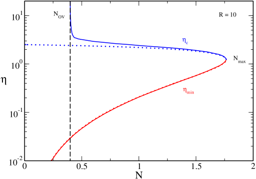
In Fig. 42 we have represented the microcanonical phase diagram corresponding to . It shows the evolution of the critical energies , , and with . We see the point above which quantum mechanics is not able to prevent gravitational collapse above . We also see the point above which there is no equilibrium state anymore.
The nonrelativistic limit ijmpb corresponds to the dashed lines. It provides a very good approximation of for (this is not apparent in the figure but the curves coincide for smaller values of ). As we approach general relativity must be taken into account.
The classical limit paper2 corresponds to the dotted lines. It provides a very good approximation of (hot spiral) for any . It also provides a very good approximation of (cold spiral) for . As we approach quantum mechanics must be taken into account.
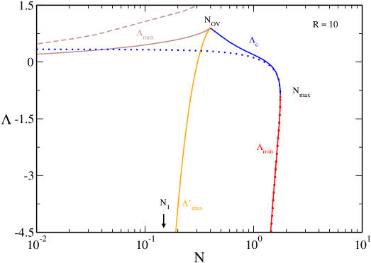
IX The case
We now study the case . In that case, and (see Fig. 47 below).282828We note that for small values of , the values of and (as well as , …) are affected by the presence of the box. This is because the fermion ball at and (ground state) is confined by the walls of the box instead of being self-confined (see paper1 for a detailed study). This is why we have added the letter on these quantities. For illustration, we take .
IX.1 The case
In Fig. 43 we have plotted the caloric curve for . It is similar to that shown in Fig. 4. Since is close to (see below), we clearly see the hot spiral that was outside the frame of Fig. 4. According to the Poincaré turning point criterion, the series of equilibria is stable up to the maximum temperature (corresponding to ) in the the canonical ensemble and up to the maximum energy (corresponding to ) in the microcanonical ensemble. Above and the system collapses into a black hole as discussed in roupas ; paper2 . If we restrict ourselves to small and mid temperatures and energies (as in the preceding sections), there is no phase transition and no gravitational collapse. The specific heat is always positive and the ensembles are equivalent.

IX.2 The case
In Fig. 44 we have plotted the caloric curve for . In that case, we have two asymptotes at and and a turning point of energy and temperature at and . According to the Poincaré turning point criterion, the series of equilibria is stable along the main branch up to the maximum temperature (corresponding to ) in the the canonical ensemble and up to the maximum energy (corresponding to ) in the microcanonical ensemble. As before, if we restrict ourselves to small and mid temperatures and energies, we conclude that there is no phase transition and no gravitational collapse. The specific heat is always positive and the ensembles are equivalent.

IX.3 The phase diagrams
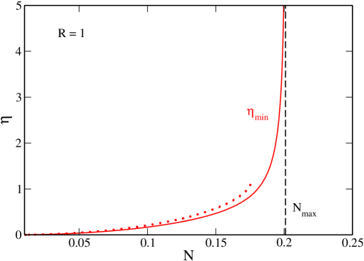
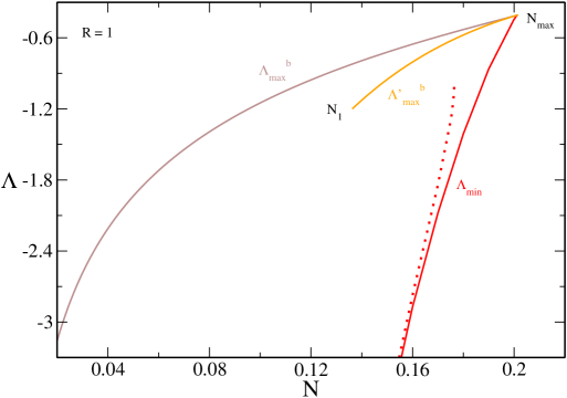
In Fig. 45 we have represented the canonical phase diagram corresponding to . It shows the evolution of the critical temperature with . We note that diverges to when meaning that the caloric curve goes up to infinity and disappears. The classical limit paper2 corresponds to the dotted line. It provides a good approximation for . It is not valid for . This shows that when quantum effects are still important close to . This is because, in the present case, while in the previous examples .
In Fig. 46 we have represented the microcanonical phase diagram corresponding to . It shows the evolution of the critical energies , and with . The classical limit paper2 corresponds to the dotted line. It provides a good approximation for . It is not valid for . When quantum effects are still important close to .
X The phase diagram
We can summarize our results by plotting the characteristic particle numbers encountered in our study as a function of the box radius . This leads to the phase diagram represented in Fig. 47.
X.1 Characteristic particle numbers and characteristic radii
Let us briefly recall the meaning of the characteristic particle numbers appearing on this diagram.292929We present the characteristic particle numbers by order of appearance in the caloric curves as we increase for a given value of . To fix the ideas, we take a large radius so that all kinds of phase transitions are present. We start from a small value of . In that case, the caloric curve is monotonic with an asymptote at corresponding to the stable ground state of the self-gravitating Fermi gas at (). We then increase until we meet the different characteristic particle numbers signaling a topological change of the caloric curve.
(i) When , is the particle number at which the canonical phase transition appears, i.e., the particle number at which and appear in the caloric curve. When , the function is given by the relation obtained in the nonrelativistic study of ijmpb .
(ii) When , is the particle number at which the microcanonical phase transition appears, i.e., the particle number at which and appear in the caloric curve. When , the function is given by the relation obtained in the nonrelativistic study of ijmpb .
(iii) is the particle number at which the unstable equilibrium states at appear, i.e., the particle number at which the second branch with an asymptote at appears in the caloric curve. The function is studied in paper1 . When , the fermion star is self-confined and we have the standard value of the OV theory. When , the fermion star is box-confined and we find that decreases as decreases. When , we find that paper1 .
(iv) is the particle number above which there is no equilibrium state at (no ground state) anymore. At the asymptotes and merge. When they are replaced by a turning point in temperature and by a turning point in energy. The function is studied in paper1 . When , the fermion star is self-confined and we have the standard value of the OV theory. When , the fermion star is box-confined, and we find that decreases as decreases. When , we find that paper1 .
(v) When , is the particle number at which the zeroth order phase transition in the canonical ensemble disappears, i.e., the particle number at which .
(vi) When , is the particle number at which the first order phase transition in the canonical ensemble disappears, i.e., the particle number at which .
(vii) When , is the particle number at which the condensed phase disappears in the canonical ensemble, i.e., the particle number at which .
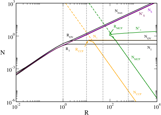
(viii) When , is the particle number at which the zeroth order phase transition in the microcanonical ensemble disappears, i.e., the particle number at which .
(ix) When , is the particle number at which the first order microcanonical phase transition disappears, i.e., the particle number at which .
(x) When , is the particle number at which the condensed phase disappears in the microcanonical ensemble, i.e., the particle number at which .
(xi) When , is the value of the particle number above which the two spirals of the caloric curve are amputed (truncated) and touch each other. When , the function is given by the relation obtained in the classical study of paper2 . When , we find that paper1 . Above that value, the caloric curve looks like Fig. 44 instead of looking like a double spiral.
(xii) When , is the value of the particle number above which there is no spiral anymore and the caloric curve makes a “loop”. When , the function is given by the relation obtained in the classical study of paper2 . When , we find that paper1 .
(xiii) is the maximum particle number below which an equilibrium state may exist for certain values of energy and temperature. For there is no equilibrium state, whatever the energy and the temperature. When , the function is given by the relation obtained in the classical study of roupas ; paper2 . When , we find that paper1 . We note that when while when . The change of regime takes place at where (see the Remark at the end of Sec. IV.3).
X.2 Summary of the main results when is fixed and is varied
The phase diagram exhibits two critical points at and . is the radius above which the system experiences a canonical phase transition when . is the radius above which the system experiences a microcanonical phase transition when . Below, we summarize the essential features of the microcanonical and canonical phase transitions found for the self-gravitating Fermi gas in general relativity. In this section, we consider the situation where is fixed and is varied. We recall that there is a possible equilibrium state only for . We have
| (34) |
| (35) |
As in the previous sections, we do not consider the case of very high energies and very high temperatures which has been treated in roupas ; paper2 .
X.2.1
X.2.2
In the canonical ensemble when , there is no phase transition and no catastrophic collapse. When , there is no phase transition but there is a catastrophic collapse toward a black hole at . When , there is a zeroth order phase transition from the gaseous phase to the condensed phase at and a catastrophic collapse from the condensed phase to a black hole at . When , there is no phase transition but there is a catastrophic collapse from the gaseous phase to a black hole at .
In the microcanonical ensemble, the situation is the same as before.

X.2.3
In the canonical ensemble when there is no phase transition and no catastrophic collapse (see Fig. 4). When there is a zeroth order phase transition from the gaseous phase to the condensed phase at and no catastrophic collapse (see Figs. 5 and 7). When there is a zeroth order phase transition from the gaseous phase to the condensed phase at and a catastrophic collapse from the condensed phase to a black hole at (see Fig. 9). When there is no phase transition but there is a catastrophic collapse from the gaseous phase to a black hole at (see Figs. 16, 18, 20, 21 and 22).
In the microcanonical ensemble, the situation is the same as before.
X.2.4
In the canonical ensemble, the situation is the same as before so we focus on the microcanonical ensemble. When there is no phase transition and no catastrophic collapse. When there is no phase transition but there is a catastrophic collapse towards a black hole at . When there is a zeroth order phase transition from the gaseous phase to the condensed phase at and a catastrophic collapse from the condensed phase to a black hole at or . When there is no phase transition but there is a catastrophic collapse from the gaseous phase to a black hole at .
X.2.5
In the canonical ensemble, the situation is the same as before so we focus on the microcanonical ensemble. When there is no phase transition and no catastrophic collapse. When there is a zeroth order phase transition from the gaseous phase to the condensed phase at and no catastrophic collapse (see Fig. 27). When there is a zeroth order phase transition from the gaseous phase to the condensed phase at and a catastrophic collapse from the condensed phase to a black hole at (see Fig. 29). When there is no phase transition but there is a catastrophic collapse from the gaseous phase to a black hole at (see Figs. 32, 34 and 36).
X.3 Summary of the main results when is fixed and is varied
We now consider the situation where is fixed and is varied.303030This is, for example, the viewpoint adopted by Hertel and Thirring ht as recalled in the introduction (see also Sec. XIII). These results can be deduced from the phase diagram of Fig. 47 by taking the inverse of the functions . This leads to the phase diagram. We note that there is a possible equilibrium state only for where is the inverse function of . We have
| (36) |
| (37) |
X.3.1
In the canonical ensemble when there is no phase transition and no catastrophic collapse. When (with in the nonrelativistic limit ) there is a zeroth order phase transition from the gaseous phase to the condensed phase at and no catastrophic collapse.
In the microcanonical ensemble when (with in the nonrelativistic limit ) there is no phase transition and no catastrophic collapse. When there is a zeroth order phase transition from the gaseous phase to the condensed phase at and no catastrophic collapse.
This is essentially like in the nonrelativistic limit ijmpb . Relativistic corrections occur only close to and/or close to .
X.3.2
In the canonical ensemble when there is no phase transition but there is a catastrophic collapse towards a black hole at . When there is a zeroth order phase transition from the gaseous phase to the condensed phase at and a catastrophic collapse from the condensed phase to a black hole at .
In the microcanonical ensemble when there is no phase transition but there is a catastrophic collapse towards a black hole at . When there is a zeroth order phase transition from the gaseous phase to the condensed phase at and a catastrophic collapse from the condensed phase to a black hole at .
X.3.3
In the canonical ensemble, when there is no phase transition but there is a catastrophic collapse to a black hole at .
In the microcanonical ensemble, the situation is the same as before.
X.3.4
In the canonical ensemble, the situation is the same as before. In the microcanonical ensemble when there is no phase transition but there is a catastrophic collapse towards a black hole at .
XI The nonrelativistic and classical limits
In this section, we consider the nonrelativistic () and classical () limits and study the commutation of these limits.
XI.1 An apparent paradox related to the commutation of the limits and
The commutation of the limits and leads to an apparent paradox. This can be seen from the expression of the maximum OV particle number given by
| (38) |
(i) If we take the nonrelativistic limit first ijmpb , we find that . Therefore, we always have . As a result, there is always an equilibrium state at low temperatures and low energies, whatever the value of , i.e., even if we consider the classical limit .313131In the canonical ensemble, when and , the equilibrium state corresponds to a fermion ball containing most of the mass. When the fermion ball contains all the mass and its radius goes to zero. In that case, we get a Dirac peak of mass (see Appendix E.2.1). In the microcanonical ensemble, when and , the equilibrium state corresponds to a fermion ball containing a fraction of the total mass surrounded by a hot halo. When the mass of the fermion ball and its radius go to zero while its potential energy goes to . As a result, the temperature of the halo goes to . In that case, we get a Dirac peak of zero mass and infinite potential energy (binary) surrounded by an infinitely hot halo (see Appendix E.2.2). Note that for , as small as one pleases, there is always a regular equilibrium state.
(ii) If we take the classical limit first roupas ; paper2 , we find that . Therefore, we always have . As a result, the system undergoes a catastrophic collapse at low temperatures and low energies, whatever the value of , i.e., even if we consider the nonrelativistic limit .
Therefore, if we consider a nonrelativistic classical gas ( and ), the first argument tells us that there is an equilibrium state at low temperatures and low energies while the second argument tells us that there is no equilibrium state at low temperatures and low energies. How can we reconcile these two apparent contradictory situations? In the next two subsections, we re-express these results in terms of dimensionless variables, and in the third subsection we provide a solution of this apparent paradox.
XI.2 When the nonrelativistic limit is taken before the classical limit
In this subsection, we consider the situation where the nonrelativistic limit () is taken before the classical limit (). Using the dimensionless variables of Appendix B, the nonrelativistic limit corresponds to and in such a way that is fixed.323232This scaling is obtained in order to keep the parameter defined in ijmpb fixed (see also Sec. IV.2). Coming back to dimensional variables, the nonrelativistic limit corresponds to and with fixed. This is consistent with the fact that and when . This scaling defines an ensemble of parallel lines of constant in the bottom right panel of Fig. 49. In the nonrelativistic limit, the caloric curves are the same for any couple of points belonging to a given -line. As increases, the -lines move to the right and the system becomes more and more classical ijmpb .
The phase transitions occuring in a nonrelativistic self-gravitating Fermi gas have been studied in ijmpb . When there is no phase transition (see Fig. 14 of ijmpb ). When there is a canonical phase transition (see Fig. 31 of ijmpb ). When there are canonical and microcanonical phase transitions (see Fig. 21 of ijmpb ). The classical limit corresponds to (see Fig. 22 of ijmpb )
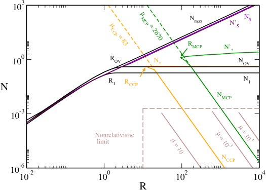

For large but finite values of (see Fig. 50), the series of equilibria forms a spiral which finally unwinds, progresses backward along an inverse spiral until , turns right, forms a lower branch, and finally tends towards an asymptote at where (ground state). When , the direct spiral tends to a limit curve (, ), the inverse spiral coincides with the direct spiral, the turning point is pushed towards , the turning point is pushed towards , the lower branch coincides with the -axis () and the asymptote at is pushed towards . In this limit, we recover the standard nonrelativistic classical caloric curve of Fig. 1 plus a singular branch at corresponding to a Dirac peak of zero mass but infinite potential energy surrounded by a halo of infinite temperature, and a singular branch at corresponding to a Dirac peak containing all the mass (ground state).
XI.3 When the classical limit is taken before the nonrelativistic limit
In this section, we consider the situation where the classical limit () is taken before the nonrelativistic limit (). Using the dimensionless variables of Appendix B, the classical limit corresponds to and in such a way that is fixed.333333This scaling is obtained in order to keep the parameter defined in roupas ; paper2 fixed (see also Sec. IV.3). Coming back to dimensional variables, the classical limit corresponds to and with fixed. This is consistent with the fact that and when . This scaling defines an ensemble of parallel lines of constant in the upper right panel of Fig. 51. In the classical limit, the caloric curves are the same for any couple of points belonging to a given -line. As decreases, the -lines move to the right and the system becomes less and less relativistic roupas ; paper2 .
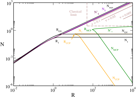
The classical general relativistic self-gravitating gas has been studied in roupas ; paper2 . When the caloric curve displays a double spiral (see Fig. 7 of paper2 ). When the two spirals are truncated (see Fig. 8 of paper2 ). When the caloric curve makes a loop (see Fig. 9 of paper2 ). When the caloric curve reduces to a point and disappears (see Fig. 15 of paper2 ). There is a gravitational collapse at low energies and low temperatures (cold spiral) and at high energies and high temperatures (hot spiral). The nonrelativistic limit corresponds to (see Fig. 12 of paper2 ).


For small but nonzero values of (see Figs. 52 and 53), the series of equilibria forms two spirals very distant to each other. When , the cold spiral tends to a limit curve (, ) while the hot spiral is rejected to the left at infinity ( and ) paper2 . In this limit, we recover the standard nonrelativistic classical caloric curve of Fig. 1 plus a spiral at very high energies and very high temperatures ( and ).
XI.4 The solution of the apparent paradox
In the two processes described previously, in which and , we recover the standard classical nonrelativistic spiral of Fig. 1. However, the manner to obtain it is different depending on the order in which the limits are taken.
When the nonrelativistic limit is taken first, there is no “hot” spiral at since the hot spiral is a general relativity result associated with a form of self-gravitating radiation. By contrast, there is always an asymptote at corresponding to an equilibrium state at (the ground state of the Fermi gas) because . In the classical limit , the asymptote at is rejected at (while is pushed towards and towards zero) so the caloric curve has the form of a single spiral. For infinitely small but finite, we get the classical caloric curve plus singular branches (horizontal) and (vertical) as described previously. According to the results of Appendix E, we have the scalings , and for .
When the classical limit is taken first, there is always a “hot” spiral at since the system is relativistic. By contrast, there is no asymptote at , i.e., there is no equilibrium state at (ground state) because . In the nonrelativistic limit , the “hot” spiral is rejected at infinity so the caloric curve has the form of a single spiral. For infinitely large but finite, we get the nonrelativistic caloric curve plus a spiral at very high energies and temperatures as described previously. According to the results of paper2 (see also footnote 19), we have the scalings and for .
The previous considerations lead to the following conclusion.
The nonrelativistic limit ijmpb corresponds to and . This corresponds to the lower panel QNR of Fig. 54 below . In that case, for a fixed radius , the caloric curve shows no phase transition below , a canonical phase transition above and a microcanonical phase transition (in addition to the canonical phase transition) above . The classical limit corresponds to . This corresponds to the lower right panel CNR1 of Fig. 54 (far on the right) below .
The classical limit roupas ; paper2 corresponds to and . This corresponds to the upper panel CR of Fig. 54 above . In that case, for a fixed radius , the caloric curve shows a double spiral below , a truncated double spiral above , a loop above and no equilibrium states above . The nonrelativistic limit corresponds to . This corresponds to the upper right panel CNR2 of Fig. 54 (far on the right) above .
Therefore, the nonrelativistic classical limit corresponds to two distinct regions in the right panel of Fig. 54, below or above , depending on the order in which the limits are taken. Note also that quantum and relativistic effects are both important only close to or only close to . This corresponds to the region denoted QR in Fig. 54.
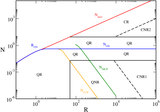
XII Relativistic and quantum corrections
XII.1 Relativistic corrections to the nonrelativistic caloric curves
We have seen in Sec. XI.2 that the nonrelativistic caloric curves of the self-gravitating Fermi gas correspond to parallel lines of constant in the bottom right panel of Fig. 49. On a line of constant , the nonrelativistic limit is valid when and (physically and ). For small values of and large values of , i.e., at the top of a -line, relativistic corrections come into play.
XII.1.1
Let us first consider the case corresponding to (see Figs. 55 and 56). When , we recover the nonrelativistic caloric curve plotted in Fig. 31 of ijmpb . It has a -shape structure leading to canonical phase transitions. The hot spiral is rejected at infinity. Let us increase the number of particles at fixed , hence decreasing the box radius accordingly, in order to see the relativisitic corrections. The description in the change of the caloric curves as relativistic effects become more and more important is qualitatively similar to that given in Sec. V for when . The only difference is that we work at fixed (with ) instead of fixed (with ). Therefore, in the diagram, we follow the oblique line (see Fig. 49) instead of the vertical line (see Fig. 47). As a result, when , we tend towards a limit curve (the nonrelativistic caloric curve with of ijmpb ) which presents a canonical phase transition while in the case studied in Sec. V the canonical phase transition disappears when .
Remark: The characteristic particle numbers described in Sec. X.1 now depend on instead of . They can be obtained by considering the intersection between the curves and the curve with fixed . In this manner, we obtain , , and .
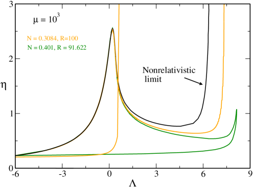
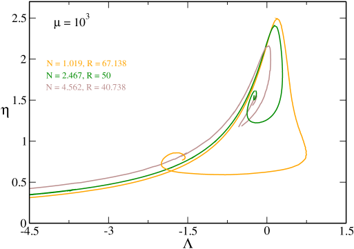
XII.1.2
Let us now consider the case corresponding to (see Figs. 57-59). When , we recover the nonrelativistic caloric curve plotted in Fig. 21 of ijmpb . It has a -shape structure leading to microcanonical phase transitions.343434The resemblance with a dinosaur’s neck in clear on this figure ijmpb . The vertical asymptote at is outside of the frame. The hot spiral is rejected at infinity. Let us increase the number of particles at fixed , hence decreasing the box radius accordingly, in order to see the relativisitic corrections. The description in the change of the caloric curves as relativistic effects become more and more important is qualitatively similar to that given in Sec. VI for when . The only difference is that we work at fixed (with ) instead of fixed (with ). Therefore, in the diagram, we follow the oblique line (see Fig. 49) instead of the vertical line (see Fig. 47). As a result, when , we tend towards a limit curve (the nonrelativistic caloric curve with of ijmpb ) which presents a microcanonical phase transition while in the case studied in Sec. VI the microcanonical phase transition disappears when .
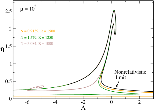
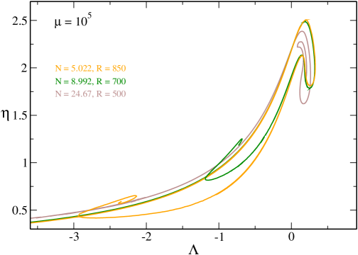
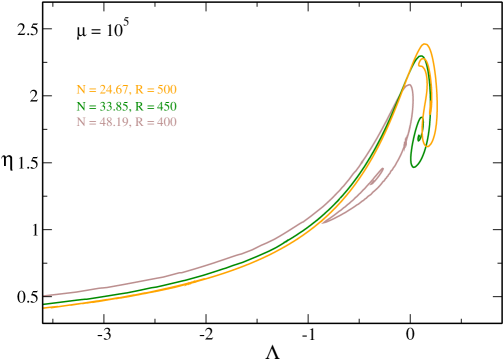
XII.2 Quantum corrections to the classical caloric curve
We have seen in Sec. XI.3 that the classical caloric curves of the general relativistic self-gravitating gas correspond to parallel lines of constant in the upper right panel of Fig. 51. On a line of constant , the classical limit is valid when and (physically and ). For small values of and small values of , i.e., on the left of a -line, quantum corrections come into play.
Let us consider the case (see Figs. 60 and 61). When (black curve) we recover the classical general relativistic caloric curve plotted in Fig. 1 of paper2 . It has the form of a double spiral leading to a gravitational collapse for both cold and hot systems.353535When the caloric curves of Fig. 60 and 61 tend towards a limit curve (the classical general relativistic caloric curve with of paper2 ) which presents a double spiral while in the cases studied in Secs. V-IX the two spirals merge and disappear when . This is because in Secs. V-IX we work at fixed radius while in the present case we work at fixed so that the radius increases as increases. Let us decrease the number of particles at fixed , hence decreasing the box radius accordingly, in order to see the quantum corrections. When (blue and green curves), the caloric curve keeps a similar structure. When (red curve) the caloric curve is made of two branches, each presenting an asymptote (right) and a spiral (left). When (purple curve) the caloric curve has just one branch presenting an asymptote (right) and a spiral (left).
Remark: For smaller values of ,363636This case is specifically investigated in rc . we have a richer variety of caloric curves as decreases with the appearance of canonical and microcanonical phase transitions. This can be seen on the phase diagram of Fig. 51. The characteristic particle numbers described in Sec. X.1 now depend on instead of . They can be obtained by considering the intersection between the curves and the line . In this manner, we obtain and . There is no microcanonical phase transition for and there is no canonical phase transition for .
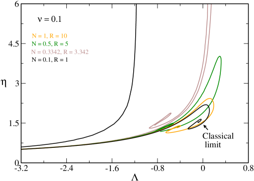
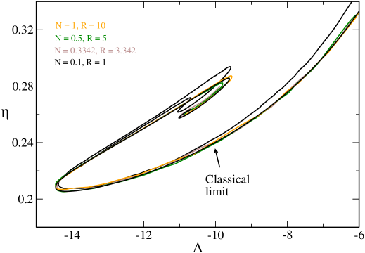
XIII Astrophysical applications
XIII.1 Nonrelativistic model: collapse towards a fermion star
In this section, we discuss astrophysical applications of the nonrelativistic self-gravitating Fermi gas model ijmpb . This model exhibits a phase transition from a gaseous star to a compact fermion star. The fermion star can be a white dwarf, a neutron star or a DM fermion ball.373737In this section we take in the numerical applications. We relate this phase transition to the onset of red-giant structure and to the supernova phenomenon.
XIII.1.1 Canonical ensemble
Let us consider a system of nonrelativistic self-gravitating fermions in the canonical ensemble. The canonical phase transition appears for (canonical critical point) ijmpb hence for
| (39) |
We assume that we are in this situation. In that case, the caloric curve has the form of Fig. 5. The natural evolution proceeds along the series of equilibria towards lower and lower temperatures (see Sec. III). We assume that the system is initially in the metastable gaseous phase. As its temperature decreases it remains in this phase up to the critical point at which the metastable gaseous branch disappears.383838We recall that the collapse takes place at the critical (spinodal) point , not at the transition point , because of the tremendously long lifetime of metastable gaseous states. This critical temperature is not very sensitive on quantum effects (when ) so it can be approximated by its classical value yielding
| (40) |
At that point, the system collapses and forms a compact fermion star. As explained in Appendix E.2.1, in the canonical ensemble, the fermion star contains almost all the mass () and is surrounded by a tenuous atmosphere. If we approximate the fermion star by a Fermi gas at (polytrope of index ) containing all the mass, its radius is given by (see Appendix E.2.1):
| (41) |
The energy of the gaseous phase at the point of isothermal collapse is not very sensitive on quantum effects (when ) so it can be approximated by its classical value yielding
| (42) |
The energy of the condensed object can be approximated by its value at yielding (see Appendix E.2.1):
| (43) |
Finally, the collapse time in the canonical ensemble is of the order of the dynamical time
| (44) |
We note that the collapse in the canonical ensemble corresponds to a pure implosion since almost all the mass is in the condensate (fermion star), not in the halo. The thermodynamical reason for this implosion phenomenon is explained in Appendix E.1. It is also corroborated by the following arguments. If we calculate the density perturbation that triggers the instability at , we find that it has only one node (see Fig. 10 of aa ). Therefore, the instability develops itself in such a way that the density in the core increases while the density in the halo decreases. We also find that the velocity profile has no node (see Fig. 12 of aa ) so that it is purely inward. These two results confirm the implosion phenomenon.
We make below numerical applications to illustrate the preceding results. They correspond to the nonrelativistic models of neutron stars (made of neutrons of mass ) and dark matter halos (made of fermions of mass ) respectively studied by Hertel and Thirring ht and Bilic and Viollier bvn as recalled in the Introduction.
Neutron stars (crude model) ht : We consider a gas of neutrons of total mass .393939The maximum mass and minimum radius of an ideal neutron star set by general relativity are and . Therefore, the value of the mass chosen by ht is larger than the maximum mass. If general relativity were taken into account (see below) the system would not form a neutron star but would collapse towards a black hole (assuming that all the initial mass goes in the compact object). It contains about neutrons. The canonical phase transition appears for . For a gaseous star of size , corresponding to , the collapse temperature is (the transition temperature is ht ). The radius of the neutron star of mass resulting from the collapse of the gaseous star is . The energy of the gaseous star is and the energy of the neutron star is . The energy released during the collapse is . The collapse time is a multiple of which is very short on an astrophysical timescale.404040Note that the prefactor of the collapse time is uncertain and could be of order or larger. As a result, our estimate of the collapse time is not inconsistent with the duration of the supernova phenomenon which can be as short as a few seconds. For supernovae, the energy may be carried quickly by neutrinos. The release of gravitational energy in a supernova () is comparable with the energy of fusion processses which kept the star shining during the first years of its life. However, this takes place in a few seconds (or days) instead of years leading to a huge luminosity. This explains why a star can become as bright as the whole galaxy.
Fermion ball bvn : We consider a gas of DM fermions of total mass .414141This is the typical mass of a DM halo surrounding a baryonic star of mass since the present fraction of baryons and dark matter are and respectively. Here and in the following we consider DM fermions of mass . The maximum mass and minimum radius set by general relativity are and . Since , the nonrelativistic model is justified in that case. The canonical phase transition appears for . For a gaseous halo of size , corresponding to , the collapse temperature is (the transition temperature is bvn ). The radius of the fermion ball of mass resulting from the collapse of the gaseous halo is . The energy of the gaseous halo is and the energy of the fermion ball is . The energy released during the collapse is . The collapse time is a multiple of which is quite long (possibly irrelevant).
Supermassive fermion ball (crude model) bvn : We consider a gas of DM fermions of total mass .424242In that case, general relativity should be taken into account (see below) since . The canonical phase transition appears for . For a gaseous halo of size , corresponding to , the collapse temperature is (the transition temperature is bvn ). The radius of the fermion ball of mass resulting from the collapse of the gaseous halo is . The energy of the gaseous halo is and the energy of the fermion ball is . The energy released during the collapse is . The collapse time is a multiple of , which is very short on a cosmological timescale.
XIII.1.2 Microcanonical ensemble
We now consider a system of nonrelativistic self-gravitating fermions in the microcanonical ensemble. The microcanonical phase transition appears for (microcanonical critical point) ijmpb hence for
| (45) |
We assume that we are in this situation.434343When the whole series of equilibria is stable. When the system evolves, as energy decreases, from the gaseous states to the core-halo states (with a negative specific heat) without instability or phase transition. In that case, the caloric curve has the form of Fig. 27. The natural evolution proceeds along the series of equilibria towards lower and lower energies (see Sec. III). We assume that the system is initially in the metastable gaseous phase. As its energy decreases it remains in this phase up to the critical point at which the metastable gaseous branch disappears.444444We recall that the collapse takes place at the critical (spinodal) point , not at the transition point , because of the tremendously long lifetime of metastable gaseous states. This critical energy is not very sensitive on quantum effects (when ) so it can be approximated by its classical value yielding
| (46) |
At that point, the system collapses and forms a compact fermion star. As explained in Appendix E.2.2, in the microcanonical ensemble, the fermion star contains only a fraction of the total mass () and is surrounded by a massive and very hot atmosphere. If we approximate the fermion star by a Fermi gas at containing a mass , its radius is given by (see Appendix E.2.2):
| (47) |
On the other hand, the temperature of the halo in the condensed phase is given by (see Appendix E.2.2):
| (48) |
From the analytical model developed in pt one finds that the fraction of mass in the core is approximately given by (see Appendix E.2.2):
| (49) |
In many applications, it is sufficient to consider that (see footnote 45). The temperature of the gaseous phase at the point of gravothermal catastrophe is not very sensitive on quantum effects (when ) so it can be approximated by its classical value yielding
| (50) |
The relaxation time depends on the physical process governing the dynamical evolution of the system so it will not be discussed here.
We note that the collapse in the microcanonical ensemble corresponds to an implosion of the core and a heating of the halo. In the box model, the atmosphere is held by the walls of the box. Without the box, it would be expelled at large distances (see Figs. 38 and 41 of clm2 for an illustration in the context of the fermionic King model). Therefore, in the microcanonical ensemble, the collapse leads to the formation of a fermion star and to the expulsion of a hot atmosphere. This core-halo structure is reminiscent of the onset of a red-giant before the white dwarf stage. The implosion of the core and the explosion of the halo is also similar to the supernova phenomenon leading to the formation of a neutron star. These ideas are further developed and illustrated in supernova . The thermodynamical reason for this implosion-explosion phenomenon is explained in Appendix E.1.2. It is also corroborated by the following arguments. If we calculate the density perturbation that triggers the instability at , we find that it has two nodes, corresponding to a core-halo structure (see Fig. 6b of paddyapj ). Therefore, the instability develops itself in such a way that the density increases in the core and in the halo while it decreases between them (the intermediate shell is depopulated). We also find that the velocity profile has one node (see Fig. 4.b of supernova ) so the velocity is directed inward in the core and outward in the halo. These two results confirm the implosion-explosion phenomenon similar to the red-giant structure and to the supernova phenomenon previously described.
We make below numerical applications to illustrate the preceding results.454545In the numerical applications, we have chosen the values of and in order to have . From Fig. 21 of ijmpb we find that . From the relation with , equivalent to Eq. (48), we find that . This can be compared to the approximate value obtained from Eq. (49). The agreement is reasonable in view of the numerous approximations and the logarithmic corrections.
Neutron stars (crude model) ht : We consider a gas of neutrons of total mass . The microcanonical phase transition appears for . For a gaseous star of size the collapse energy is (the transition energy is ). The mass of the neutron star resulting from the collapse of the gaseous star is and its radius is . The temperature of the gaseous star is and the temperature of the halo surrounding the neutron star is .
Fermion ball bvn : We consider a gas of DM fermions of total mass . The microcanonical phase transition appears for . For a gaseous halo of size the collapse energy is (the transition energy is ). The mass of the fermion ball resulting from the collapse of the gaseous halo is and its radius is . The temperature of the gaseous halo is and the temperature of the halo surrounding the fermion ball is .
Supermassive fermion ball (crude model) bvn : We consider a gas of DM fermions of total mass . The microcanonical phase transition appears for . For a gaseous halo of size the collapse energy is (the transition energy is ). The mass of the fermion ball resulting from the collapse of the gaseous halo is and its radius is . The temperature of the gaseous halo is and the temperature of the halo surrounding the fermion ball is .
XIII.2 Relativistic model with : Collapse towards a fermion star
We now consider the truly general relativistic Fermi gas model. We first assume that so that the collapse always leads to a fermion star (not a black hole). The discussion is essentially the same as before. However, we make below new numerical applications to see the effect of relativistic corrections when . These numerical applications are based on the general relativistic models of dark matter halos studied by Bilic and Viollier bvr as recalled in the Introduction.464646In terms of the dimensionless variables defined in Appendix B they take , which is slightly below the OV limit , and . The radius of the completely degenerate fermion ball corresponding to is paper1 . We consider their adaptation to the case of neutron stars. We restrict ourselves to the canonical ensemble.
Supermassive fermion ball bvr : For a fermionic particle of mass the OV limits are , , and . We consider a gas of fermions, corresponding to a rest mass . According to Fig. 47, the canonical phase transition appears for (the nonrelativistic value is ). For a system of initial size , the collapse temperature is (the transition temperature is bvr ). The collapse of the gaseous halo leads to a supermassive fermion ball containing almost all the particles surrounded by a tenuous atmosphere. Since the particle number is slightly below the OV limit, the fermion ball is strongly relativistic. If we approximate the fermion ball by a Fermi gas at containing all the rest mass , we find a radius and a mass paper1 (the nonrelativistic values are and ). The energy of the gaseous halo is and the energy of the fermion ball is (the nonrelativistic value is ). The energy released during the collapse is (the nonrelativistic value is ). The collapse time is a multiple of .
Neutron stars: For the neutrons of mass , the OV limits are , , and . We consider a gas of neutrons, corresponding to a rest mass . The canonical phase transition appears for (the nonrelativistic value is ). For a system of initial size , the collapse temperature is (the transition temperature is ). The collapse of the gaseous star leads to a neutron star containing almost all the particles surrounded by a tenuous atmosphere. Since the particle number is slightly below the OV limit, the system is strongly relativistic. If we approximate the neutron star by a Fermi gas at containing all the rest mass , we find a radius and a mass (the nonrelativistic values are and ). The energy of the gaseous star is and the energy of the neutron star is (the nonrelativistic value is ). The energy released during the collapse is (the nonrelativistic value is ). The collapse time is a multiple of .
Remark: For the value of considered in the previous examples, we find from Fig. 47 that the microcanonical phase transition appears for (the nonrelativistic value is ). Since is below this critical value, the system does not display any phase transition in the microcanonical ensemble.
XIII.3 Relativistic model with : Collapse towards a fermion star followed by a collapse towards a black hole
We now assume that (where and ) so that, by cooling, the system undergoes two successive collapses: a collapse towards a fermion star followed by a collapse towards a black hole.
We consider a system of relativistic self-gravitating fermions in the canonical ensemble. We assume that . The caloric curve has the form of Fig. 9. We assume that the system is initially in the gaseous phase. At its temperature decreases, the system collapses from the gaseous phase to the condensed phase at then undergoes a catastrophic collapse from the condensed phase to a black hole at . We note that the interval is extremely narrow since and for (we see in Fig. 47 that does not change much with ). We have so that
| (51) |
The reason why is easy to understand. We have previously explained that the fermion star contains almost all the particles (). Therefore, as soon as is larger than the fermion star becomes unstable () and collapses towards a black hole (see Appendix G).
We consider a system of relativistic self-gravitating fermions in the microcanonical ensemble. We assume that . The caloric curve has the form of Fig. 29. We assume that the system is initially in the gaseous phase. At its energy decreases, the system collapses from the gaseous phase to the condensed phase at then undergoes a catastrophic collapse from the condensed phase to a black hole at . The interval is much larger than in the canonical ensemble since and for (we see in Fig. 47 that remains in the range ). We have so that
| (52) |
Again, the reason why is easy to understand. We have previously explained that the fermion star contains only a fraction of the particles (). Therefore, if is only slightly larger than , the fermion ball is stable (). It is only when is substantially larger than (by a factor of ) that the fermion ball becomes unstable () and collapses towards a black hole.
XIII.4 Relativistic model with : Direct collapse towards a black hole
We finally assume that so that, by cooling, the system directly collapses towards a black hole, without forming a fermion star.
We consider a system of relativistic self-gravitating fermions in the canonical ensemble. We assume that . The caloric curve has the form of Figs. 16, 18, 20, 21, and 22. We assume that the system is initially in the gaseous phase. As its temperature decreases, the system undergoes a catastrophic collapse from the gaseous phase to a black hole at . This situation corresponds to , where [see Eq. (51)]. This result shows that, in the canonical ensemble, there is no condensed configurations in the general relativisitic Fermi gas at nonzero temperature as soon as is slightly larger than . The reason is that almost of all the particles are in the degenerate core, the rest forming a tenuous isothermal atmosphere.
We consider a system of relativistic self-gravitating fermions in the microcanonical ensemble. We assume that . The caloric curve has the form of Figs. 32, 34 and 36. We assume that the system is initially in the gaseous phase. At its energy decreases, the system undergoes a catastrophic collapse from the gaseous phase to a black hole at . This situation corresponds to , where [see Eq. (52)]. This result shows that, in the microcanonical ensemble, there exist condensed configurations in the general relativisitic Fermi gas at nonzero temperature with . The reason is that only about of the particles are in the degenerate core (so that ), the rest forming an isothermal atmosphere.
XIII.5 Summary
In this section, we summarize the possible evolution of a gaseous star when its temperature (canonical ensemble) or its energy (microcanonical ensemble) is reduced below a critical value.
XIII.5.1 Canonical ensemble
When and , there is no collapse.
When and , the gaseous star collapses below towards a fermion star (white dwarf, neutron star, DM fermion ball). The fermion star contains almost all the mass and is surrounded by a very tenuous atmosphere. Therefore, the collapse corresponds just to an implosion.
When and the gaseous star first collapses below toward a fermion star, then the fermion star collapses below towards a black hole.
When and or when the gaseous star directly collapses towards a black hole.
XIII.5.2 Microcanonical ensemble
When and , there is no collapse.
When and , the gaseous star collapses below towards a fermion star (white dwarf, neutron star, DM fermion ball). The fermion star contains only a fraction of the total mass and is surrounded by a very hot atmosphere. Therefore, the system has a core-halo structure which is similar to the onset of red-giants or to the supernova phenomenon. This core-halo structure results from an implosion of the core and an explosion of the halo.
When and the gaseous star first collapses below toward a fermion star halo, then the fermion star collapses below towards a black hole.
When and or when the gaseous star directly collapses towards a black hole.
XIV Conclusion
In this paper we have studied the nature of phase transitions in the general relativistic Fermi gas. This is the most general situation that we can imagine since both quantum and relativistic effects are taken into account in a rigorous manner. We have obtained the complete phase diagram of the system in the plane (see Fig. 47).
When , the results are similar to those obtained in the nonrelativistic limit (recovered for and with fixed) ijmpb . In that case, there exists an equilibrium state for any value of the temperature and any value of the energy . Catastrophic collapse towards a black hole is prevented by quantum mechanics (Pauli’s exclusion principle). Small systems () do not experience phase transition. Intermediate size systems () experience a canonical phase transition. Large systems () experience canonical and microcanonical phase transitions. A zeroth order phase transition takes place, below a critical temperature or below a critical energy , from a gaseous phase to a condensed phase. The gaseous phase corresponds to a radiative star, a molecular cloud or a primordial DM nebula. The condensed phase corresponds to a compact object (fermion star) such as a white dwarf, a neutron star or a DM fermion ball. In the canonical ensemble the fermion star contains almost all the mass (or is surrounded by a tenuous isothermal atmosphere). The phase transition corresponds to an implosion. In the microcanonial ensemble the compact object contains only a fraction of the total mass ( to fix the ideas) and is surrounded by a hot isothermal atmosphere that contains the remaining mass. Therefore, the condensed phase has a core-halo structure. In the box model the atmosphere is held by the walls of the box. Without the box it would be expelled at large distances. The phase transition corresponds to an an implosion of the core and an explosion of the halo.
When (where in the canonical ensemble and in the microcanonical ensemble), the results are similar to those obtained in the classical limit (recovered for and with fixed) roupas ; paper2 . In that case, there is no condensed phase. Below a critical temperature or below a critical energy , the system undergoes a catastrophic collapse from the gaseous phase to a black hole (presumably). Indeed, quantum mechanics cannot prevent this singularity.
When , the results are new and more complex because the system is both relativistic and quantum. In that case, the system can experience two successive collapses: a zeroth order phase transition at (when ) or (when ) from the gaseous phase to the condensed phase (representing a white dwarf, a neutron star, or a DM fermion ball) followed by a catastrophic collapse at or from the condensed phase to a black hole (presumably). This behavior occurs in a very narrow range of parameters in the canonical ensemble () and in a wider range of parameters () in the microcanonical ensemble.
The previous results apply to mid and low values of energy and temperature. At very high energies and very high temperatures, the system is ultrarelativistic and behaves like a form of self-gravitating radiation. Above a maximum energy or above a maximum temperature , there is no equilibrium state and the system is expected to collapse towards a black hole (presumably) roupas ; paper2 .
The astrophysical applications of our results remain limited by the introduction of an artificial confining box. This is necessary in order to have isothermal equilibrum states with a finite mass and thus investigate phase transitions rigorously. A more astrophysically relevant model with a finite mass is provided by the general relativistic fermionic King model. Phase transitions in the nonrelativistic fermionic King model have been studied in detail in clm1 ; clm2 and give results that are qualitatively similar to those obtained with the box model ijmpb . We believe that similar results would be obtained with the general relativistic fermionic King model.
We have suggested that the microcanonial phase transitions occurring in the self-gravitating Fermi gas may be related to the onset of red-giant structure or to the supernova phenomenon. In these spectacular events, the collapse of the core of the system (resulting ultimately in the formation of a white dwarf or a neutron star) is accompanied by the explosion and the expulsion of a hot envelope.474747Newtonian gravity is sufficient to describe white dwarfs (and the planetary nebula) that follow the red-giant stage while general relativity is necessary to describe neutron stars or black holes formed from supernova explosion. Similarly, in the self-gravitating Fermi gas, the microcanonical phase transition from a gaseous state to a condensed state corresponds to the implosion of the core (leading to a fermion star) and the explosion of the halo. These analogies are further developed in supernova . We may wonder if similar phenomena can occur in the context of DM as suggested in clm2 . It would also be interesting to develop dynamical models of gravitational collapse towards a black hole when no equilibrium state is possible to ensure that the system really forms a black hole. These topics will be considered in future works.
Acknowledgement: One of us (PHC) would like to dedicate this paper to the memory of Donald Lynden-Bell (1935-2018) who was a pioneer in the statistical mechanics of self-gravitating systems.
Appendix A Thermodynamic limit
The thermodynamic limit of nonrelativistic self-gravitating fermions corresponds to in such a way that , and are . Taking , this corresponds to with , , , , and . These scalings are given in htf ; ijmpb . Taking (with ), this corresponds to with , , , , , and .
The thermodynamic limit of relativistic classical self-gravitating systems corresponds to in such a way that , (with ) and are . Taking this corresponds to with , , , , and . To the best of our knowledge, these scalings have not been given previously. Taking (with ) this corresponds to with , , , , , and .
The thermodynamic limit of relativistic self-gravitating fermions corresponds to in such a way that , (with ), and are . Taking this corresponds to with , , , , , and . These scalings were given in bvr . Taking (with ) this corresponds to with , , , , , and .
The thermodynamic limit of nonrelativistic classical self-gravitating systems is discussed in Appendix A of aakin where several possible scalings are given.
We note that the different situations considered above can be unified by considering a thermodynamic limit of the form with , , , , , and , corresponding to (with ). This is the standard thermodynamic limit with a renormalized gravitational constant. To the best of our knowledge this result has not been highlighted previously.
Appendix B Dimensionless quantities
According to the OV theory ov , the maximum mass, the maximum particle number and the minimum radius of a general relativistic fermion star at are484848Qualitatively, the scaling of the maximum mass can be obtained from the mass-radius relation of nonrelativistic fermion stars (see Appendix F) by determining when the radius of the configuration becomes comparable to the Schwarzschild radius .
| (53) |
| (54) |
| (55) |
We note that . We introduce the mass, particle number and length scales
| (56) |
| (57) |
| (58) |
where is the Planck mass and is the Planck length. We then define
| (59) |
| (60) |
| (61) |
| (62) |
where the tilde variables are dimensionless. We note that
| (63) |
| (64) |
In the main text, in order to simplify the notations, we do not write the tildes anymore. This amounts to taking in the dimensional expressions. In particular, we have
| (65) |
| (66) |
| (67) |
Appendix C Connexion between the curves and the caloric curves
In this Appendix, we explain how we obtained the caloric curves of self-gravitating fermions in general relativity following the method given by Bilic and Viollier bvr .494949This Appendix is technical and can be skipped for a first reading. It is nevertheless important to understand where the critical values of (such as , , , etc) obtained in the main text come from.
Let us illustrate this procedure with a simple example. In order to construct the caloric curve corresponding to and (see Fig. 5), we proceed as follows. For a given value of and , we can solve the differential equations (6) and (7) up to and determine from Eq. (10) [we can also determine and with the aid of Eqs. (9), (10), (12) and (16)]. By varying the central potential from to , we can obtain the curve . It is usually nonmonotonic and displays damped oscillations for large values of . As example is represented in Fig. 62 for and (see also Figs. 65 and 66 below).
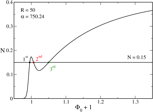

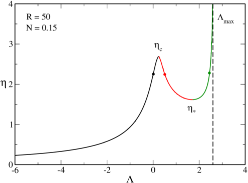
Let us introduce some notations that will be useful in the following. We call the maximum value of the curve and we denote by the value of the central potential corresponding to this maximum. By varying from to , we find that the peaks of the curves reach a maximum at (see Figs. 65 and 66 below). The evolution of as a function of is plotted in Fig. 63.
Let us come back to the curve of Fig. 62. The intersections between the curve and the line level , and the corresponding values of and at these intersections, determine points in the caloric curve of Fig. 64. In the present exemple, . By varying these points form branches in the caloric curve . These branches have been represented in color in Fig. 64. In the present exemple, they correspond to the gaseous, core-halo and condensed phases respectively. We have observed (but not proven mathematically) that when , the merging of two intersections between the curves and the line level , occuring at some , corresponds to the merging of two branches in the caloric curve occurring at an extremum of temperature .505050By using this result, it is easy to obtain the curves , and in the canonical phase diagram of Fig. 23, since they correspond to (see below). Indeed, each extremum of determines an extremum inverse temperature for the corresponding value of . Thus, by considering the first three extrema (when they exist) and running from to , we get the full curves , and . Unfortunately, it is not possible to use a similar method to obtain the curves , , and in the microcanonical phase diagram of Fig. 37. They have to be obtained “by hand” directly from the caloric curves. We have also observed (but not proven mathematically) that when , the merging of two intersections between the curves and the line level , occuring at some , corresponds to the merging of two branches in the caloric curve occurring at an extremum of energy .515151By using this result, it is easy to obtain the curve in the microcanonical phase diagram of Fig. 25, since it corresponds to (see below). Indeed, each extremum of determines an extremum energy for the corresponding value of . Thus, by considering the first extremum and running from to , we get the full curve . Unfortunately, it is not possible to use a similar method to obtain the curve in the canonical phase diagram of Fig. 23. It has to be obtained “by hand” directly from the caloric curves. In the present example, we have . As a result the merging of the first and second intersections in Fig. 62, occurring at some , corresponds to the temperature minimum in the caloric curve of Fig. 64. Similarly, the merging of the second and third intersections in Fig. 62, occurring at some , corresponds to the temperature maximum in the caloric curve of Fig. 64 .
We now generalize this procedure to different values of and . The main difference between the case of classical particles studied in paper2 and the case of fermions studied in the present paper is the following. When quantum mechanics is taken into account, we find that for the curves tend towards an invariant curve correponding to the OV-curve paper1 . Close to this curve, i.e. for large and small, the curves can have a complex behavior with several oscillations responsible for the phase transitions studied in this paper. The nature of these oscillations, and consequently the nature of phase transitions, depends on the particle number and on the radius of the system . We consider below the cases treated in the main text.
C.1
In this subsection, we consider a system of size and make the link between the topological properties of the curves and the caloric curves analysed in Sec. V.
We first consider the case (see Fig. 65). For , we find that and . This corresponds to the ultrarelativistic regime. As increases, increases and decreases: the peak of the curve grows and moves towards the left. At , reaches its maximum value . For larger values of , and both decrease: the peak of the curve decays and moves towards the left. For , and : the peak of the curve is squeezed near .525252Apart from this mathematical property, does not play a particular role in the problem. If we had plotted as a function of instead of [see Eq. (4)] the specificity of the value would not have arisen.
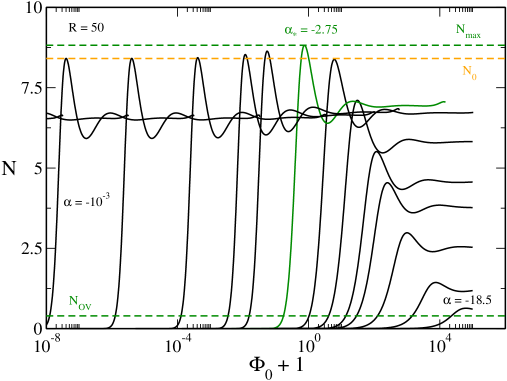
We now consider the case (see Fig. 66). For , we find that decreases and increases: the peak of the curve decays and moves towards the right. For , the curve tends towards the OV-curve : tends towards and tends towards .
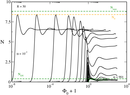
The curves with (i.e. the ones that go up as increases) are associated with the hot spiral (radiation) studied in paper2 . The hot spiral corresponds to the ultrarelativistic limit valid for high values of the energy and of the temperature. This spiral is present for any value of , except for close to where the caloric curve presents a different behavior described in Sec. VI of paper2 and in Sec. IX.2 of the present paper.
The curves with (i.e. the ones that go down as increases) are associated with the part of the caloric curve corresponding to mid and low values of the energy and of the temperature. Figure 67 is a zoom of Fig. 66 close to the OV curve, i.e. for small values of . This is the region of interest where canonical phase transitions appear (they are related to the appearance of turning points of temperature). We have indicated on this figure the different characteristic values of that have been identified in Sec. V. They can be related to the topological properties of the curves as follows:
(i) and are intrinsic properties of the OV curve . They correspond to its first maximum and to its first minimum.
(ii) and can be related to the first and second inflexion points of the curves (see Figs. 68 and 71). Indeed, we have seen that an extremum of temperature in the caloric curve corresponds to a merging of two intersections in the plots. As a result, the canonical phase transitions appear (at ) and disappear (at ) when the curve presents an inflexion point. This is how we can precisely determine and .
Let us now describe in more detail the different intersections as a function of .
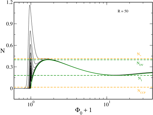
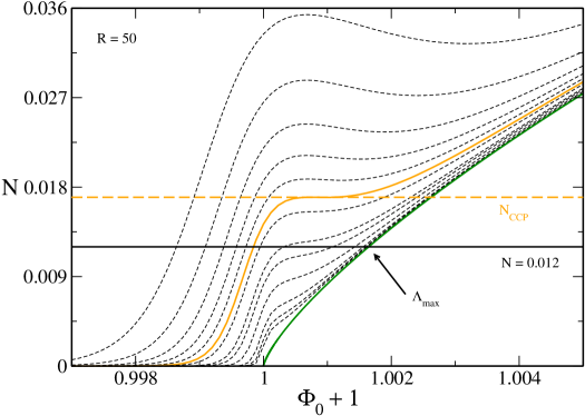
For (see Fig. 68), we have just one intersection between the line level and the curves . This explains why the caloric curve of Fig. 4 is monotonic. We note that the intersection between the line level and the OV-curve () corresponds to the ground state (i.e. ). This leads to the vertical asymptote at in the caloric curve of Fig. 4. We note that, for , showing that we are in the Newtonian limit.
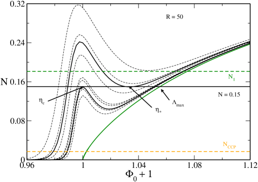
For (see Fig. 69), we are above the first inflexion point so we can have up to three intersections between the line level and the curves . This determines three branches in the caloric curve of Fig. 5. This is why it has an -shape. The first and second intersections merge at . Correspondingly, the first and second branches in the caloric curve merge at , the first turning point of temperature. The second and third intersections merge at . Correspondingly, the second and third branches in the caloric curve merge at , the second turing point of temperature.
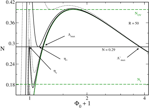
For (see Fig. 70), the novelty is that there is a second intersection between the line level and the OV-curve . This corresponds to an unstable equilibrium state at (i.e. ). This gives rise to the second vertical asymptote at in the caloric curve of Fig. 7. There are also secondary intersections leading to the unstable spiral of Fig. 7 as discussed in the next paragraph.
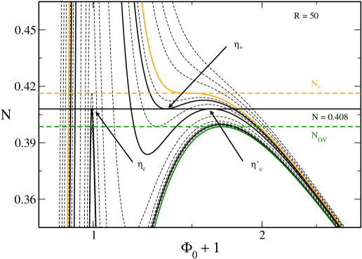
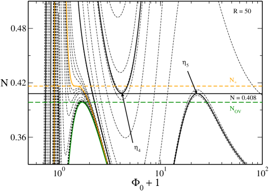
For (see Figs. 71 and 72) we can have up to four fundamental intersections between the line level and the curves . This gives rise to four fundamental branches in the caloric curve of Fig. 16. The first and second intersections merge at . Correspondingly, the first and second branches in the caloric curve merge at , the first turning point of temperature. The second and third intersections merge at . Correspondingly, the second and third branches in the caloric curve merge at , the second turing point of temperature. The third and fourth intersections merge at . Correspondingly, the third and fourth branches in the caloric curve merge at , the third turing point of temperature. Furthermore, there are additional intersections giving rise to the spiral (that will become the cold spiral for larger values of ) in the caloric curve of Fig. 16. These intersections are less relevant since they correspond to unstable states. Note that there is no intersection with the OV curve so there is no vertical asymptote corresponding to . Finally, we note that showing that we are in the relativistic regime.
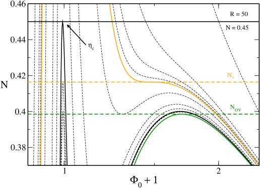
For (see Fig. 73), we are above the second inflexion point so we can have at most two fundamental intersections between the line level and the curves . This determines two fundamental branches in the caloric curve of Fig. 20. The first and second intersections merge at . Correspondingly, the first and second branches in the caloric curve merge , the first turning point of temperature. There are also secondary intersections giving rise to the spiral (made of unstable equilibrium states) as described in the previous paragraph.
For larger values of the discussion is similar to the one given in paper2 .
C.2
We now consider a system of size corresponding to the case analysed in Sec. VI. The novelty with respect to the previous situation is that microcanonical phase transitions can appear (they are related to the appearance of turning points of energy).
Some curves are plotted in Fig. 74 for different values of . We have indicated on this figure the different characteristic values of that have been identified in Sec. VI. As we have seen in the previous section , , , and can be related to the topological properties of the curves . Unfortunately, and cannot be determined from a simple graphical construction because there does not seem to be a simple manner to relate a turning point of energy in the caloric curve to the topological properties of the curves . Therefore, in Sec. VI, we had to determine and “by hand” directly from the study of the caloric curves as a function of .
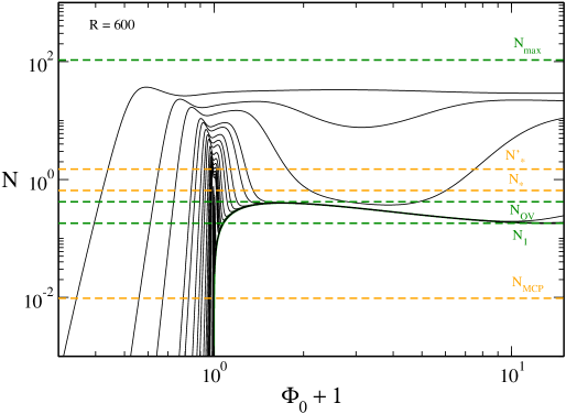
Apart from the occurence of microcanonical phase transitions, there is another novelty with respect to the previous situation (). A new inflexion point appears at (see Fig. 75). For we have two fundamental intersections in the plot leading to two branches of solutions in the caloric curve that merge at the temperature minimum (see Fig. 27).535353In this paragraph, we do not consider the temperature maximum that is far away from the dinosaur’s head. For we have four fundamental intersections in the plot leading to four branches of solutions that merge at the temperature minimum , at the temperature maximum and at the temperature minimum repectively (see Fig. 76). In that case, the dinosaur has a “chin”. This is essentially a curiousity since the solutions in this part of the caloric curve are unstable.
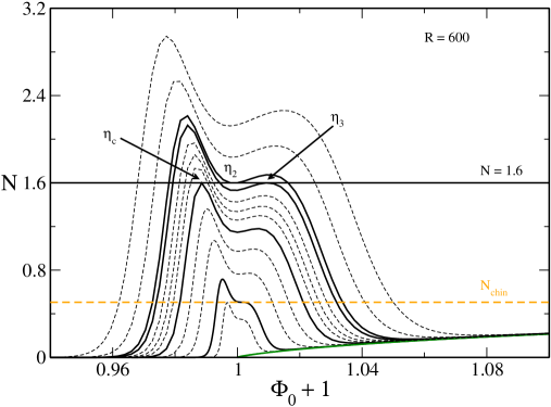

C.3
We consider a system of size corresponding to the case analyzed in Sec. VIII. Some curves are plotted in Figs. 77 and 78 for and respectively. The difference with the case studied in Appendix C.1 is that there is no canonical phase transition. This is manifested by the absence of inflexion points in the family of curves . We also note that, for , is very close to .545454They become equal when corresponding to (see Fig. 63). However, this is essentially a mathematical curiosity without physical consequences.
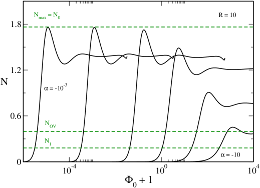
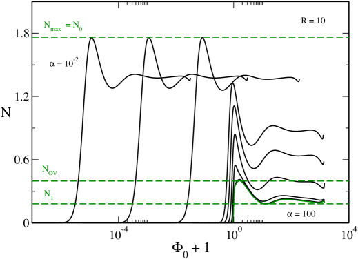
Let us describe the different intersections as a function of . As already mentioned, the intersections with the curves (see Fig. 77) give rise to the hot spiral. This case has already been studied in paper2 . Therefore, we consider below the intersections with the curves (see Fig. 78).
For , we have just one intersection between the line level and the curves . Therefore, the caloric curve is monotonic and is similar to Fig. 4. The intersection between the line level and the OV-curve corresponds to the ground state (i.e. ). This leads to the vertical asymptote at in the caloric curve.
For , there is a second intersection between the line level and the OV-curve . This corresponds to an unstable equilibrium state at (i.e. ). This gives rise to the second vertical asymptote at in the caloric curve of Fig. 39. There are also secondary intersections leading to the cold spiral that is apparent on Fig. 39.
For , there are two fundamental intersections between the line level and the curves . This gives rise to two fundamental branches in the caloric curve of Fig. 40. The first and second intersections merge at . Correspondingly, the first and second branches in the caloric curve merge at , the first turning point of temperature. Furthermore, there are additional intersections giving rise to the cold spiral in the caloric curve of Fig. 40. These intersections are less relevant since they correspond to unstable states. Note that there is no intersection with the OV curve so there is no vertical asymptote corresponding to .
For larger values of the discussion is similar to the one given in paper2 .
C.4
We consider a system of size corresponding to the case analyzed in Sec. IX. Some curves are plotted in Figs. 79 and 80 for and respectively.555555Since , implying , we note that is reached after (see Figs. 79 and 80) while it was reached before in the case (see Figs. 65 and 66). The difference with the previous case is that now is very close to . This is because (see Fig. 63). Therefore is very close to and is very close to .
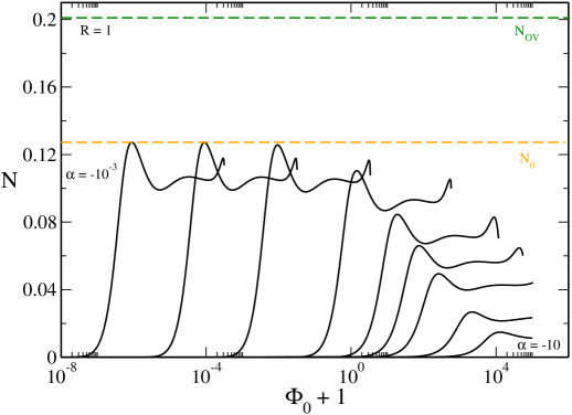
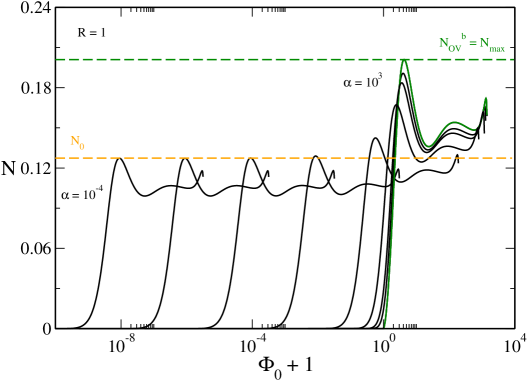
Let us describe the different intersections as a function of (note that most of the curves correspond to ).
For (see Fig. 81), we have one intersection between the line level and the OV-curve which corresponds to the ground state (i.e. ). This leads to the vertical asymptote at in the caloric curve of Fig. 43. In addition, we can have up to an infinity of intersections with the curves leading to the hot spiral displayed in the caloric curve of Fig. 43.
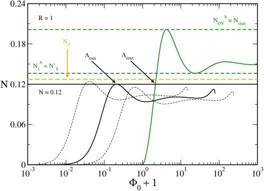
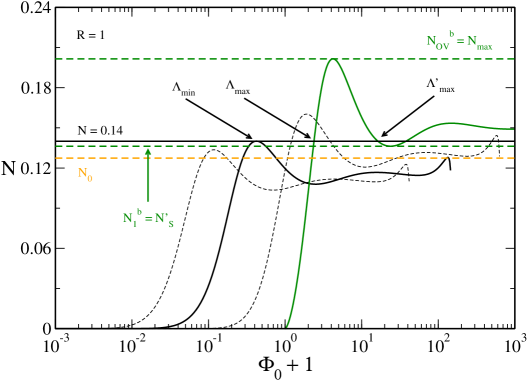
For (see Fig. 82), we have two fundamental intersections between the line level and the OV-curve (corresponding to ) leading to the asymptotes at (stable ground state) and (unstable ground state) in the caloric curve of Fig. 44. For smaller values of , the two fundamental intersections between the line level and the curves lead to two fundamental branches in the caloric curve of Fig. 44. These intersections merge at . Since , this is associated with a turning point of energy at in the caloric curve of Fig. 44. There may also be a third intersection with the OV-curve and secondary intersections with the curves forming a third branch exhibiting an asymptote at and a spiral. However, these solutions are not represented on the caloric curve because they are associated with unstable states of high order.
Appendix D Condition to be degenerate
In the nonrelativistic limit, the system is degenerate when the thermal pressure is small as compared to the quantum pressure arising from the Pauli exclusion principle. This condition can be written as
| (68) |
which is the nonrelativistic Sommerfeld criterion (the right hand side of Eq. (68) is of the order of the Fermi temperature ). To get an estimate of the importance of degeneracy, we replace the density by the average density . In this manner, we obtain the condition
| (69) |
As stated above this condition is only valid in an average sense. A system which does not satisfy this condition in average may still have a degenerate core and a nondegenerate halo as in Appendix E.2.
In the ultrarelativistic limit, the system is degenerate when the thermal pressure is small as compared to the quantum pressure arising from the Pauli exclusion principle. This can be written as
| (70) |
which is the ultrarelativistic Sommerfeld criterion. Proceeding as above, we obtain the condition
| (71) |
where is the OV critical mass given by Eq. (53).
Appendix E Thermodynamics of nonrelativistic self-gravitating systems
In this Appendix, we recall and complete important results concerning the thermodynamics of nonrelativistic self-gravitating systems (classical particles and fermions) that are needed in our analysis. We refer to Appendix F for useful formulae that are used throughout this Appendix.
E.1 Classical particles
We first consider a self-gravitating system of nonrelativistic classical particles confined within a spherical box of radius . We show below that there is no statistical equilibrium state in a strict sense but that long-lived metastable states can exist under certain conditions.
E.1.1 Canonical ensemble
In the canonical ensemble, one can make the free energy diverge towards at fixed mass in the most efficient manner by approaching all the particles at the same point (see Appendix B of sc ). Indeed, let us consider a homogeneous sphere of radius containing all the particles. When the potential energy diverges to . The entropy diverges to but it is subdominant. As a result, the free energy diverges to . Therefore, there is no global minimum of free energy. In a sense, the most probable structure in the canonical ensemble is a Dirac peak containing all the mass.
On the other hand, there exist metastable gaseous states with a temperature lbw ; aa . They have a density contrast lbw ; aa and they are very long-lived lifetime . When , or when and , there are no metastable states anymore and the system collapses (isothermal collapse) aa . According to the previous thermodynamical argument, it is expected to form a Dirac peak containing all the mass. By solving the Smoluchowski-Poisson equations describing the canonical evolution of self-gravitating Brownian particles sc ; post it is found that the Dirac peak is formed in the postcollapse regime of the dynamics.
E.1.2 Microcanonical ensemble
In the microcanonical ensemble, one can make the entropy diverge towards at fixed mass and energy by forming a core-halo structure and letting the size of the core go to zero (see Appendix A of sc ). Indeed, let us consider a homogeneous core made of particles in a sphere of radius . Its potential energy tends to when . In order to conserve the total energy, the kinetic energy of the halo must tend to like meaning that its temperature tends to . As a result, the entropy of the system behaves as and tends to when . Therefore, there is no global maximum of entropy at fixed energy. We note that the divergence of the entropy is the most efficient when the core contains a few particles (). Actually, we only need to approach particles to each other and make a tight binary. Its potential energy diverges towards . The released energy serves to heat the halo made of the other particles. This produces the most efficient divergence of entropy (note that the divergence of entropy is weak — logarithmic). In a sense, the most probable structure in the microcanonical ensemble is a tight binary surrounded by a hot halo. This can be seen as a Dirac peak of zero mass but infinite potential energy a hot halo.
On the other hand, there exist metastable gaseous states with an energy lbw . They have a density contrast antonov ; lbw and they are very long-lived lifetime . When , or when and , there are no metastable states anymore and the system collapses (gravothermal catastrophe) lbw . It is expected to form a binary surrounded by a hot halo. Dynamical models describing the collisional evolution of globular clusters (fluid equations, orbit-averaged Fokker-Planck equation…) show that the binary is formed in the postcollapse regime of the dynamics lbe ; inagaki ; cohn . The energy released by the binary can to stop the collapse and induce a re-expansion of the halo. Then, in principle, a series of gravothermal oscillations should follow oscillations ; hr .
E.2 Fermions
We now consider a self-gravitating system of nonrelativistic fermions confined within a spherical box of radius . In that case, there exists a statistical equilibrium state at any energy and temperature ijmpb . We consider a situation where we are close to the classical limit ( or ). When and there exist metastable gaseous states that are not affected by quantum mechanics (see Appendix E.1). When and there are no metastable states anymore. The system collapses and becomes very dense until quantum mechanics (Pauli’s exclusion principle) comes into play. Generically, the system forms a core-halo structure with a completely degenerate fermionic core of mass and radius surrounded by an (almost classical) isothermal halo of mass and radius . We can obtain the value of from a simple analytical model developed in pt . We summarize this model below by using dimensional variables in order to understand more easily the physical mechanisms at play.
We model the core as a completely degenerate fermion ball. Its mass-radius relation is
| (72) |
Its energy (kinetic potential) is
| (73) |
Its entropy is zero: .
We model the halo by a classical gas at temperature with a uniform density.565656We will see that its temperature is very large in the situations considered. This justifies the uniform density approximation. Its kinetic energy is
| (74) |
Its potential (gravitational) energy, taking into account the presence of the core, is
| (75) |
Its entropy is
| (76) |
In the foregoing expressions, we have assumed which can be checked a posteriori.
The total mass of the system is , its total energy is , its total entropy is and its total free energy is . The mass of the core is obtained by maximizing the entropy at fixed mass and energy in the microcanonical ensemble or by minimizing the free energy at fixed mass in the canonical ensemble. The extremization problem gives in both ensembles pt :
| (77) |
This equation may have several solutions that have been analyzed in detail in pt . Below, we restrict ourselves to the stable condensed state.
E.2.1 Canonical ensemble
In the canonical ensemble, when , we expect that the core contains a large mass (see Appendix E.1.1). Guided by this ansatz, which can be checked a posteriori, one can see from Eq. (E.2) that the core mass is given by
| (78) |
When , the core mass tends towards exponentially rapidly. Therefore the core contains almost all the mass: . Its radius is given by
| (79) |
When , it tends to zero as . The energy of the core is
| (80) |
When , it tends to as . The free energy, which is dominated by the energy of the core, , behaves in a similar manner. In the classical limit , we recover the Dirac peak containing all the mass. This structure leads to the divergence of the free energy in agreement with the arguments of Appendix E.1.1. We note that these results are independent of the presence, or not, of the box.
In terms of dimensionless variables pt , the preceding results can be written as
| (81) |
| (82) |
| (83) |
where . We note that letting (classical limit) in the dimensional equations is equivalent to letting in the dimensionless equations.
Remark: Using the results of Ref. pt , the maximum temperature of the condensed phase, and the corresponding core mass, are given by
| (84) |
Coming back to dimensional variables, we get575757Here and in the following, we give the logarithmic correction in the dominant approximation. Furthermore, should be understood as where is dimensionless.
| (85) |
On the other hand, the temperature of transition, and the corresponding core mass, are given by
| (86) |
Coming back to dimensional variables, we get
| (87) |
E.2.2 Microcanonical ensemble
In the microcanonical ensemble, we expect that the core contains a small mass (see Appendix E.1.2). Guided by this ansatz, which can be checked a posteriori, one can see from Eq. (E.2) that the core mass is given by
| (88) |
When , the core mass tends towards extremely slowly (logarithmically). Therefore, the core contains a fraction of the total mass and this fraction goes to zero as when . The radius of the core is given by
| (89) |
When , it tends to zero as . The energy of the core is
| (90) |
When , it tends to as . Since the energy of the core is very negative the kinetic energy of the halo must be very positive in order to conserve the total energy. It must behave as . Therefore, the temperature of the halo must be very large:
| (91) |
When , it diverges to as . The entropy behaves as . Subtracting the term that we get even in the absence of gravity (see Appendix F), we obtain
| (92) |
When , the entropy diverges to as . In the classical limit , we recover the core-halo structure made of a core having a small mass, a small radius and a huge potential energy (Dirac peak of zero mass) surrounded by a very hot halo.585858We note that the collapse at low energies in the microcanonical ensemble (gravothermal catastrophe) produces hot systems () with a core-halo structure. Actually, although the temperature is uniform throughout the system, the halo is hot while the core is cold. Indeed, the halo is nondegenerate (Boltzmannian) because , where is the Fermi temperature (see Appendix D), while the core is completely degenerate because . Fundamentally, this core-halo structure is the consequence of the negative specific heat of self-gravitating systems as explained in Ref. lbw . This core-halo structure leads to the (logarithmic) divergence of the entropy in agreement with the results of Appendix E.1.2. We note that these results are independent of the presence, or not, of the box. They are also independent of the value of the energy provided that it is not too extreme.
In terms of dimensionless variables pt , the preceding results can be rewritten as
| (93) |
| (94) |
| (95) |
| (96) |
where . More generally (without specifying the value of the core mass ), in the case where the energy of the core tends to and the energy of the halo tends to we have the relation
| (97) |
When is given by Eq. (93) obtained from Eq. (E.2), we recover Eq. (94). Finally, we note that letting (classical limit) in the dimensional equations is equivalent to letting in the dimensionless equations.
Remark: Using the results of Ref. pt , the maximum energy of the condensed phase, and the corresponding core mass, are given by
| (98) |
Coming back to dimensional variables, we get
| (99) |
The energy of transition , and the corresponding core mass , have the same scalings.
Appendix F Useful formulae
In this Appendix, we regroup basic formulae that are useful in our study.
F.1 Energy and entropy
The energy of a nonrelativistic self-gravitating system can be written as
| (100) |
where is the kinetic energy and the potential (gravitational) energy bt .
The Fermi-Dirac entropy functional is given by
| (101) |
where is the maximum allowed value of the distribution function fixed by Pauli’s exclusion principle ptd . In the classical (nondegenerate) limit , it reduces to the Boltzmann entropy functional
| (102) |
The distribution function that maximizes the Boltzmann entropy at fixed density and energy is the Boltzmann distribution
| (103) |
where is the temperature paddy ; aa . Using Eq. (103), the kinetic energy and the entropy of a nonrelativistic classical isothermal self-gravitating system are
| (104) |
and
| (105) |
Remark: We note that the Boltzmann entropy defined by Eq. (102) diverges like when . This divergence is present in the famous Sackur-Tetrode formula for the entropy of a perfect gas (without self-gravity). In order to see the absence of statistical equilibrium states for classical self-gravitating systems, marked by the divergence of the entropy when , we first have to subtract the term from the total entropy (see Appendix E.2.2).
F.2 Homogeneous sphere
The potential (gravitational) energy of a spatially homogeneous sphere of mass and radius is bt :
| (106) |
Using Eqs. (100), (104) and (106), the total energy of a nonrelativistic classical isothermal self-gravitating system with a unifom density is
| (107) |
Using Eq. (F.1) its entropy is
| (108) |
where is the volume of the system.
F.3 Completely degenerate nonrelativistic self-gravitating Fermi gas
The mass-radius relation of a completely degenerate fermion star () in the nonrelativistic limit is
| (109) |
with
| (110) |
where chandrabook .
Its energy (kinetic potential) is chandrabook :
| (111) |
Combined with the mass-radius relation (109), we get
| (112) |
This is the energy of the ground state.
Remark: In terms of dimensionless variables pt , the mass-radius relation can be written as
| (113) |
where and
| (114) |
Similarly, the energy-mass relation can be written as
| (115) |
In writing these expressions, we have implicitly assumed that the fermion star of mass and radius constitutes the core of a larger system of mass and radius as in Appendix E.
F.4 Ground state of a self-gravitating Fermi gas in a box
In terms of dimensionless variables pt , the minimum energy (ground state) of a nonrelativistic self-gravitating Fermi gas enclosed within a box is given by (see Eq. (115) with ):
| (116) |
This expression is valid for a self-confined fermion star such that (i.e., the density of the fermion star vanishes before reaching the box). Using Eq. (113) with , we find that Eq. (116) is valid for . When , the fermion star at (ground state) is box-confined () and its energy is represented in Fig. 2 of ptd .
Introducing the normalized variables of Appendix B and using Eq. (20), we find from Eq. (116) that the minimum energy of a nonrelativistic self-gravitating Fermi gas is given by
| (117) |
This expression is valid for so that the fermion star is self-confined (). This equation can be used to locate the vertical asymptote in the caloric curves of this paper. However, it is only valid in the nonrelativistic regime . In the relativistic regime, the minimum energy of the self-gravitating Fermi gas, as well as the energy of the unstable fermion star at , are represented in Fig. 14 of paper1 . At the point where the second asymptote (corresponding to the unstable fermion star at ) appears, we find that
| (118) |
At the point where the two asymptotes meet each other, we find that
| (119) |
Appendix G Temperature-dependent OV maximum particle number
For and , we find from Fig. 24 that
| (120) |
For a given normalized temperature , the system collapses towards a black hole when , i.e., when with
| (121) |
This can be seen as a temperature-dependent OV maximum particle number. We note that is very close to since (see Sec. XIII.3). The relation (120) remains valid, with a different prefactor, for other values of . On the other hand, for , we have a similar relation for close to (see Fig. 41 for ):
| (122) |
Using the same argument as before, this yields
| (123) |
More generally, writing Eqs. (120) and (122) under the form
| (124) |
we get
| (125) |
If we substitute into Eq. (125) and replace by at leading order, we obtain
| (126) |
We make the guess that the product in Eq. (126) is independent of . This can be checked on the two values that we have computed since the products and are almost the same. As a result, we guess that , i.e., . Substituting this relation into Eq. (126), we finally obtain (using the results of Appendix B):
| (127) |
This relation is expected to be valid for . It gives the first order correction to the OV maximum number due to thermal effects.
References
- (1) T. Padmanabhan, Phys. Rep. 188, 285 (1990)
- (2) V.A. Antonov, Vest. Leningr. Gos. Univ. 7, 135 (1962)
- (3) D. Lynden-Bell, R. Wood, Mon. Not. R. Astron. Soc. 138, 495 (1968)
- (4) P.H. Chavanis, Astron. Astrophys. 432, 117 (2005)
- (5) P.H. Chavanis, Int. J. Mod. Phys. B 20, 3113 (2006)
- (6) G. Alberti, P.H. Chavanis, in preparation
- (7) G. Alberti, P.H. Chavanis, in preparation
- (8) S. Chandrasekhar, An Introduction to the Theory of Stellar Structure (Dover, 1942)
- (9) S.L. Shapiro, S.A. Teukolsky Black Holes, White Dwarfs, and Neutron Stars (Wiley Interscience, 1983)
- (10) N. Bilić, G.B. Tupper, R.D. Viollier, Lect. Notes Phys. 616, 24 (2003)
- (11) H.J. de Vega, P. Salucci, N.G. Sanchez, Mon. Not. R. Astron. Soc. 442, 2717 (2014)
- (12) R. Ruffini, C.R. Argüelles, J.A. Rueda, Mon. Not. R. Astron. Soc. 451, 622 (2015)
- (13) P.H. Chavanis, M. Lemou, F. Méhats, Phys. Rev. D 91, 063531 (2015)
- (14) P.H. Chavanis, M. Lemou, F. Méhats, Phys. Rev. D 92, 123527 (2015)
- (15) V. Domcke, A. Urbano, JCAP 01, 002 (2015)
- (16) L. Randall, J. Scholtz, J. Unwin, Mon. Not. R. Astron. Soc. 467, 1515 (2017)
- (17) P.H. Chavanis, Eur. Phys. J. B 87, 9 (2014)
- (18) Dynamics and thermodynamics of systems with long range interactions, edited by T. Dauxois, S. Ruffo, E. Arimondo, M. Wilkens, Lecture Notes in Physics 602, (Springer, 2002)
- (19) J. Katz, Found. Phys. 33, 223 (2003)
- (20) A. Campa, T. Dauxois, S. Ruffo, Physics Reports 480, 57 (2009)
- (21) A. Campa, T. Dauxois, D. Fanelli, S. Ruffo, Physics of long-range interacting systems (Oxford University Press, 2014)
- (22) P. Hertel and W. Thirring, Commun. Math. Phys. 24, 22 (1971)
- (23) J.M. Lévy-Leblond, J. Math. Phys. 10, 806 (1969)
- (24) P. Hertel, H. Narnhofer and W. Thirring, Commun. Math. Phys. 28, 159 (1972)
- (25) J. Messer, Z. Physik 33, 313 (1979)
- (26) B. Baumgartner, Commun. Math. Phys. 48, 207 (1976)
- (27) P. Hertel, Acta Phys. Austr. Suppl. 17, 209 (1977)
- (28) H. Narnhofer and G.L. Sewell, Commun. Math. Phys. 71, 1 (1980)
- (29) H. Narnhofer and G.L. Sewell, Commun. Math. Phys. 79, 9 (1981)
- (30) W. Braun and K. Hepp, Commun. Math. Phys. 56, 101 (1977)
- (31) P. Hertel and W. Thirring, Thermodynamic Instability of a System of Gravitating Fermions. In: H.P. Dürr (Ed.): Quanten und Felder (Brauschweig: Vieweg 1971)
- (32) J. Messer, J. Math. Phys. 22, 2910 (1981)
- (33) J. Messer, Phys. Lett. 83A, 304 (1981)
- (34) W. Thirring, Z. Physik 235, 339 (1970)
- (35) E.B. Aronson, C.J. Hansen, Astrophys. J. 177, 145 (1972)
- (36) R.D. Carlitz, Phys. Rev. D 5, 3231 (1972)
- (37) S.W. Hawking, Phys. Rev. D 13, 191 (1976)
- (38) P.H. Chavanis, B. Denet, M. Le Berre and Y. Pomeau, preprint
- (39) N. Bilić and R.D. Viollier, Phys. Lett. B 408, 75 (1997)
- (40) P.H. Chavanis, J. Sommeria, Mon. Not. R. Astron. Soc. 296, 569 (1998)
- (41) P.H. Chavanis, Phys. Rev. E 65, 056123 (2002)
- (42) P.H. Chavanis, The self-gravitating Fermi gas, in Dark Matter in Astro- and Particle Physics, edited by H.V. Klapdor-Kleingrothaus and R.D. Viollier (Springer, 2002)
- (43) P.H. Chavanis, I. Ispolatov, Phys. Rev. E 66, 036109 (2002)
- (44) P.H. Chavanis, M. Rieutord, Astron. Astrophys. 412, 1 (2003)
- (45) P.H. Chavanis, Phys. Rev. E 69, 066126 (2004)
- (46) D. Lynden-Bell, Mon. Not. R. Astron. Soc. 136, 101 (1967)
- (47) N. Bilić and R.D. Viollier, Eur. Phys. J. C 11, 173 (1999)
- (48) P.H. Chavanis, G. Alberti, in preparation
- (49) J.R. Oppenheimer, G.M. Volkoff, Phys. Rev. 55, 374 (1939)
- (50) R. Genzel, F. Eisenhauer, S. Gillessen, Rev. Mod. Phys. 82, 3121 (2010)
- (51) N. Bilić and R.D. Viollier, Gen. Rel. Grav. 31, 1105 (1999)
- (52) H. Poincaré, Acta Math. 7, 259 (1885)
- (53) J. Katz, Mon. Not. R. Astron. Soc. 183, 765 (1978)
- (54) J. Katz, Mon. Not. R. Astron. Soc. 189, 817 (1979)
- (55) H. Cohn, Astrophys. J. 242, 765 (1980)
- (56) T. Padmanabhan, Astrophys. J. Supp. 71, 651 (1989)
- (57) P.H. Chavanis, Astron. Astrophys. 381, 340 (2002)
- (58) D. Lynden-Bell, P.P. Eggleton, Mon. Not. R. Astron. Soc. 191, 483 (1980)
- (59) S. Inagaki, D. Lynden-Bell, Mon. Not. R. Astron. Soc. 205, 913 (1983)
- (60) C. Sire, P.H. Chavanis, Phys. Rev. E 69, 066109 (2004)
- (61) Z. Roupas, Class. Quantum Grav. 32, 135023 (2015)
- (62) R.D. Sorkin, R.M. Wald, Z.Z. Jiu, Gen. Relativ. Gravit. 13, 1127 (1981)
- (63) P.H. Chavanis, Astron. Astrophys. 381, 709 (2002)
- (64) P.H. Chavanis, Astron. Astrophys. 483, 673 (2008)
- (65) Ya. B. Zel’dovich, Soviet Physics JETP 15, 446 (1962)
- (66) Z. Roupas, P.H. Chavanis, in preparation
- (67) P.H. Chavanis, Astron. Astrophys. 556, A93 (2013)
- (68) C. Sire, P.H. Chavanis, Phys. Rev. E 66, 046133 (2002)
- (69) D. Sugimoto, E. Bettwieser, Mon. Not. R. Astron. Soc. 204, 19 (1983)
- (70) D. Heggie, N. Ramamani, Mon. Not. R. Astron. Soc. 237, 757 (1989)
- (71) J. Binney, S. Tremaine, Galactic Dynamics (Princeton Series in Astrophysics, 1987)