Can Diffusion Model Achieve Better Performance in Text Generation? Bridging the Gap between Training and Inference!

Zecheng Tang^∗, Pinzheng Wang, Keyan Zhou, Juntao Li, Ziqiang Cao, Min Zhang
Institute of Computer Science and Technology, Soochow University, China
{zctang,pzwang,kyzhou123}@stu.suda.edu.cn;
{ljt,zqcao,minzhang}@suda.edu.cn Equal contribution. Corresponding Author.

Abstract

Diffusion models have been successfully adapted to text generation tasks by mapping the discrete text into the continuous space. However, there exist nonnegligible gaps between training and inference, owing to the absence of the forward process during inference. Thus, the model only predicts based on the previously generated reverse noise rather than the noise computed by the forward process. Besides, the widely-used downsampling strategy in speeding up the inference will cause the mismatch of diffusion trajectories between training and inference. To understand and mitigate the above two types of training-inference discrepancies, we launch a thorough preliminary study. Based on our observations, we propose two simple yet effective methods to bridge the gaps mentioned above, named Distance Penalty and Adaptive Decay Sampling. Extensive experiments on 6 generation tasks confirm the superiority of our methods, which can achieve $\mathbf{100}\times\rightarrow\mathbf{200}\times$ speedup with better performance. Our code is available at https://github.com/CODINNLG/Bridge_Gap_Diffusion.

1 Introduction

With the prevalence of AIGC (Artificial Intelligence Generated Content) in recent years, generative models Kingma and Welling (2013); Goodfellow et al. (2020) have been receiving more attention. As one of the representative generative models, diffusion models Sohl-Dickstein et al. (2015); Song et al. (2020) have achieved great success on myriads of generation tasks with continuous data, such as image Song et al. (2020); Ramesh et al. (2022); Rombach et al. (2022), audio generation Kong et al. (2020), and molecule generation Hoogeboom et al. (2022), by iteratively refining the input noise to match a data distribution. More recently, diffusion models have been successfully adapted to text generation Li et al. (2022); Gong et al. (2022); Lin et al. (2022) by first leveraging an extra embedding module that maps the discrete data into the continuous space and then recovering the text from the continuous space with rounding strategy Li et al. (2022) or logits projection Strudel et al. (2022).

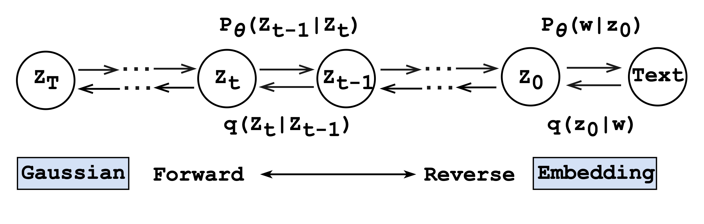
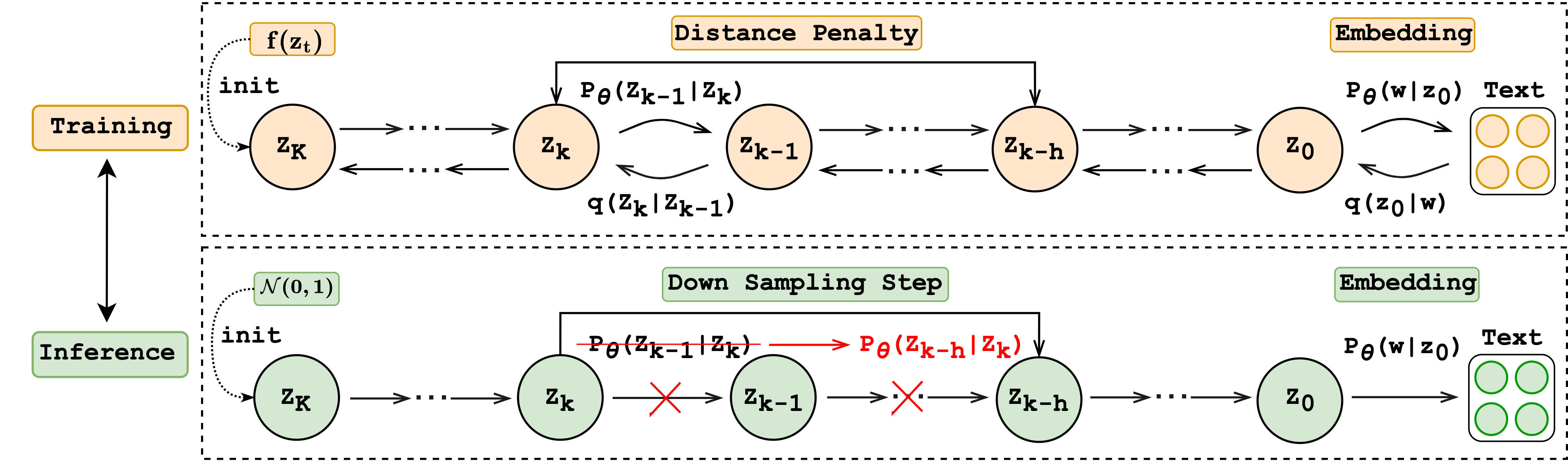
A typical diffusion-based text generation model contains one reverse process (from noise to data) and one forward process (from data to noise), which is shown in Figure 1. More concretely, both of the two processes can be viewed as Markov chains, where the forward process gradually perturbs the data into Gaussian Noise while the reverse process recovers the original data step by step conditioned on the correlated noise from the forward process. The training stage involves both of the above two processes, while the inference stage only consists of the reverse process, i.e., the model predicts based on the previous noise outputted by the model itself rather than the correlated forward noise. Such discrepancy between training and inference, also called exposure bias Ranzato et al. (2015), leads to error accumulation as the denoising steps grow during the inference stage Huszár (2015); Wiseman and Rush (2016).

Refer to caption — Figure 1: Overview of diffusion model for text generation, where $z_{t}$ denotes the intermediate noise at step $t$ .

Another drawback of the diffusion model is that it requires multiple iterative denoising steps to produce the final results since the reverse process should approximate the forward process Ho et al. (2020), which usually involves thousands of steps. Numerous iterative reverse steps of diffusion models are inevitably time-consuming for text generation. For instance, a diffusion model takes around 12 hours on one single NVIDIA A100 GPU to finish the inference of 10K sentences with a length of 128 while the CMLM-based non-autoregressive model Ghazvininejad et al. (2019) only takes a few minutes¹¹1Both diffusion model and CMLM model share the same backbone model, i.e., Transformer Vaswani et al. (2017).. To accelerate the inference speed in text generation, down sampling Nichol and Dhariwal (2021) is leveraged Li et al. (2022); Gao et al. (2022); Gong et al. (2022), though much faster but at the cost of performance owing to the gap between the downsampled steps in inference and the full diffusion trajectory in the training stage.

To explore the insights and the potential improvement of the aforementioned training-inference gaps, we conduct a preliminary study with a diffusion model Gong et al. (2022) on the story generation task and mainly observe that: (1) injecting the noise generated by the model itself into the training stage can improve the model performance, and (2) the uniform downsampling strategy in the inference that treats each step equally impairs the model performance, and adaptive sampling strategy should be applied for different generation stages. Accordingly, we propose two simple yet effective strategies: Distance Penalty and Adaptive Decay Sampling, to bridge the training-inference gaps and accelerate the inference process. Experiments on 6 generation tasks of 3 different settings (directed, open-ended, and controllable) show the superiority of our methods without changing the original architecture of the diffusion model or adding more parameters. Surprisingly, our methods can achieve $\mathbf{100}\times$ speedup with performance improvement or $\mathbf{200}\times$ acceleration with competitive results.

2 Background

2.1 Diffusion Model

Diffusion models are one of the prevalent generative models Sohl-Dickstein et al. (2015); Song et al. (2020); Nichol and Dhariwal (2021), which can transfer an arbitrary data distribution into the Gaussian noise with the forward process and recover the data from the pure noise with the reverse process and both two processes can be regarded as a Markov chain. Specifically, given the time steps $\mathcal{T}=\{0,1,\cdots,T\}$ and the original data distribution $z_{0}$ at time step $t=0$ , the forward process gradually perturbs it into the Gaussian noise $z_{T}\sim\mathcal{N}(0,\mathbf{I})$ at time step $t=T$ :

q(z_{t}\mid z_{t-1})=\mathcal{N}(z_{t};\sqrt{1-\beta_{t}}z_{t-1},\beta_{t}\mathbf{I}),

(1)

where $z_{t}$ represents the intermediate noise at time step $t$ and $\beta_{t}\in(0,1)$ is the scaling factor, controlling the amount of added noise at time step $t$ .

The reverse diffusion process recovers the initial data distribution $z_{0}$ from the Gaussian noise $z_{T}$ by predicting the noise of current time step $t$ and denoising it into the next reverse state $z_{t-1}$ :

p_{\theta}(z_{t-1}\mid z_{t})=\mathcal{N}(z_{t-1};\mu_{\theta}(z_{t},t),\Sigma_{\theta}(z_{t},t)),

(2)

where $\mu_{\theta}$ and $\Sigma_{\theta}$ can be implemented by neural networks $f_{\theta}$ , e.g., Transformer²²2 $\Sigma_{\theta}$ is often set as $\sigma^{2}_{t}\mathrm{I}$ Ho et al. (2020), where $\sigma^{2}_{t}=\beta_{t}$ .:

\mu_{\theta}(z_{t},t)=\frac{1}{\sqrt{\alpha_{t}}}(z_{t}-\frac{\beta_{t}}{\sqrt{1-\bar{\alpha}_{t}}}f_{\theta}(z_{t},t)),

(3)

where $\alpha_{t}=1-\beta_{t}$ and $\bar{\alpha}_{t}=\prod_{i=1}^{t}\alpha_{i}$ .

Training

The training objective of the diffusion model is to maximize the marginal likelihood of data $\log p_{\theta}(z_{0})$ , and the simplified training objective can be written as Ho et al. (2020):

\mathcal{L}_{simple}=\sum\limits_{t=1}^{T}\mathop{\mathbb{E}}\limits_{q(z_{t}\mid z_{0})}||\mu_{\theta}(z_{t},t)-\hat{\mu}({z_{t},z_{0}})||^{2},

(4)

where $\hat{\mu}(z_{t},z_{0})$ is the mean of $q(z_{t-1}\mid z_{0},z_{t})$ , and it is worth noting that each intermediate noise $z_{t}$ can be obtained directly without the previous history during the training stage (Equation 12).

Inference

The inference stage only consists of the reverse process. To sample $z_{t-1}\sim p_{\theta}(z_{t-1}\mid z_{t})$ in Equation 2, reparameterization strategy Kingma and Welling (2013) is leveraged:

z_{t-1}=\mu_{\theta}(z_{t},t)+\sigma_{t}\epsilon,

(5)

where $\epsilon\sim\mathcal{N}(0,\mathbf{I})$ , $\sigma_{t}^{2}=\beta_{t}$ , and $z_{t}$ is initialized with pure Gaussian noise in the beginning. More details about the training and inference stages as well as the derivations are shown in Appendix A.

2.2 Diffusion Model for Text Generation

The core of applying diffusion models for text generation task is the transition between discrete space and continuous space. Existing works mainly introduce the embedding function Li et al. (2022) $\mathcal{E}(\cdot)$ to map the discrete text $\mathbf{w}=\{w_{1},w_{2},\cdots,w_{L}\}$ of length $L$ into the continuous space $\mathcal{E}(\mathbf{w})=\{\mathcal{E}(w_{1}),\mathcal{E}(w_{2}),\cdots,\mathcal{E}(w_{L})\}\in\mathbb{R}^{Ld}$ . Thus, the diffusion model can handle discrete text generation by adding an extra forward step before $t=0$ , denoted as $q(z_{0}\mid\mathbf{w})=\mathcal{N}(\mathcal{E}(\mathbf{w}),\sigma_{0}\mathbf{I})$ , and another step at the end of the reverse process, i.e., $p_{\theta}(\mathbf{w}\mid z_{0})$ . More details are given in Appendix B.

2.3 Inference Speedup

One critical point that prevents the usability of diffusion models in text generation is their slow sampling speed during inference due to the long reverse trajectory, which makes each diffusion step simple and easy to estimate Sohl-Dickstein et al. (2015). To accelerate the inference speed in text generation tasks, current works Li et al. (2022); Gao et al. (2022) apply the downsampling strategy Nichol and Dhariwal (2021) that picks the subset $\mathcal{T}^{\prime}=\{t_{1}^{\prime},t_{2}^{\prime},\cdots,t_{k}^{\prime}\}$ from the full diffusion trajectory and each intermediate reverse step can be obtained by: $z_{t-1}^{\prime}=\mu_{\theta}(z_{t}^{\prime},t^{\prime})+\sigma_{t}^{\prime}\epsilon$ .

3 Gaps between Training and Inference

From the above description of diffusion models, we can summarize two gaps: (1) the reverse process at time step $t$ in inference is conditioned on the predicted noise $z_{t+1}$ by the model itself while $z_{t+1}$ can be obtained directly with the forward computation $q(z_{t+1}\mid z_{0})$ during training, and (2) the downsampled time subset $\mathcal{T}^{\prime}$ in inference is inconsistent with the full diffusion trajectory $\mathcal{T}$ in training stage when applying the downsampling method for inference speedup. To calibrate the effects of these two types of training-inference gaps, we launch a study on the story generation task in this section.

3.1 Study Settings

We implement the diffusion model with the transformer model and select the ROC Stories (ROC) corpus Mostafazadeh et al. (2016) for the story generation task. Specifically, given the prompt or the source sentence $\mathbf{w}^{x}$ and the reference $\mathbf{w}^{y}$ , we apply the partially noising strategy Gong et al. (2022) for training (Appendix A). We utilize BLEU (B-2) score Papineni et al. (2002) to reflect the generation precision (the higher, the better), Lexical Repetition (LR-2) score Shao et al. (2019) to show the diversity of text (the lower, the better), ROUGE (R-2) to represent the recall of generation result (the higher, the better) and Perplexity (PPL) to reflects the fluency (the lower, the better). More implementation details are in Appendix C.

3.2 Analysis

Training with Predicted Noise

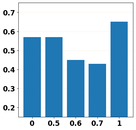
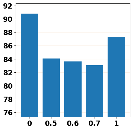
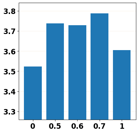
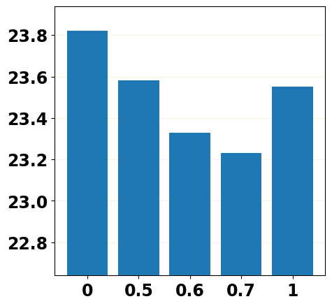
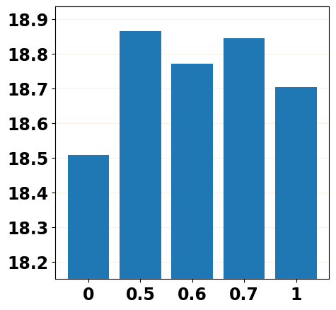
To mitigate the training-inference gap, it is natural to inject part of the predicted noises into the training stage by replacing the forward noise $z_{t+1}$ in $p_{\theta}(z_{t}\mid z_{t+1})$ with the predicted noise $z_{t+1}^{\prime}$ from the $(t+1)$ -th step of the reverse process or injecting the predicted noise into $z_{t}$ by replacing $||\mu_{\theta}(z_{t},t)-\hat{\mu}(z_{t},z_{0})||^{2}$ in Equation 4 with $\gamma_{1}||\mu_{\theta}(z_{t},t)-\hat{\mu}(z_{t},z_{0})||^{2}+\gamma_{2}||\mu_{\theta}(z_{t},t)-\hat{\mu}(z_{t}^{\prime},t)||^{2}$ , where $z_{t}\sim q(z_{t}\mid z_{0})$ and $z_{t}^{\prime}\sim p_{\theta}(z_{t}\mid z_{t+1}^{\prime})$ . We report the evaluation results in Figure 2 with different settings of $\gamma_{1}$ and $\gamma_{2}$ and can mainly observe that replacing the forward noise with the predicted noise ( $\gamma_{2}=1,\gamma_{1}=0$ ) does mitigate the training-inference gap by achieving a better performance than the vanilla training scheme ( $\gamma_{2}=0,\gamma_{1}=1$ ), and the injecting strategy performs better than the replacing one. More details about noise replacement operation and evaluation results are shown in Appendix D.1.

Sampling Strategy

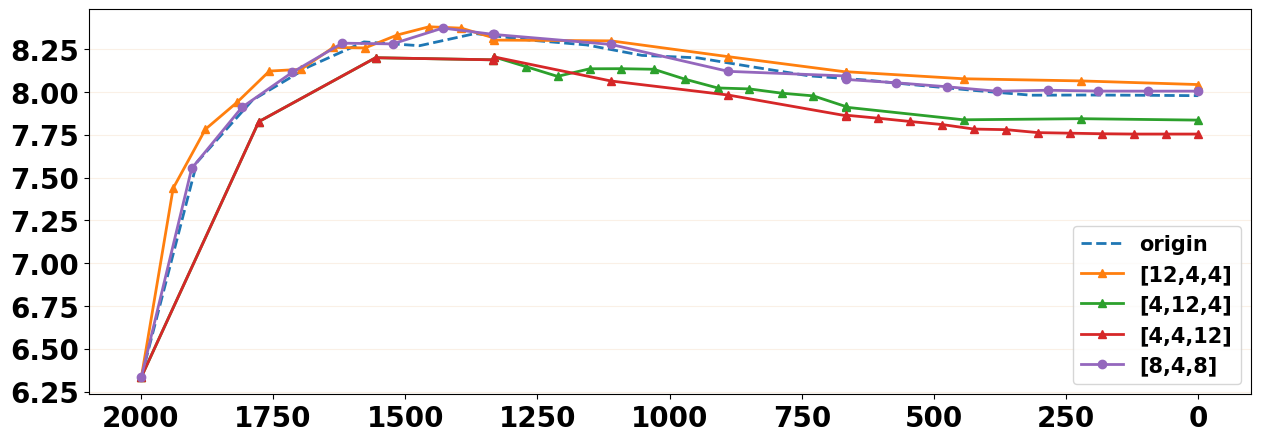
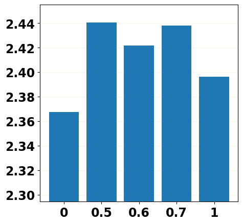
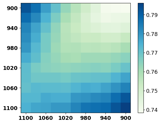
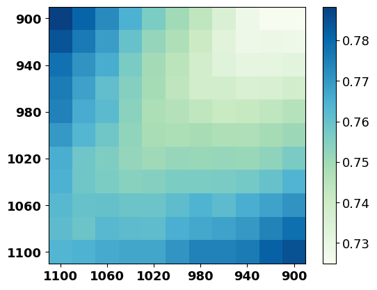
Downsampling can accelerate the inference by uniformly selecting the subsets $\mathcal{T}^{\prime}$ from the full diffusion trajectory $\mathcal{T}$ but at the cost of performance. Such a uniform sampling strategy treats each reverse step equally while neglecting the discrepancies among them in contribution to the final result. To explore whether such an equal-step sampling strategy brings the performance decrease, we simply compare different non-uniform sampling schemes. Along with the reverse steps, we split the reverse process into three stages $[\kappa_{1},\kappa_{2},\kappa_{3}]$ and downsample different numbers of steps for each stage but keep the total downsampled steps the same³³3For total number of downsampled steps 20, we can sample $\{[12,4,4],[4,12,4],[4,4,12],[8,4,8]\}$ steps as $[\kappa_{1},\kappa_{2},\kappa_{3}]$ .. As shown in Figure 3, we can observe that when downsampling more steps from $\kappa_{1}$ (orange curve), the model can achieve a better performance than other downsampling schemes (green curve, red curve, and purple curve) and even exceed the original full reverse steps (blue curve). In other words, the equal-step uniform downsampling scheme does limit the model capability, and the simple non-uniform downsampling strategy can mitigate such issue and meanwhile accelerate the inference speed.

Extensive Trials

As mentioned above, the gap brought by the different diffusion trajectories in the inference stage, i.e., downsampled reverse steps v.s. the full reverse steps, further aggravates the training-inference discrepancy. In view that simply injecting the predicted reverse noise in training can effectively narrow the gaps between training and inference, it is also appealing to make such a strategy adapt to the downsampled diffusion trajectories, i.e., introducing the downsampled reverse noises in the training stage. 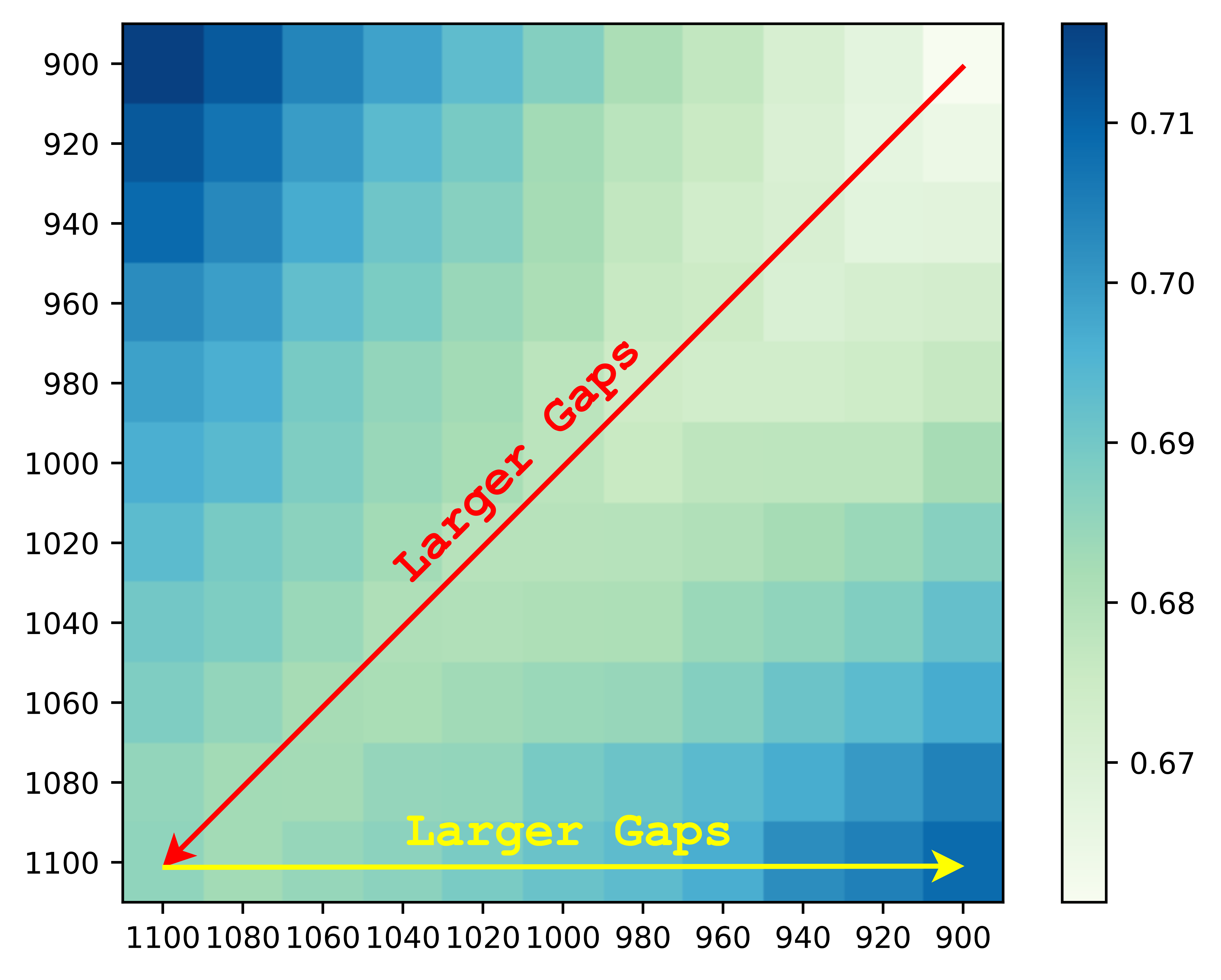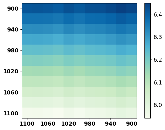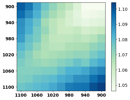For instance, we can inject the predicted reverse noise downsampled from the reverse steps of $(t,t+\delta]$ into the $d$ -th ( $d\sim(t,t+\delta]$ ) forward noise to compute the $t$ -th step reverse noise, i.e., replacing the forward noise $z_{t+1}$ in $p_{\theta}(z_{t}\mid z_{t+1})$ with $z_{d\sim(t,t+\delta]}$ .

Intuitively, adding a perturbation with a reasonable range of values in training can make the model more robust towards the perturbation during inference, while an unconstrained perturbation value might risk the model training, e.g., the training collapse in auto-regressive text generation models Zhang et al. (2019b). For our purposes, the discrepancy before and after injecting the downsampled reverse noise in each training step should fall in a rational range, which mainly depends on the time step $t$ and the choice of $\delta$ . To explore more insights, we depict the discrepancy between predicted reverse noises and forward noises along with 200 randomly selected continuous time steps with the Euclidean distance, which is consistent with the training objective in Equation 4. To simplify the study experiment, we downsample a time step for every twenty steps⁴⁴4We utilize the diffusion model trained with 240K steps. More implementation details are shown in Appendix D.2. As shown in Figure 4, we can observe that (1) the discrepancy between predicted reverse noises and forward noises is getting larger along with the increase of time step $t$ (red diagonal arrow), and (2) the differences between the forward noise at time step $t$ and the predicted reverse noise from $t$ to $t+\delta$ are becoming larger along with the increase of time step (yellow horizontal arrow). Thus, the range of downsampled reverse noise steps should be gradually narrowed along with the increase of time step.

3.3 Potential Improvement

Based on the analysis mentioned above, we can conclude that: (1) injecting the predicted reverse noise into the training stage can mitigate the training-inference gaps, (2) the scheme of uniform downsampling in inference which treats each step equally harms the model performance, and a non-uniform adaptive method should be designed, and (3) inspired by (1) and (2), we can inject the downsampled reverse noises into the training stage while the range of downsampled steps should be gradually narrowed as the time step increases.

4 Method

We propose two simple yet effective methods: Distance Penalty in the post-training stage and Adaptive Sparse Sampling in inference to bridge the gaps without introducing any architecture modification to diffusion models. Thus, it can be flexibly adapted to different diffusion model variants.

4.1 Distance Penalty

We first introduce the Distance Penalty strategy, which injects the Downsampled predicted reverse noise into the post-training stage of diffusion models that consists of $T$ time steps.⁵⁵5To make sure each reverse step can generate a rational noise for perturbation, we apply the Distance Penalty strategy to a converged model. We also apply such a strategy in different training stages in Appendix F.4. For better illustration, we utilize new symbols $\mathcal{K}=\{0,1,\cdots,K\}$ for the time steps in the post-training stage to distinguish from the original diffusion trajectory $\mathcal{T}$ in the training stage. The overview of the Distance Penalty strategy is shown in Figure 5.

Downsampling Range in Training

To obtain a rational predicted reverse noise for each step $k$ , i.e., conduct the downsampling operation in the range $\mathcal{R}_{k}=\{k-1,\cdots,k-h\}$ , and mitigate the training-inference gaps, we constrain the total amount of noises in $\mathcal{R}_{k}$ with the threshold $\omega^{k}_{adj}$ :

\omega^{k}_{adj}=\frac{\sqrt{1-\bar{\alpha}_{K}}}{k^{\prime}},

(6)

where $\sqrt{1-\bar{\alpha}_{K}}$ denotes the scaling factor that controls the variance of noise accumulated at step $K$ (Appendix A), and $k^{\prime}$ is the number of the predefined downsampled steps in inference.

Noise Injection

After obtaining the downsampling range $\mathcal{R}_{k}=\{k-1,\cdots,k-h\}$ for step $k$ , we can inject the predicted reverse noise into reverse step $k$ with Equation 12 in Appendix A, by which we can acquire every predicted reverse noise $z_{d\sim\mathcal{R}_{k}}$ with the correlated forward noise $z_{d+1}$ :

\left\{\begin{aligned} &\mathcal{L}_{dis}=\sum\limits_{k=1}^{K}\sum\limits_{h=1}^{|\mathcal{R}_{k}|}||\mu_{\theta}(z_{k},k)-\hat{\mu}(z_{k-h},k-h)||^{2}\\ &z_{k-h}=\mu_{\theta}(z_{k-h+1},k-h+1)+\sigma^{2}_{k-h+1}\mathbf{I},\end{aligned}\right.

(7)

where $\mathbf{I}\sim\mathcal{N}(0,1)$ and $\sigma^{2}_{k-h+1}=\beta_{k-h+1}$ .

However, the random item $\mathbf{I}$ in $z_{k-h}$ makes the model difficult to converge, and the computation of $\mathcal{L}_{dis}$ is complex. Thus, we apply the simplified Equation 15 in Appendix B, which approximates the model output $f_{\theta}(z_{d})$ to the original data distribution directly, and rewrite the loss function into:

\mathcal{L}^{dis}_{simple}=\sum\limits_{k=1}^{K}\sum\limits_{h=1}^{|\mathcal{R}_{k}|}||f_{\theta}(z_{k},k)-f_{\theta}(z_{k-h},k-h)||^{2},

(8)

Considering that the step $k$ is uniformly sampled during the training stage, to avoid the boundary condition $k-h<0$ , the final training objective is:

\mathcal{L}_{post}=\left\{\begin{aligned} &\mathcal{L}_{simple}+\gamma\mathcal{L}_{simple}^{dis}&k\geq h&\\ &\mathcal{L}_{simple}&k<h&,\end{aligned}\right.

(9)

where $\mathcal{L}_{simple}$ is the original training objective of diffusion model (Equation 4), and $\gamma$ is the penalty weight that controls the degree of the constraint.

4.2 Adaptive Decay Sampling

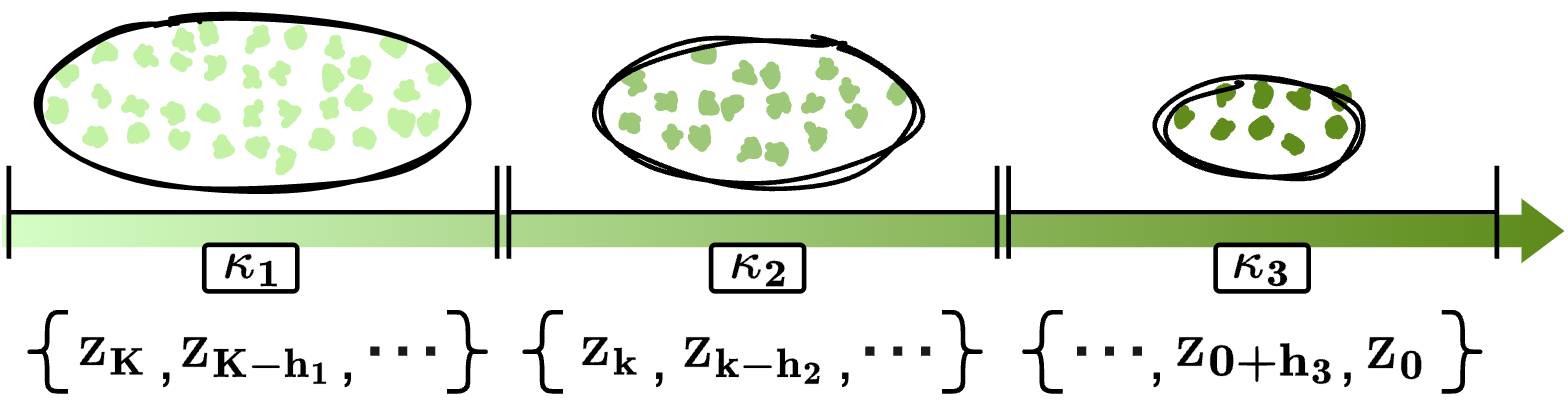
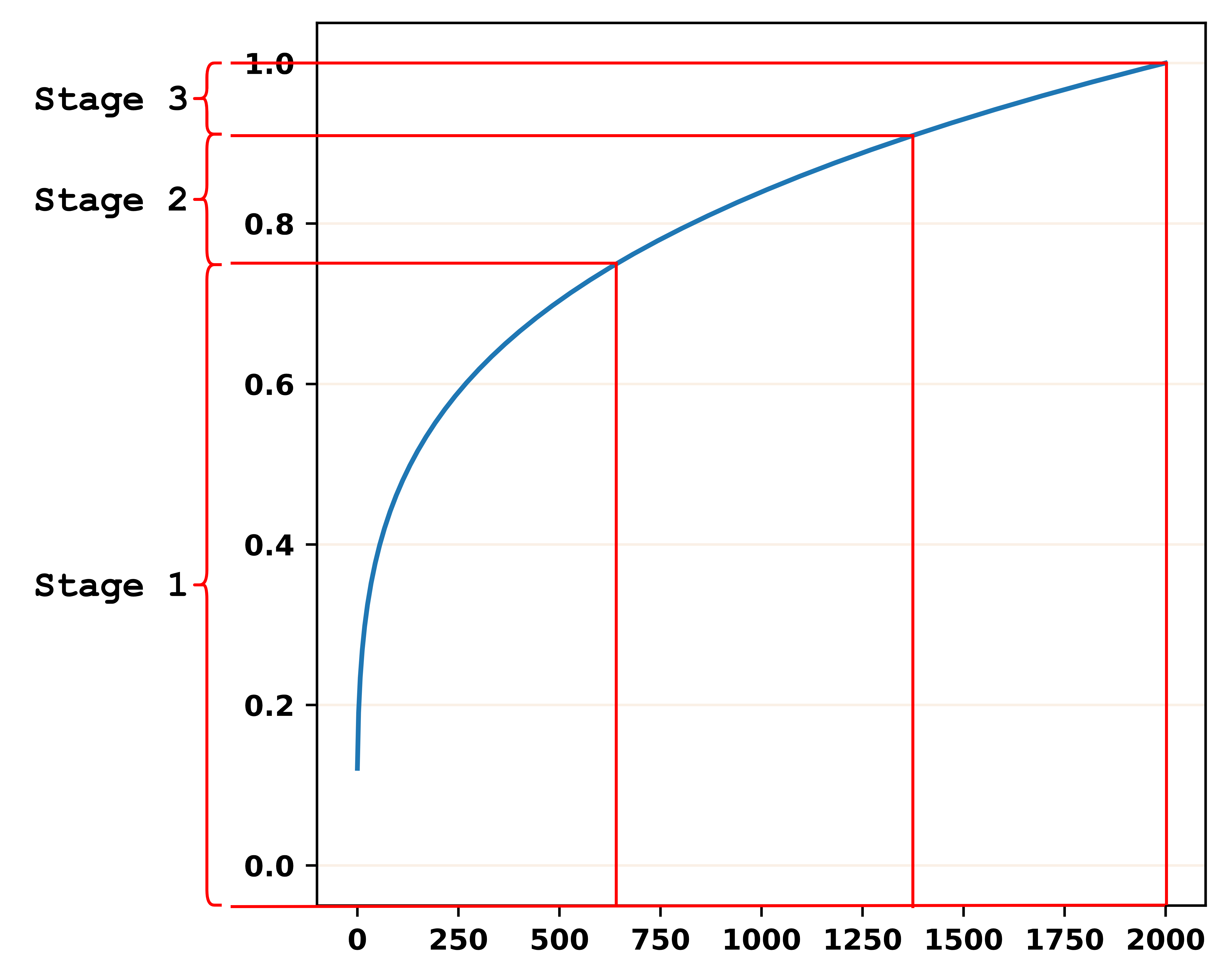
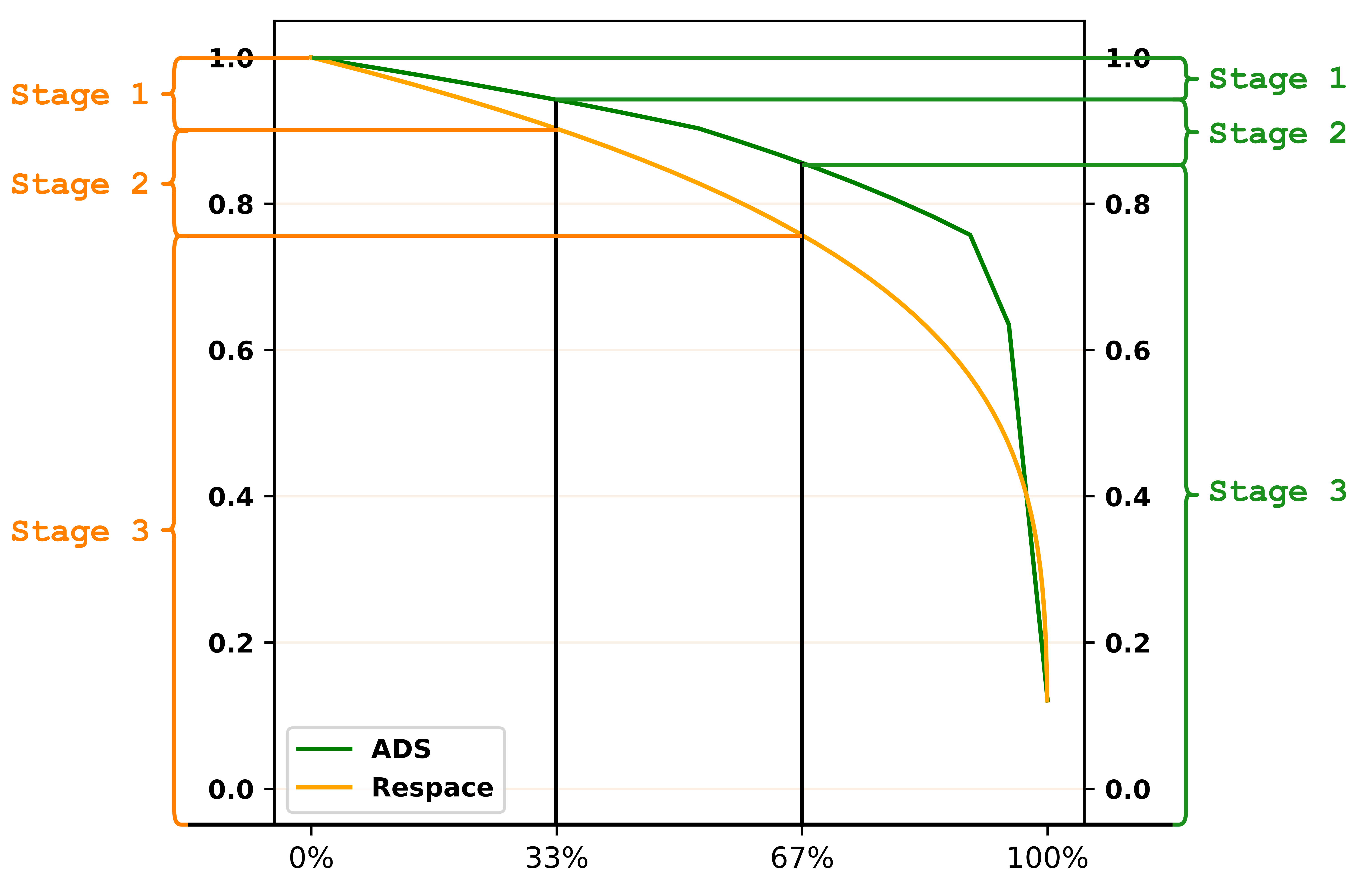
We also apply the Adaptive Decay Sampling (ADS) strategy to mitigate the issues brought by uniform downsampling. More concretely, we split the reverse process into three stages $[\kappa_{1},\kappa_{2},\kappa_{3}]$ and adaptively adjust the downsampled steps in each stage according to the total amount of added noise of each stage during the training, i.e., more downsampled steps are required to decompose the large noise, which is controlled by $\bar{\alpha}_{1:k}$ (Equation 3):

\eta_{i}=\left\{\begin{aligned} &\frac{1}{\sqrt{1-\bar{\alpha}_{Ki/3}}}-\sum\limits_{j=1}^{i-1}\eta_{j}&i>1&\\ &\frac{1}{\sqrt{1-\bar{\alpha}_{K/3}}}&i=1&\end{aligned}\right.

(10)

Then, we can treat $\eta_{i}$ as the weight to split the total downsampled steps $\mathcal{T}^{\prime}$ into different subsets for each stage $\kappa_{i}$ . Such a strategy is associated with the noise scheduler, which controls the calculation of $\bar{\alpha}_{1:k}$ , and we put more details in Appendix E.

5 Experiment

5.1 Settings

We describe the main settings of our experiments in this section, and more implementation details can be referred to Appendix C.

Tasks & Datasets

We conduct the experiments on three different generation tasks, i.e., directed, open-ended, and controllable. For directed generation tasks, we utilize the WIkI-AUTO corpus Jiang et al. (2020) for Text Simplification task and Quora Question Pairs⁶⁶6https://www.kaggle.com/c/quora-question-pairs corpus for Paraphrase task. For open-ended generation tasks, we adopt the ROC Stories (ROC) corpus for Story Generation task and Quasar-T Dhingra et al. (2017) dataset preprocessed by Lin et al. (2018) and Gong et al. (2022)⁷⁷7https://drive.google.com/drive/folders/122YK0IElSnGZbPMigXrduTVL1geB4wEW?usp=sharing for Question Generation task. For controllable text generation task, we utilize the E2E Novikova et al. (2017) dataset and select Semantic Content control task and Syntax Spans control task. More statistics of datasets are listed in Table 8 of Appendix C.1.

Baselines

We apply the DIFFSEQ Gong et al. (2022) as the baseline for directed generation tasks and open-ended generation tasks and utilize Diffusion-LM Li et al. (2022) for controllable generation tasks. For both of the above two baselines, we implement $f_{\theta}$ with Transformer model and select the converged checkpoint for post-training. The total diffusion steps $T$ for training and $K$ for post-training are both 2,000. We set the hyper-parameter $\gamma$ of $\mathcal{L}_{simple}^{dis}$ as 2 and utilize the square-root noise schedule for $\beta_{t}$ . Besides, we also compare the generation results with the autoregressive (AR) model BART Lewis et al. (2020) and the none-autoregressive (NAR) model CMLM Ghazvininejad et al. (2019), which are both implemented with the open library Fairseq toolkit⁸⁸8https://github.com/facebookresearch/fairseq Ott et al. (2019). For open-ended generation task, we utilize nucleus sampling Holtzman et al. (2019) (top- $p$ =0.5) for the BART model. Meanwhile, for the controllable generation tasks, we apply PPLM Dathathri et al. (2019) and FUDGE Yang and Klein (2021) for guidance.

Evaluation Metrics

For open-ended generation tasks, we report BLEU (B- $n$ ) Papineni et al. (2002), ROUGE (R-n) Lin (2004), Distinct (D- $n$ ) Li et al. (2016), Lexical Repetition (Rep- $n$ , 4-gram repetition for $n$ -times) Shao et al. (2019), BERTScore Zhang et al. (2019a), Mauve score (Mav) Pillutla et al. (2021), Perplexity (PPL), and Semantic Similarity (SIM, semantic similarity between generations and corresponding prompts) Guan et al. (2021)⁹⁹9https://huggingface.co/sentence-transformers/bert-base-nli-mean-tokens. We select part of the metrics mentioned above for the evaluation of directed generation tasks and utilize success rate (Ctrl) Li et al. (2022) to evaluate the control effect. The setting of $n$ is described in each subsection below, and the evaluation results (D- $n$ , Rep- $n$ , and PPL) of the golden text are reported for comparison. For fair comparison, we calculate the PPL and Mauve score with the same pre-trained GPT-2 Radford et al. model¹⁰¹⁰10https://huggingface.co/gpt2-large. We also fine-tune the GPT-2 model on each downstream dataset and report their PPL and Mauve score in Appendix F.1.

Data	Model	Step	B-2 $(\uparrow$ )	B-4 $(\uparrow$ )	R-2 $(\uparrow$ )	R-L $(\uparrow$ )	D-2 $(\uparrow$ )	LR-2 $(\downarrow$ )	BS $(\uparrow$ )	Mav $(\uparrow$ )	$\Delta$ PPL $(\downarrow$ )	SIM $(\downarrow$ )
ROC	CMLM	-	8.17	2.52	4.36	19.74	14.95	25.60	51.68	2.73	13.45 (+)	15.38
	BART	-	7.55	2.38	3.95	18.83	15.88	0.98	57.01	70.64	2.95 (-)	16.19
	DIFFSEQ $\dagger$	2,000	8.39	2.48	3.81	18.88	22.64	0.71	54.19	34.45	49.44 (+)	16.03
	+ Ours $\dagger$	2,000	8.90	2.66	4.27	19.59	19.86	1.22	54.91	41.56	33.56 (+)	15.94
	Respace $\ddagger$	20	8.43	2.48	3.83	18.87	22.93	0.75	53.80	25.37	56.32 (+)	16.06
	+ Ours $\ddagger$	20	8.86	2.63	4.16	19.58	21.48	0.90	54.05	28.06	48.76 (+)	15.96
	Golden	-	-	-	-	-	36.50	0.02	-	-	29.72	16.49
Quasar-T	CMLM	-	13.37	7.69	12.19	26.26	9.95	15.70	50.53	1.96	88.37 (+)	17.38
	BART	-	11.92	7.45	11.07	23.34	10.87	0.00	57.07	3.09	0.75 (+)	18.08
	DIFFSEQ $\dagger$	2,000	23.50	17.11	23.10	36.32	21.95	11.34	62.25	4.68	95.68 (+)	15.84
	+ Ours $\dagger$	2,000	23.67	17.53	23.34	36.55	19.75	12.07	62.80	10.91	58.68 (+)	15.87
	Respace $\ddagger$	20	23.15	16.92	22.75	35.97	25.20	10.31	61.76	4.53	169.75 (+)	15.80
	+ Ours $\ddagger$	20	23.55	17.45	23.17	36.02	21.18	11.23	62.52	5.41	96.83 (+)	15.85
	Golden	-	-	-	-	-	8.32	0.00	-	-	147.07	14.45

Table 1: Open-ended text generation results, where we also report the evaluation results of the ground truth (Golden).

5.2 Results

For all experiments, we compare the performance under the settings of full 2,000 reverse steps and uniformly downsampled 20 steps, aka Respace. We apply the Minimal Bayesian Risk method Li et al. (2022) and set candidate size $|\mathcal{S}|$ as 10.

Open-ended Text Generation

We report the open-ended generation results in Table 1 and observe that our method with 2,000 reverse steps can exceed the DIFFSEQ on most of the evaluation metrics (except for the Distinct and Lexical Repetition metrics), especially for PPL and Mauve scores that have significant improvement, which means our method can generate high-quality and fluency results. For downsampled 20 steps, we can find that our method still surpasses the Respace method except for the diversity metrics (D-2 and LR-2) and suffers from a smaller decrease when compared with DIFFUSEQ results of 2,000 steps. The reason for the high diversity of baselines is that the original DIFFSEQ model or Respace method can generate many meaningless texts, which leads to hard-to-read sentences (high PPL score). More details can be referred to Case Study in Appendix H. Besides, our method also achieves better performance than language models, i.e., CMLM and BART.

Directed Text Generation

Data	Model	B-2( $\uparrow$ )	B-4( $\uparrow$ )	R-2( $\uparrow$ )	R-L( $\uparrow$ )	$\Delta$ PPL( $\downarrow$ )
WIKI AUTO	CMLM	43.12	35.26	47.59	58.46	2.74 (-)
	BART	42.97	35.10	47.81	58.75	3.11 (-)
	DIFFSEQ $\dagger$	44.02	36.08	47.18	58.43	4.64 (+)
	+ Ours $\dagger$	45.26	37.33	48.35	59.82	2.04 (-)
	Respace $\ddagger$	42.13	33.97	45.33	57.05	17.44 (+)
	+ Ours $\ddagger$	44.61	36.51	47.61	58.81	3.29 (+)
QQP	CMLM	35.67	21.78	34.51	56.12	12.56 (+)
	BART	33.94	20.94	33.29	54.80	8.34 (+)
	DIFFSEQ $\dagger$	39.75	24.50	38.13	60.40	52.15 (+)
	+ Ours $\dagger$	41.74	26.27	40.56	61.88	28.01 (+)
	Respace $\ddagger$	38.58	23.67	36.67	59.11	90.61 (+)
	+ Ours $\ddagger$	41.43	25.81	39.88	61.62	35.57 (+)

Table 2: Directed text generation results, where

\dagger

denotes 2,000 steps, and

\ddagger

represents 20 steps.

Table 2 summarizes the directed text generation results. We can observe that the improvement in directed text generation tasks is significant that our method achieves better performance than both DIFFSEQ (2,000 steps) and Respace strategy (20 steps), especially the PPL score. We provide more evaluation results of directed generation tasks in Appendix F.2.

Controllable Text Generation

Data	Model	Ctrl ( $\uparrow$ )	PPL( $\downarrow$ )	LR-2 ( $\downarrow$ )
E2E (Semantic Content)	PPLM	21.03	6.04	4.18
	Diffusion-LM $\dagger$	81.46	2.52	0.08
	+ Ours $\dagger$	85.06	2.38	0.68
	Respace $\ddagger$	75.67	2.94	0.56
	+ Ours $\ddagger$	81.87	2.66	2.18
E2E (Syntax Spans)	FUDGE	54.20	4.03	-
	Diffusion-LM $\dagger$	91.12	2.52	0.35
	+ Ours $\dagger$	95.33	2.33	1.54
	Respace $\ddagger$	82.00	2.76	0.41
	+ Ours $\ddagger$	93.15	2.68	2.39

Table 3: Results of controllable text generation.

The results of controllable text generation are listed in Table 3, where we follow the official setting to evaluate the PPL¹¹¹¹11https://github.com/XiangLi1999/Diffusion-LM/blob/main/train_run.py. Our method can achieve a better control quality than baselines with higher Ctrl scores and generate more fluency results with lower PPL scores but suffers from low diversity.

5.3 Ablation Study

We conduct the ablation study on the ROC dataset and set candidate size $|\mathcal{S}|=1$ in this section.

Effect of Distance Penalty

We first explore the influence of Distance Penalty by adjusting the hyper-parameter $\omega$ and report the results in Table 4. We can observe that when the constraint becomes larger, i.e., $\omega$ from 1 to 6, the model can generate more fluent and precise texts but at the cost of diversity. Besides, we also find that our method can surpass the simple post-training strategy, i.e., $\omega=0$ , which means the improvement is brought by the Distance Penalty rather than post-training, which leads to over-fitting on the training data.

Effect of Downsampling Range

To explore the effect of downsampling range $\mathcal{R}_{k}$ in the training stage, we set the range with the constant and report the results in Table 5. We can observe that as the range becomes larger, i.e., more injected noises, the model can generate more fluent results (lower PPL) and more precise results (higher B-2 and R-2) with a smaller sampling range. Thus, adaptively adjusting the sampling range is essential for making a trade-off among different metrics.

$\gamma$	B-2( $\uparrow$ )	R-2 ( $\uparrow$ )	D-2( $\uparrow$ )	PPL( $\downarrow$ )	BS( $\uparrow$ )	SIM( $\downarrow$ )
0	8.23	3.69	25.51	99.33	52.94	16.08
1	8.38	3.77	23.40	94.53	53.70	16.02
2	8.67	3.99	21.01	88.44	53.68	15.99
4	8.81	4.11	17.29	81.06	53.17	15.95
6	8.85	4.15	17.35	82.87	53.07	15.96

Table 4: The influence of penalty weight

\gamma

Range	Steps	B-2( $\uparrow$ )	R-2 ( $\uparrow$ )	D-2( $\uparrow$ )	PPL( $\downarrow$ )	BS( $\uparrow$ )	SIM( $\downarrow$ )
400	2,000	8.26	3.75	21.92	75.10	54.71	16.07
400	20	8.27	3.68	23.43	89.09	54.10	16.06
200	2,000	8.36	3.85	21.45	75.51	54.65	16.05
200	20	8.36	3.76	23.45	93.71	53.88	16.00
100	2,000	8.50	3.92	21.16	73.60	54.69	16.03
100	20	8.38	3.77	23.40	94.53	53.70	16.02
10	2,000	8.50	3.93	20.98	74.05	54.70	16.05
10	20	8.42	3.84	24.24	101.62	53.60	16.06

Table 5: The influence of down-sampling range.

Comparison of Sampling Strategies

Steps	Strategy	B-2( $\uparrow$ )	R-2 ( $\uparrow$ )	D-2( $\uparrow$ )	LR-2 ( $\downarrow$ )	PPL( $\downarrow$ )
2,000	-	8.50	3.92	21.16	0.67	73.60
200 ( $\times 10$ )	Respace	8.50	3.89	20.97	0.69	73.64
	DDIM	8.47	3.86	17.65	1.51	77.56
	ADS	8.58	3.98	21.00	0.47	73.86
20 ( $\times 100$ )	Respace	8.53	3.86	20.92	0.59	79.08
	DDIM	7.61	3.79	15.00	3.55	73.77
	ADS	8.59	3.90	19.21	0.51	75.25
10 ( $\times 200$ )	Respace	8.45	3.73	21.80	0.67	90.01
	DDIM	6.98	3.46	14.64	4.87	77.81
	ADS	8.65	3.91	19.02	0.86	80.19
5 ( $\times 400$ )	Respace	7.87	3.27	30.55	0.55	192.43
	DDIM	6.56	3.20	14.30	6.75	88.05
	ADS	8.33	3.63	19.14	0.86	98.24

Table 6: Comparison of different sampling strategies. The number

\times n

in brackets illustrates the speedup ratio compared with 2,000 reverse steps.

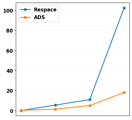
We compare our ADS method with the Respace and the DDIM strategies (Appendix E.3) and can observe that ADS can achieve a better performance (B-2 and R-2) and generate more fluency texts compared with Respace and more diverse texts compared with DDIM. Besides, the performance decline of ADS is smaller than the other two strategies, which shows the robustness of ADS (Appendix F.5).

Metrics	2000 steps				20 steps
Metrics	Win	Loss	Tie	$\zeta$	Win	Loss	Tie	$\zeta$
Fluency	20.6	13.8	65.6	85.9	31.1	15.0	53.9	66.6
Coherence	21.7	12.8	65.5	71.0	32.8	17.2	50.0	74.0
Relevance	27.8	16.1	56.1	87.8	26.7	15.6	57.7	81.7

Table 7: Human evaluation results on two different settings, where

\zeta

denotes Fleiss’ kappa value.

5.4 Human Evaluation

We compare our method with the vanilla diffusion model on six tasks under 2000 and 20 inference step settings for human evaluation. For each setting, we randomly sample 10 comparison pairs for every task and hire three annotators to give their preferences (win, loss, and tie) for three evaluation criteria: fluency, coherence, and relevance. More details can be referred to Appendix G. To ensure consistency among the three annotators, we report the Fleiss’ kappa score Fleiss (1971). The results are shown in Table 7, and we can observe that all the inter-annotator agreements are substantially consistent ( $\zeta\in[0.6,1]$ ) and our method can achieve better performance than the vanilla diffusion model under both settings. More concretely, as the number of reverse steps decreases, our method can drive the model to generate much better results than the vanilla diffusion model.

6 Related Work

6.1 Text Generation via Diffusion Model

Denoising diffusion probabilistic models Ho et al. (2020) have shown promising performance on text generation tasks Yang et al. (2022); Li et al. (2022); Gong et al. (2022); Austin et al. (2021). There exist two main methodologies, including modeling on discrete state spaces or continuous state spaces Sohl-Dickstein et al. (2015). Early works mainly focus on designing one discrete corrupting process on discrete space by introducing the absorbing tokens Austin et al. (2021) or transforming the intermediate state into a uniform categorical base distribution Hoogeboom et al. (2021). However, such discrete modeling suffers from the scaling of one-hot vectors Gong et al. (2022), which can be only qualified for uncontrollable text generation. Li et al. (2022) propose the Diffusion-LM, which models the data in the continuous space with one mapping function connecting the continuous space and discrete text space. Gong et al. (2022); Han et al. (2022) combine the diffusion model with iterative NAR model Gu et al. (2019) and semi-AR model Wang et al. (2018) to further improve the performance in text generation tasks. Nevertheless, the approaches above all suffer the inefficiency of inference (reverse process), and the quality of generated text decreases remarkably when applying less denoising steps He et al. (2022).

6.2 Inference Acceleration of Diffusion Model

One critical drawback of Diffusion Models is that they require many iterations to produce high-quality results. Song et al. (2020) propose one denoising diffusion implicit model (DDIM) and redefine the sampling function to accelerate the generation process. Jolicoeur-Martineau et al. (2021) devise a faster SDE solver for reverse diffusion processes, and Salimans and Ho (2021) distill a trained deterministic diffusion sampler into a new diffusion model, which only takes half of the sampling steps to generate a full image. Recent work Kim and Ye (2022) also proposes an orthogonal approach Denoising MCMC to accelerate the score-based sampling process of the diffusion model. Nevertheless, all the methods above are designed for the computer vision field, and the inference acceleration of diffusion for text generation is still unexplored.

6.3 Exposure Bias of Autoregressive Model

Exposure Bias is widely recognized as a central challenge in autoregressive models, primarily due to the discrepancies between training and test-time generation, which can result in incremental distortion during the testing phase Bengio et al. (2015); Schmidt (2019); He et al. (2021). To mitigate such issue, three mainstream methods have been adopted, including designing new training objectives Ranzato et al. (2015); Shen et al. (2016); Wiseman and Rush (2016); Zhang et al. (2019b), adding regularization terms to standard training objective function Zhang et al. (2019c), as well as adopting reinforcement learning approaches Bahdanau et al. (2016); Brakel et al. (2017) to minimize the expected loss with Minimum Risk Training.

7 Conclusion

This work focuses on bridging the training and inference gaps of the diffusion model. The result of the preliminary study shows that injecting predicted noise into the model can help mitigate the gaps, and the uniform downsampling strategy for inference acceleration harms the model performance. Thus, we propose two simple yet effective strategies: Distance Penalty and Adaptive Decay Sampling, to mitigate the aforementioned gaps. Experiments on 6 text generation tasks of 3 different settings show that the model with our methods can achieve better performance and great inference speedup.

8 Limitation

Although our method can improve the performance as well as accelerate the inference speed, it suffers from two problems: (1) the diversity of generated results is low compared with language models (LMs) due to the clamp sampling strategy, and (2) the diffusion steps of post-tuning stage should stay consistent with the steps in the training stage, and there still exists the gaps between training and inference, i.e., $|\mathcal{T}|=|\mathcal{K}|\neq|\mathcal{T}^{\prime}|$ , To mitigate the aforementioned two issues, we can explore a better post-training or training strategy to mitigate the training-inference gaps further. In addition, we found that the diffusion model does not perform well in open-ended generation tasks, such as generating incoherent sentences. This is closely related to the drawbacks of NAR models, which have a strong conditional independence assumption. We will attempt to address this issue in the future.

Ethics Statement

It is worth noting that all the data used in this paper are publicly available, and we utilize the same evaluation scripts to make sure that all the comparisons are fair. We have replaced the people names in the corpora with special placeholders to mitigate the problematic biases Radford et al. issue of generation results. Although we have taken some methods to mitigate the problematic biases, such a problem cannot be solved completely. We urge the users to cautiously apply our methods in the real world and carefully check the generation results.

Acknowledgement

This work is supported by the National Science Foundation of China (NSFC No. 62206194 and No. 62106165), the Natural Science Foundation of Jiangsu Province, China (Grant No. BK20220488), and the Project Funded by the Priority Academic Program Development of Jiangsu Higher Education Institutions. This work is also supported by Beijing Academy of Artificial Intelligence (BAAI).

References

Austin et al. (2021) Jacob Austin, Daniel D Johnson, Jonathan Ho, Daniel Tarlow, and Rianne van den Berg. 2021. Structured denoising diffusion models in discrete state-spaces. Advances in Neural Information Processing Systems, 34:17981–17993.
Bahdanau et al. (2016) Dzmitry Bahdanau, Philemon Brakel, Kelvin Xu, Anirudh Goyal, Ryan Lowe, Joelle Pineau, Aaron Courville, and Yoshua Bengio. 2016. An actor-critic algorithm for sequence prediction. arXiv preprint arXiv:1607.07086.
Bengio et al. (2015) Samy Bengio, Oriol Vinyals, Navdeep Jaitly, and Noam Shazeer. 2015. Scheduled sampling for sequence prediction with recurrent neural networks. Advances in neural information processing systems, 28.
Brakel et al. (2017) Dzmitry Bahdanau Philemon Brakel, Kelvin Xu Anirudh Goyal, RL PINEAU, Aaron Courville, and Yoshua Bengio. 2017. An actor-critic algorithm for sequence prediction. In Open Review. net. International Conference on Learning Representations, pages 1–17.
Dathathri et al. (2019) Sumanth Dathathri, Andrea Madotto, Janice Lan, Jane Hung, Eric Frank, Piero Molino, Jason Yosinski, and Rosanne Liu. 2019. Plug and play language models: A simple approach to controlled text generation. In International Conference on Learning Representations.
Dhingra et al. (2017) Bhuwan Dhingra, Kathryn Mazaitis, and William W Cohen. 2017. Quasar: Datasets for question answering by search and reading. arXiv preprint arXiv:1707.03904.
Fleiss (1971) Joseph L Fleiss. 1971. Measuring nominal scale agreement among many raters. Psychological bulletin, 76(5):378.
Gao et al. (2022) Zhujin Gao, Junliang Guo, Xu Tan, Yongxin Zhu, Fang Zhang, Jiang Bian, and Linli Xu. 2022. Difformer: Empowering diffusion model on embedding space for text generation. arXiv preprint arXiv:2212.09412.
Ghazvininejad et al. (2019) Marjan Ghazvininejad, Omer Levy, Yinhan Liu, and Luke Zettlemoyer. 2019. Mask-predict: Parallel decoding of conditional masked language models. In Proceedings of the 2019 Conference on Empirical Methods in Natural Language Processing and the 9th International Joint Conference on Natural Language Processing (EMNLP-IJCNLP), pages 6112–6121.
Gong et al. (2022) Shansan Gong, Mukai Li, Jiangtao Feng, Zhiyong Wu, and LingPeng Kong. 2022. Diffuseq: Sequence to sequence text generation with diffusion models. arXiv preprint arXiv:2210.08933.
Goodfellow et al. (2020) Ian Goodfellow, Jean Pouget-Abadie, Mehdi Mirza, Bing Xu, David Warde-Farley, Sherjil Ozair, Aaron Courville, and Yoshua Bengio. 2020. Generative adversarial networks. Communications of the ACM, 63(11):139–144.
Gu et al. (2019) Jiatao Gu, Changhan Wang, and Junbo Zhao. 2019. Levenshtein transformer. Advances in Neural Information Processing Systems, 32.
Guan et al. (2021) Jian Guan, Xiaoxi Mao, Changjie Fan, Zitao Liu, Wenbiao Ding, and Minlie Huang. 2021. Long text generation by modeling sentence-level and discourse-level coherence. In Proceedings of the 59th Annual Meeting of the Association for Computational Linguistics and the 11th International Joint Conference on Natural Language Processing (Volume 1: Long Papers), pages 6379–6393.
Han et al. (2022) Xiaochuang Han, Sachin Kumar, and Yulia Tsvetkov. 2022. Ssd-lm: Semi-autoregressive simplex-based diffusion language model for text generation and modular control. arXiv preprint arXiv:2210.17432.
He et al. (2021) Tianxing He, Jingzhao Zhang, Zhiming Zhou, and James Glass. 2021. Exposure bias versus self-recovery: Are distortions really incremental for autoregressive text generation? In Proceedings of the 2021 Conference on Empirical Methods in Natural Language Processing, pages 5087–5102.
He et al. (2022) Zhengfu He, Tianxiang Sun, Kuanning Wang, Xuanjing Huang, and Xipeng Qiu. 2022. Diffusionbert: Improving generative masked language models with diffusion models. arXiv preprint arXiv:2211.15029.
Ho et al. (2020) Jonathan Ho, Ajay Jain, and Pieter Abbeel. 2020. Denoising diffusion probabilistic models. Advances in Neural Information Processing Systems, 33:6840–6851.
Holtzman et al. (2019) Ari Holtzman, Jan Buys, Li Du, Maxwell Forbes, and Yejin Choi. 2019. The curious case of neural text degeneration. In International Conference on Learning Representations.
Hoogeboom et al. (2021) Emiel Hoogeboom, Didrik Nielsen, Priyank Jaini, Patrick Forré, and Max Welling. 2021. Argmax flows and multinomial diffusion: Learning categorical distributions. Advances in Neural Information Processing Systems, 34:12454–12465.
Hoogeboom et al. (2022) Emiel Hoogeboom, Vıctor Garcia Satorras, Clément Vignac, and Max Welling. 2022. Equivariant diffusion for molecule generation in 3d. In International Conference on Machine Learning, pages 8867–8887. PMLR.
Huszár (2015) Ferenc Huszár. 2015. How (not) to train your generative model: Scheduled sampling, likelihood, adversary? arXiv preprint arXiv:1511.05101.
Jiang et al. (2020) Chao Jiang, Mounica Maddela, Wuwei Lan, Yang Zhong, and Wei Xu. 2020. Neural crf model for sentence alignment in text simplification. In Proceedings of the 58th Annual Meeting of the Association for Computational Linguistics, pages 7943–7960.
Jolicoeur-Martineau et al. (2021) Alexia Jolicoeur-Martineau, Ke Li, Rémi Piché-Taillefer, Tal Kachman, and Ioannis Mitliagkas. 2021. Gotta go fast when generating data with score-based models. arXiv preprint arXiv:2105.14080.
Kim and Ye (2022) Beomsu Kim and Jong Chul Ye. 2022. Denoising mcmc for accelerating diffusion-based generative models. arXiv preprint arXiv:2209.14593.
Kingma and Welling (2013) Diederik P Kingma and Max Welling. 2013. Auto-encoding variational bayes. arXiv preprint arXiv:1312.6114.
Kong et al. (2020) Zhifeng Kong, Wei Ping, Jiaji Huang, Kexin Zhao, and Bryan Catanzaro. 2020. Diffwave: A versatile diffusion model for audio synthesis. In International Conference on Learning Representations.
Lewis et al. (2020) Mike Lewis, Yinhan Liu, Naman Goyal, Marjan Ghazvininejad, Abdelrahman Mohamed, Omer Levy, Veselin Stoyanov, and Luke Zettlemoyer. 2020. Bart: Denoising sequence-to-sequence pre-training for natural language generation, translation, and comprehension. In Proceedings of the 58th Annual Meeting of the Association for Computational Linguistics, pages 7871–7880.
Li et al. (2016) Jiwei Li, Michel Galley, Chris Brockett, Jianfeng Gao, and William B Dolan. 2016. A diversity-promoting objective function for neural conversation models. In Proceedings of the 2016 Conference of the North American Chapter of the Association for Computational Linguistics: Human Language Technologies, pages 110–119.
Li et al. (2022) Xiang Lisa Li, John Thickstun, Ishaan Gulrajani, Percy Liang, and Tatsunori B Hashimoto. 2022. Diffusion-lm improves controllable text generation. arXiv preprint arXiv:2205.14217.
Lin (2004) Chin-Yew Lin. 2004. Rouge: A package for automatic evaluation of summaries. In Text summarization branches out, pages 74–81.
Lin et al. (2018) Yankai Lin, Haozhe Ji, Zhiyuan Liu, and Maosong Sun. 2018. Denoising distantly supervised open-domain question answering. In Proceedings of the 56th Annual Meeting of the Association for Computational Linguistics (Volume 1: Long Papers), pages 1736–1745.
Lin et al. (2022) Zhenghao Lin, Yeyun Gong, Yelong Shen, Tong Wu, Zhihao Fan, Chen Lin, Weizhu Chen, and Nan Duan. 2022. Genie: Large scale pre-training for text generation with diffusion model. arXiv preprint arXiv:2212.11685.
Mostafazadeh et al. (2016) Nasrin Mostafazadeh, Nathanael Chambers, Xiaodong He, Devi Parikh, Dhruv Batra, Lucy Vanderwende, Pushmeet Kohli, and James Allen. 2016. A corpus and cloze evaluation for deeper understanding of commonsense stories. In Proceedings of the 2016 Conference of the North American Chapter of the Association for Computational Linguistics: Human Language Technologies, pages 839–849.
Nichol and Dhariwal (2021) Alexander Quinn Nichol and Prafulla Dhariwal. 2021. Improved denoising diffusion probabilistic models. In International Conference on Machine Learning, pages 8162–8171. PMLR.
Novikova et al. (2017) Jekaterina Novikova, Ondřej Dušek, and Verena Rieser. 2017. The e2e dataset: New challenges for end-to-end generation. arXiv preprint arXiv:1706.09254.
Ott et al. (2019) Myle Ott, Sergey Edunov, Alexei Baevski, Angela Fan, Sam Gross, Nathan Ng, David Grangier, and Michael Auli. 2019. fairseq: A fast, extensible toolkit for sequence modeling. In Proceedings of the 2019 Conference of the North American Chapter of the Association for Computational Linguistics (Demonstrations), pages 48–53.
Papineni et al. (2002) Kishore Papineni, Salim Roukos, Todd Ward, and Wei-Jing Zhu. 2002. Bleu: a method for automatic evaluation of machine translation. In Proceedings of the 40th annual meeting of the Association for Computational Linguistics, pages 311–318.
Pillutla et al. (2021) Krishna Pillutla, Swabha Swayamdipta, Rowan Zellers, John Thickstun, Sean Welleck, Yejin Choi, and Zaid Harchaoui. 2021. Mauve: Measuring the gap between neural text and human text using divergence frontiers. Advances in Neural Information Processing Systems, 34:4816–4828.
(39) Alec Radford, Jeffrey Wu, Rewon Child, David Luan, Dario Amodei, Ilya Sutskever, et al. Language models are unsupervised multitask learners.
Ramesh et al. (2022) Aditya Ramesh, Prafulla Dhariwal, Alex Nichol, Casey Chu, and Mark Chen. 2022. Hierarchical text-conditional image generation with clip latents. arXiv preprint arXiv:2204.06125.
Ranzato et al. (2015) Marc’Aurelio Ranzato, Sumit Chopra, Michael Auli, and Wojciech Zaremba. 2015. Sequence level training with recurrent neural networks. arXiv preprint arXiv:1511.06732.
Rombach et al. (2022) Robin Rombach, Andreas Blattmann, Dominik Lorenz, Patrick Esser, and Björn Ommer. 2022. High-resolution image synthesis with latent diffusion models. In Proceedings of the IEEE/CVF Conference on Computer Vision and Pattern Recognition, pages 10684–10695.
Salimans and Ho (2021) Tim Salimans and Jonathan Ho. 2021. Progressive distillation for fast sampling of diffusion models. In International Conference on Learning Representations.
Schmidt (2019) Florian Schmidt. 2019. Generalization in generation: A closer look at exposure bias. EMNLP-IJCNLP 2019, page 157.
Shao et al. (2019) Zhihong Shao, Minlie Huang, Jiangtao Wen, Wenfei Xu, and Xiaoyan Zhu. 2019. Long and diverse text generation with planning-based hierarchical variational model. In Proceedings of the 2019 Conference on Empirical Methods in Natural Language Processing and the 9th International Joint Conference on Natural Language Processing (EMNLP-IJCNLP), pages 3257–3268.
Shen et al. (2016) Shiqi Shen, Yong Cheng, Zhongjun He, Wei He, Hua Wu, Maosong Sun, and Yang Liu. 2016. Minimum risk training for neural machine translation. In Proceedings of the 54th Annual Meeting of the Association for Computational Linguistics (Volume 1: Long Papers), pages 1683–1692.
Sohl-Dickstein et al. (2015) Jascha Sohl-Dickstein, Eric Weiss, Niru Maheswaranathan, and Surya Ganguli. 2015. Deep unsupervised learning using nonequilibrium thermodynamics. In International Conference on Machine Learning, pages 2256–2265. PMLR.
Song et al. (2020) Jiaming Song, Chenlin Meng, and Stefano Ermon. 2020. Denoising diffusion implicit models. In International Conference on Learning Representations.
Strudel et al. (2022) Robin Strudel, Corentin Tallec, Florent Altché, Yilun Du, Yaroslav Ganin, Arthur Mensch, Will Grathwohl, Nikolay Savinov, Sander Dieleman, Laurent Sifre, et al. 2022. Self-conditioned embedding diffusion for text generation. arXiv preprint arXiv:2211.04236.
Vaswani et al. (2017) Ashish Vaswani, Noam Shazeer, Niki Parmar, Jakob Uszkoreit, Llion Jones, Aidan N Gomez, Łukasz Kaiser, and Illia Polosukhin. 2017. Attention is all you need. Advances in neural information processing systems, 30.
Wang et al. (2018) Chunqi Wang, Ji Zhang, and Haiqing Chen. 2018. Semi-autoregressive neural machine translation. In Proceedings of the 2018 Conference on Empirical Methods in Natural Language Processing, pages 479–488.
Wiseman and Rush (2016) Sam Wiseman and Alexander M Rush. 2016. Sequence-to-sequence learning as beam-search optimization. arXiv preprint arXiv:1606.02960.
Yang and Klein (2021) Kevin Yang and Dan Klein. 2021. Fudge: Controlled text generation with future discriminators. In Proceedings of the 2021 Conference of the North American Chapter of the Association for Computational Linguistics: Human Language Technologies, pages 3511–3535.
Yang et al. (2022) Ling Yang, Zhilong Zhang, Yang Song, Shenda Hong, Runsheng Xu, Yue Zhao, Yingxia Shao, Wentao Zhang, Bin Cui, and Ming-Hsuan Yang. 2022. Diffusion models: A comprehensive survey of methods and applications. arXiv preprint arXiv:2209.00796.
Zhang et al. (2019a) Tianyi Zhang, Varsha Kishore, Felix Wu, Kilian Q Weinberger, and Yoav Artzi. 2019a. Bertscore: Evaluating text generation with bert. In International Conference on Learning Representations.
Zhang et al. (2019b) Wen Zhang, Yang Feng, Fandong Meng, Di You, and Qun Liu. 2019b. Bridging the gap between training and inference for neural machine translation. In Proceedings of the 57th Annual Meeting of the Association for Computational Linguistics, pages 4334–4343.
Zhang et al. (2019c) Zhirui Zhang, Shuangzhi Wu, Shujie Liu, Mu Li, Ming Zhou, and Tong Xu. 2019c. Regularizing neural machine translation by target-bidirectional agreement. In Proceedings of the AAAI Conference on Artificial Intelligence, volume 33, pages 443–450.

Appendix A Preliminary of Diffusion Model

In this section, we provide more details of training and inference.

Training Objective

The training objective of the diffusion model is to maximize the marginal likelihood of distribution $\mathbb{E}_{z_{0}\sim p_{data}}\left[\log p_{\theta}(z_{0})\right]$ , and the variational lower bound (VLB) can be written as:

		$\displaystyle\mathcal{L}_{vlb}=\mathop{\mathbb{E}}\limits_{q(z_{1:T}\mid z_{0})}[\log\frac{q(z_{T}\mid z_{0})}{p_{\theta}(z_{T})}$		(11)
		$\displaystyle+\sum\limits_{t=2}^{T}\log\frac{q(z_{t-1}\mid z_{0},z_{t})}{p_{\theta}(z_{t-1}\mid z_{t})}-\log p_{\theta}(z_{0}\mid z_{1})]$		(11)

Training

During the training stage, each intermediate noise $z_{t-1}~{}(1\leq t\leq T+1)$ of the forward process can be obtained directly by accumulative multiplication with Equation 1:

q(z_{t}\mid z_{0})=\mathcal{N}(z_{t};\sqrt{\bar{\alpha}_{t}}z_{0},(1-\bar{\alpha}_{t})\mathrm{I}),

(12)

where $\alpha_{t}=1-\beta_{t}$ and $\bar{\alpha}_{t}=\prod_{i=1}^{t}\alpha_{i}$ .

It is worth noting that, according to the reparameterization method, the value of $1-\bar{\alpha}_{t}$ denotes the variance of accumulated noise of the current step $z_{t-1}$ , i.e., controlling how much noise should be added at the current step.

Combined with Equation 3, Equation 4 and Equation 12, the training process can be referred to Algorithm 1 Ho et al. (2020).

Algorithm 1 Training Process

1:repeat

2: sample

z_{0}\sim q(z_{0})

3: sample

t\sim\mathrm{Uniform}(\{1,\cdots,T\})

4: sample

\epsilon\sim\mathcal{N}(0,\mathrm{I})

5: calculate

z_{t}=\sqrt{\bar{\alpha}_{t}}z_{0}+\sqrt{1-\bar{\alpha}_{t}}\epsilon

6: gradient descent on

\nabla_{\theta}||\epsilon-\epsilon_{\theta}(z_{t},t)||^{2}

7:until converged

Inference

For the inference stage, there only exists the reverse process, and each intermediate state $z_{t-1}$ is strictly conditioned on the previous history. It can be summarized into Algorithm 2:

Algorithm 2 Inference Process

1:sample

z_{T}\sim\mathcal{N}(0,\mathrm{I})

2:for

t\leftarrow T,\cdots,1

3: sample

\epsilon\sim\mathcal{N}(0,\mathrm{I})

t>1

,else

\epsilon=0

z_{t-1}=\frac{1}{\sqrt{\alpha_{t}}}(z_{t}-\frac{\beta_{t}}{\sqrt{1-\bar{\alpha}_{t}}}\epsilon_{\theta}(z_{t},t))+\theta_{t}\epsilon

5:end for

6:return

z_{0}

Appendix B Diffusion Models for Text Generation

In this section, we provide more details about Embedding Setting, Clamping Strategy, and Partially Noising Strategy.

Embedding Setting

As mentioned in Section 2.2, given the embedding function $\mathcal{E}(\cdot)$ , we can map the discrete text into the continuous space or transform the noise back to the discrete text. Specifically, such mapping strategy, also called rounding Li et al. (2022), is achieved by selecting the most probable word in the embedding space by argmax operation: $p_{\theta}(\mathrm{w}\mid z_{0})=\prod_{i=1}^{L}p_{\theta}(w_{i}\mid z_{0}^{i})$ , where $p_{\theta}(w_{i}\mid z_{0}^{i})$ is a softmax distribution and $z_{0}^{i}$ denotes the $i$ -th position of $z_{0}$ distribution. To train the embedding $\mathcal{E}$ , the simplified training objective (Equation 4) should be rewritten as:

	$\displaystyle\mathcal{L}^{\prime}_{simple}=$	$\displaystyle\mathcal{L}_{simple}+\sum\limits_{t=1}^{T}\mathop{\mathbb{E}}\limits_{q(z_{0:T}\mid\mathrm{w})}[\|\|\mathcal{E}(\mathrm{w})-$		(13)
		$\displaystyle\mu_{\theta}(z_{1},1)\|\|^{2}+\log p_{\theta}(\mathrm{w}\mid z_{0})]$		(13)

Clamping Strategy

To make the rounding operation more precise, the diffusion model applies the Clamping strategy Li et al. (2022), which forces each predicted vector to commit to its nearest word vector through the embedding $\mathcal{E}$ in each reverse step during the inference. Thus, combined with Equation 3, the sampling function of Equation 5 should be rewritten as:

z_{t-1}=\sqrt{\overline{\alpha}}\mathrm{Clamp}(f_{\theta}(z_{t},t))+\sqrt{1-\overline{\alpha}}\epsilon

(14)

Besides, it also approximate the training objective of Equation 13 into Equation 15 by scaling the constants:

		$\displaystyle\mathcal{L}_{simple}^{text}=\mathop{\mathbb{E}}\limits_{q(z_{0:T}\mid\mathrm{w})}\Big{[}\|\|\hat{\mu}({z_{T};z_{0}}\|\|^{2}+\sum\limits^{T}_{t=2}\|\|\hat{\mu}(z_{t};z_{0})$		(15)
		$\displaystyle-\mu_{\theta}(z_{t},t)\|\|^{2}\Big{]}+\mathop{\mathbb{E}}\limits_{q(z_{0:1}\mid\mathrm{w})}\big{[}\|\|\mathcal{E}(\mathrm{w})-f_{\theta}(z_{1},1)\|\|^{2}$
		$\displaystyle-\log p_{\theta}(\mathrm{w}\mid z_{0})\big{]},$

where each reverse diffusion step estimates the $z_{0}$ directly rather than $\hat{\mu}({z_{t},z_{0}})$ .

Partially Noising Strategy

For sequence-to-sequence text generation tasks, Gong et al. (2022) propose the Partially Noising Strategy that simply perturbs the target text $\mathbf{w}^{x}$ and recovers it conditioned on the source text $\mathbf{w}^{x}$ . More concretely, we concatenate $\mathbf{w}^{x}$ and $\mathbf{w}^{y}$ , denoted as $\mathbf{w}^{x\bigoplus y}$ and utilize an anchor vector,i.e., $\mathcal{E}(\mathbf{w}^{x})$ , to replace the $\mathbf{w}^{x}$ part after each perturbance during the forward diffusion process. Then, the training objective of the diffusion model can be rewritten as:

	$\displaystyle\mathcal{L}_{seq}=$	$\displaystyle\mathcal{L}_{simple}+\sum\limits_{t=1}^{T}\mathop{\mathbb{E}}\limits_{q(z_{0:T}\mid\mathrm{w})}[\|\|\mathcal{E}(\mathrm{w}^{x\bigoplus y})-$		(16)
		$\displaystyle\mu_{\theta}(z_{1},1)\|\|^{2}+\log p_{\theta}(\mathrm{w}^{x\bigoplus y}\mid z_{0})]$		(16)

Appendix C Implementation Details

This section provides more details on dataset processing, baseline settings, and evaluation metrics.

C.1 Dataset Processing

We provide the statistics of each corpus in Table 8. For the ROC dataset, we mask all the names with special placeholders Guan et al. (2021) and only keep 4 sentences in the target. For directed and open-ended generation tasks, we apply the pre-trained tokenizer¹²¹²12https://huggingface.co/bert-base-uncased. For the E2E dataset, we apply the NLTK package¹³¹³13https://www.nltk.org/ for tokenization.

Data	#Train	#Valid	#Test
WIKI-AUTO	677,751	2,038	4,972
QQP	114,715	878	1,091
ROC Story	88,344	4,908	4,909
Quasar-T	116,953	2,048	10,000
E2E(Semantic)	333,123	-	3,365
E2E(Syntax)	41,640	-	421

Table 8: Statistics of datasets used in our experiments.

C.2 Baselines

We utilize Diffusion-LM Li et al. (2022) and DIFFSEQ Gong et al. (2022) as the diffusion model baselines, both of which are implemented with transformer model, which contains 12 layers and 12 attention heads. For a fair comparison, we utilize the language models CMLM Ghazvininejad et al. (2019) and BART Lewis et al. (2020) that have the same model architecture, i.e., Transformer-based model, and the number of model parameters. For the CMLM model, we set the iteration steps in inference as 10. The maximum sequence length is 64 for controllable generation and 128 for directed and open-ended generation tasks. All the models are trained from scratch, and we set total step $T=2000$ of the diffusion model and apply a square-root noise schedule $\bar{\alpha}_{t}=\sqrt{1-t/T+s}$ , where $s$ is a small constant. We conduct the experiments on 4 NVIDIA A100 (40GB) GPUs (directed generation and open-ended generation) and 1 NVIDIA TITAN V GPU (controllable generation¹⁴¹⁴14Due to the limitation of the platform.). We select the best checkpoint according to the loss on the validation set (directed generation and open-ended generation) or test the PPL value at the end of each epoch (controllable generation). The total training steps and training time (second) are listed in Table 9. To stay consistent with the baselines, we use the Minimum Bayesian Risk decoding (MBR) method Li et al. (2022) in all the experiments, setting the candidate size $|S|=10$ .

Data	Training Step	Time(s)
WIKI-AUTO	120,000	35,978
QQP	200,000	59,835
ROC	120,000	35,991
Quasar-T	200,000	59,911
E2E(Semantic)^∗	120,000	15,074
E2E(Syntax)^∗	120,000	15,074

Table 9: Statistics of training stage, where the datasets denoted with

*

share the same checkpoint.

C.3 Evaluation Metrics

For Lexical Repetition (LR- $n$ ) score, we calculate the repetition times $n$ of $k$ -gram texts in the generation results and select the hyper-parameter $n$ and $k$ according to the average generation length. Specifically, we choose $k=4,n=2$ for open-ended generation task, $k=2,n=2$ for directed generation task, and $k=2,n=1$ for controllable generation task. Besides, for the Semantic Similarity metric, we utilize the Sentence-BERT model¹⁵¹⁵15https://huggingface.co/sentence-transformers/bert-base-nli-mean-tokens to compress the whole sentence into a vector and utilize cosine similarity to calculate the distance between two vectors. We apply the pre-trained GPT-2 model¹⁶¹⁶16https://huggingface.co/gpt2-large to calculate the PPL score for open-ended and directed generation tasks as well as utilize the fine-tuned GPT-2 model with E2E dataset for controllable generation task.

Appendix D Gaps between Training and Inference

We provide more detailed preliminary experimental results in this section.

D.1 Training with Predicted Noise

In this section, we provide more details of noise replacement operation. If we want to replace the conditioned noise $z_{t+1}$ in $p_{\theta}(z_{t}\mid z_{t+1})$ with another noise $z_{t+\delta}$ , we can utilize Equation 2 which transform the probability distribution into the Gaussian distribution, and replace $\mu_{\theta}(z_{t+1},t+1)$ in Equation 2 with $\mu_{\theta}(z_{t+\delta},t+\delta)$ . More experimental results of noise injection are shown in Figure 6.

D.2 Extensive Trials

This section shows more results of the distance between the predicted reverse noise with the forward noise. We plot the result of models trained with 40K, 80K, and 120K steps and show the results of the randomly initialized model, i.e., trained with 0 step, in Figure 7. We can observe that the results of the trained models share a similar trend with Figure 4, which indicates that we can inject the predicted reverse noise in the early stage of training (Appendix F.4).

Appendix E Adaptive Decay Sampling

In this section, we introduce the concept of noise scheduler and explain the correlation between the Adaptive Decay Sampling (ADS) strategy and noise scheduler to help better understand our method. Besides we also describe the implementation details of the DDIM method. The overview of the Adaptive Sparse Sampling strategy is shown in Figure 8, where we split the total down-sampled steps into different subsets for three denoising stages $[\kappa_{1},\kappa_{2},\kappa_{3}]$ with weight $\eta_{i}(i\in\{1,2,3\})$

E.1 Noise Scheduler

The noise scheduler controls the amount of noise added to each diffusion forward step parameterized by $\bar{\alpha}_{1:T}$ . As shown in Figure 9, we plot the sqrt noise scheduler Li et al. (2022), which is defined by $\bar{\alpha}_{t}=1-\sqrt{t/T+s}$ , where $s=1e-4$ is a small constant that simulates the start noise. We can observe that the noise increases rapidly for the first 500 forward steps and slows down in the latter steps. When we split the total forward diffusion steps into three stages, we can find the model is trained to solve the high-noise with more steps during the training stage.

E.2 Correlation between ADS and Noise Scheduler

We also quantify the amount of remaining noise, i.e., the distance between $z_{0}$ and $z_{t}$ , in each predicted reverse step $t$ with $\sqrt{1-\bar{\alpha}_{t}}$ and plot the denoising curves in Figure 10. We can observe that the ADS method pays more attention to solving the high-noise compared with Respace strategy, which treats the noise of each stage equally (yellow curve v.s. green curve), and amount of remaining noise decreases rapidly in the third stage (Stage 3), which is correspond to $\kappa_{3}$ in three denoising stages $[\kappa_{1},\kappa_{2},\kappa_{3}]$ mentioned in Section 4.2. Besides, Figure 10 also confirms our preliminary study of sampling strategy in Section 3.2, i.e., more down-sampled steps for the early denoising stage can improve the model performance.

E.3 Implementation of DDIM sampling

We apply the DDIM sampling strategy Nichol and Dhariwal (2021) for comparison, which transfers the Markov inference process into the non-Markov one to speed up the inference, i.e., skip some reverse steps during the inference stage. Given $z_{t-1}$ , the sampling function can be written as:

	$\displaystyle z_{t-1}$	$\displaystyle=\sqrt{\bar{\alpha}_{t-1}}\left(\frac{z_{t}-\sqrt{1-\bar{\alpha}_{t}}f_{\theta}(z_{t},t)}{\sqrt{\bar{\alpha}_{t}}}\right)$		(17)
		$\displaystyle+\sqrt{1-\bar{\alpha}_{t-1}-\sigma^{2}_{t}}f_{\theta}(z_{t},t)+\sigma_{t}\epsilon_{t},$		(17)

where $\epsilon_{t}\sim\mathcal{N}(0,1)$ and $\sigma_{t}$ is the hyper-parameter.

In this paper, we set $\sigma_{t}=0$ for all time step $t$ .

Appendix F Main Result & Ablation Study

In this section, we provide more experimental results and implementation details.

F.1 Evaluation with Fine-tuned GPT-2 Model

We report the Mauve and PPL scores calculated with fine-tuned GPT-2 model for each task in Table 10. Specifically, the GPT-2 model is fine-tuned with the language modeling task on each downstream dataset in 3 epochs and then employed to evaluate the generation results.

Data	Model	Mav( $\uparrow$ ) $\diamondsuit$	Mav( $\uparrow$ ) $\heartsuit$	$\Delta$ PPL( $\downarrow$ ) $\diamondsuit$	$\Delta$ PPL( $\downarrow$ ) $\heartsuit$
WIKI AUTO	CMLM	99.11	98.26	2.74 (-)	5.51
	BART	99.11	98.38	3.11 (-)	7.00
	DIFFSEQ $\dagger$	99.06	98.26	4.64	10.20
	+ Ours $\dagger$	98.76	96.76	2.04	2.40
	Respace $\ddagger$	98.96	97.35	17.44	28.12
	+ Ours $\ddagger$	98.98	97.49	3.29	10.57
	Golden	-	-	110.97	77.71
QQP	CMLM	99.58	97.95	12.56	42.24
	BART	99.67	98.39	8.34	29.51
	DIFFSEQ $\dagger$	98.40	94.47	52.15	55.73
	+ Ours $\dagger$	98.84	96.03	28.01	30.17
	Respace $\ddagger$	97.70	90.63	90.61	88.60
	+ Ours $\ddagger$	98.54	95.63	35.57	38.96
	Golden	-	-	40.11	41.02
ROC	CMLM	2.73	8.72	13.45	85.15
	BART	70.64	74.49	2.95	9.14
	DIFFSEQ $\dagger$	34.45	62.21	49.44	129.03
	+ Ours $\dagger$	41.56	64.00	33.56	101.86
	Respace $\ddagger$	25.37	56.06	56.32	139.87
	+ Ours $\ddagger$	28.06	54.26	48.76	127.72
	Golden	-	-	29.72	21.69
Quasar-T	CMLM	1.96	0.96	88.37	159.33
	BART	3.09	3.07	0.75	68.63
	DIFFSEQ $\dagger$	4.68	4.36	95.68	44.46
	+ Ours $\dagger$	10.91	5.21	58.68	21.24
	Respace $\ddagger$	4.53	4.72	169.75	79.14
	+ Ours $\ddagger$	5.41	5.41	96.83	43.26
	Golden	-	-	147.07	71.99

Table 10: Comparison of Mauve and PPL scores between fine-tuned model and pretrained model, where

\dagger

denotes 2,000 steps, and

\ddagger

represents 20 steps.

\diamondsuit

and

\heartsuit

represents the fine-tuned model and pre-trained model respectively.

Dataset	2000 steps		20 steps
Dataset	#Num	#Len	#Num	#Len
ROC	10	40.4	10	41.1
Qusar-T	10	12.7	10	13.3
WIKI AUTO	10	27.5	10	26.0
QQP	10	11.2	10	10.3
E2E(Semantic)	10	22.0	10	26.5
E2E(Syntax)	10	26.7	10	27.2

Table 11: Statistic of human evaluation data, where #Num denotes the number of cases and #Len denotes the average length of sampled instances for each task.

F.2 Directed Generation Results

We provide the full evaluation results of directed generation tasks in Table 12.

Data	Model	Step	B-2( $\uparrow$ )	B-4( $\uparrow$ )	R-2( $\uparrow$ )	R-L( $\uparrow$ )	LR-2( $\downarrow$ )	BS( $\uparrow$ )	Mav( $\uparrow$ )	$\Delta$ PPL( $\downarrow$ )
WIKI-AUTO	CMLM	10	43.12	35.26	47.59	58.46	2.94	81.83	98.19	2.74 (-)
	BART	-	42.97	35.10	47.81	58.75	2.22	81.98	98.38	3.11 (-)
	DIFFSEQ	2,000	44.02	36.08	47.18	58.43	1.65	81.27	98.26	4.64 (+)
	+ Ours $\dagger$	2,000	45.26	37.33	48.35	59.28	2.00	81.88	96.76	2.04 (-)
	+ Respace	20	42.13	33.97	45.33	57.05	1.37	79.94	97.35	17.44 (+)
	+ Ours $\ddagger$	20	44.61	36.51	47.61	58.81	1.65	81.42	97.49	3.29 (+)
	Golden	-	-	-	-	-	1.95	-	-	77.71
QQP	CMLM	10	35.67	21.78	34.51	56.12	0.04	82.86	97.75	12.56 (+)
	BART	-	33.94	20.94	33.29	54.80	0.28	82.28	98.39	8.34 (+)
	DIFFSEQ	2,000	39.75	24.50	38.13	60.40	0.09	83.41	94.47	52.15 (+)
	+ Ours $\dagger$	2,000	41.74	26.27	40.56	61.88	0.00	84.72	96.03	28.01 (+)
	+ Respace	20	38.58	23.67	36.67	59.11	0.00	82.16	90.63	90.61 (+)
	+ Ours $\ddagger$	20	41.43	25.81	39.88	61.62	0.00	84.35	95.63	35.57 (+)
	Golden	-	-	-	-	-	0.18	-	-	83.84

Table 12: Directed text generation results.

F.3 Sampling Strategy Comparison

We provide the full results of different sampling strategies on ROC and WIKI-AUTO datasets as well as report the inference speed¹⁷¹⁷17When calculating the inference speed, we set the length of generated results to the same and control the batch size as 1. in Table 13.

Steps	Methods	Story Generation					Text Simplification					T/s	I/s
Steps	Methods	B-2	D-2	PPL	Sim	BS	B-2	R-2	R-L	PPL	BS	T/s	I/s
2000	origin	8.09	23.82	90.78	16.12	53.98	35.48	38.35	51.39	119.84	76.42	6.51	0.05
200	Respace	8.08	23.95	92.23	16.13	53.86	36.13	38.89	51.94	119.86	76.66	63.77	0.49
	DDIM	8.22	20.86	95.65	16.03	52.87	25.52	31.67	42.54	102.09	66.43	62.33	0.48
	Ours	8.58	21.00	73.86	16.02	54.63	39.70	43.17	55.15	96.07	78.88	61.67	0.48
20	Respace	8.07	24.21	98.33	16.14	53.60	37.26	39.21	52.72	130.29	76.41	622.09	4.86
	DDIM	7.57	19.66	98.77	16.01	51.41	10.37	16.83	25.85	116.01	50.93	582.53	4.55
	Ours	8.59	19.21	75.25	15.95	54.08	41.62	44.33	56.51	101.74	79.43	604.35	4.72
10	Respace	8.35	23.91	115.21	16.14	53.06	36.75	38.32	51.75	143.78	75.27	1145.70	8.95
	DDIM	6.99	19.62	107.52	16.08	50.38	8.73	12.89	21.86	152.67	48.74	1173.29	9.16
	Ours	8.65	19.02	80.19	15.88	53.78	39.57	41.11	54.72	150.97	77.42	1200.55	9.37
5	Respace	7.21	35.49	252.06	16.34	50.62	34.05	34.75	48.89	207.79	72.14	2240.38	17.50
	DDIM	6.51	21.18	134.36	16.22	48.97	6.57	8.13	17.26	255.86	45.16	2257.06	17.63
	Ours	8.33	19.14	98.24	15.96	52.62	38.42	39.70	53.50	171.33	76.03	2217.23	17.32

Table 13: Comparison among different sampling strategies on ROC and WIKI-AUTO datasets, where “T/s” denotes Tokens/s and “I/s” means Instances/s.

F.4 Speed up the Training

To save the total training time, we explore the insights of post-training the diffusion model with the Distance Penalty method from its early training stage rather than from the end of its training stage. We conduct the experiment on the ROC dataset and set the candidate size $|S|$ of MBR as 1 for convenience. As shown in Table 14, we can observe that post-tuning with the Distance Penalty method can bring massive improvement to the diffusion model, and it can still achieve a great performance when post-training the model with few warm-up training steps, i.e., 40K(Start) + 30K(Post). Besides, the improvement will be more significant when post-training the model with more training steps.

Begin	Post	Steps	B-2 $(\uparrow$ )	B-4 $(\uparrow$ )	R-2 $(\uparrow$ )	R-L $(\uparrow$ )	D-2 $(\uparrow$ )	LR-2 $(\downarrow$ )	BS $(\uparrow$ )	Mav $(\uparrow$ )	PPL $(\downarrow)$	SIM $(\downarrow$ )
40K	0	20	7.35	2.11	2.84	17.60	21.62	0.16	51.78	4.13	133.40	16.41
	0	2,000	7.37	2.14	0.30	17.69	21.10	0.35	52.27	6.69	116.67	16.30
	30K	20	8.65	2.53	3.97	19.57	17.75	1.96	53.91	19.97	73.64	16.04
	30K	2,000	8.49	2.49	4.03	19.49	17.50	2.02	54.29	29.71	65.92	16.05
80K	0	20	8.56	2.50	3.92	19.24	20.77	1.12	54.38	35.54	77.77	16.00
	0	2,000	8.44	2.48	4.01	19.15	20.36	1.33	54.78	46.89	68.70	15.99
	30K	20	8.79	2.63	4.14	19.59	19.47	1.35	54.57	34.02	70.98	15.99
	30K	2,000	8.77	2.62	4.27	19.57	19.48	1.26	55.08	45.90	63.93	15.97
120K	0	20	8.37	2.46	3.79	19.01	22.23	0.96	54.45	37.67	80.98	16.08
	0	2,000	8.37	2.48	3.93	19.01	21.86	0.80	54.85	54.79	71.98	16.07
	30K	20	8.68	2.58	4.03	19.44	20.54	1.28	54.55	35.23	74.10	16.03
	30K	2,000	8.62	2.58	4.10	19.37	20.43	1.28	54.97	45.59	66.90	16.00
240K	0	20	8.07	2.37	3.50	18.53	24.21	0.31	53.60	26.39	98.33	16.14
	0	2,000	8.09	2.38	3.61	18.51	23.82	0.57	53.98	34.06	90.78	16.12
	30K	20	8.53	2.50	3.86	19.23	20.92	0.59	54.30	29.28	79.08	16.04
	30K	2,000	8.50	2.51	3.92	19.19	21.16	0.67	54.69	39.94	73.60	16.03

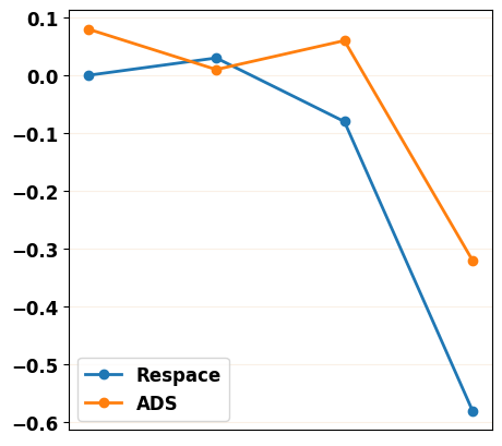
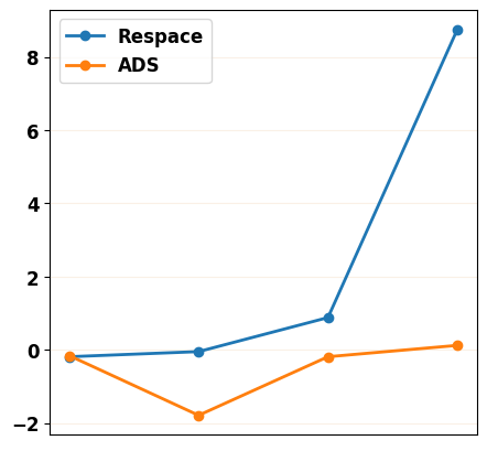
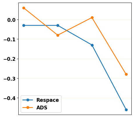
Table 14: Evaluation results of post-training based on models with different training steps, where “Begin” denotes the training steps and “Post” denotes the post-training steps.

F.5 Robustness of Adaptive Decay Sampling

To reflect the decrease of each evaluation metric along with fewer inference steps more clearly, we plot the rate of change for each metric in Figure 11. We can find that the change rate of our ADS strategy is lower than the Respace strategy, which means our method has better robustness as the number of down-sampled steps decreases.

Appendix G Human Evaluation

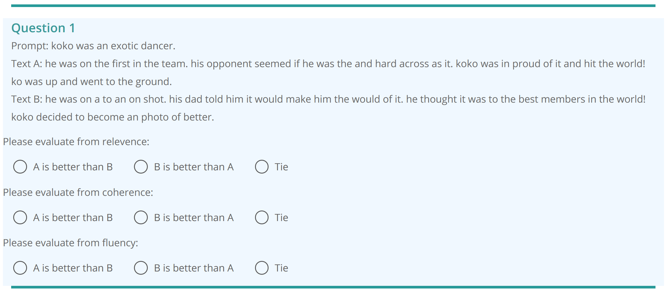
We show the statistic of human evaluation data in Table 11 and human evaluation interface in Figure 12 and 13. We build the human evaluation interface with the open-source python web library Django ¹⁸¹⁸18https://www.djangoproject.com. As shown in Figure 13, during the evaluation, each comparison pair contains one prompt and two corresponding outputs generated from two different models. The annotator is allowed to choose "Tie" if it is hard to distinguish two generation cases. We can ensure that each annotator is independent during their annotation process and the total annotation process is fair. We hired three annotators and payed each annotator $ 0.05 for comparing each pair. The payment is reasonable considering that it would cost average 30 seconds for an annotator to finish a comparison.

Appendix H Case Study

In this section, we present part of the generated results of each task for better illustration. We randomly select the cases generated by the diffusion model of 2,000 steps and 20 steps, and the diffusion model post-trained with the Distance Penalty method (2,000 steps) and ADS strategy (20 steps). For clear representation, we utilize green color denotes the key phrase related to the prompt, red color locates the phrase contradicts the prompt, and blue color highlights the serious grammatical errors. We can observe that, with our methods, the model can generate more fluency and high-quality texts, while the original model generates many repetitions or meaningless tokens. It is worth noting that the language model (pre-trained GPT-2) may allocate a good PPL score to the sentence with many repetition tokens, and those texts with massive meaning-less tokens or hard-to-read sentences may achieve a better Distinct and Lexical Repetition score.

Case	Type	Text
1	Prompt	i was on my laptop computer.
	Origin (2000)	all of a sudden my computer stopped working on the table. i was scared because it ripped so i ended up buying it. i went to the store to get a new one. after half of my computer, the screen were fine.
	+ Ours (2000)	all of a sudden my computer stopped working. the screen was broken. it was so frustrated i had to get a replacement. luckily i was able to fix.
	+ Respace (20)	all of a sudden my computer stopped and stopped working. i was very shocked and realized it was my computer. i called to the coffee again and had to buy a new one. after paying the work, my new computer broke.
	+ Ours (20)	all of a sudden my computer stopped. it broke the screen. it was not flying and i took it back to the store to fix it. luckily, it was fixed.
	Gold	i was writing a report for work. i was typing it up very quickly. my hands began to hurt. i took a break from the report.
2	Prompt	alex has a big exam on friday.
	Origin (2000)	he has been studying all week. he got out of class. he got into class instead. his teacher gave the test and knew and made an a.
	+ Ours (2000)	he has been studying all week. he got to class. when he got to class, his teacher handed out the test. alex was thrilled.
	+ Respace (20)	he has been studying all week. he got to class ready. he got into class. and his teacher got it. alex was chosen nervous and a slept.
	+ Ours (20)	he has been studying all week. he stayed up all night. he got to class days early. alex took the test and was so happy!
	Gold	he studied day in and day out. however, he didn’t take any breaks. this caused him to second guess his answers. he ended up failing the test because he over study.
3	Prompt	i went to the mall yesterday.
	Origin (2000)	i thought there was a sign sale. i ran off at the store. i found out it was one that sale. i was so upset.
	+ Ours (2000)	i thought there was a sale. so i walked up at the store. it was on sale. i was so upset.
	+ Respace (20)	i thought there was a sale. so i got up at the store. there was one sale. i was thrilled.
	+ Ours (20)	i thought there was a sale. so i went to the electronics store. there was a good sale. i was pleased with them.
	Gold	i tried on some lip gloss. it looked pretty. yet it burned my lips. i had to wipe it off.
4	Prompt	howard had his first baseball game.
	Origin (2000)	he was excited. when he went on the pitcher. he made sure he started to practice he would get. he did it in a display.
	+ Ours (2000)	he was very excited when he went on the game. he was nervous. at the moment he did he put it back. he ended up winning a day.
	+ Respace (20)	he was excited. when he went to the game. he got up at first. he got to beat - game. he did up a time.
	+ Ours (20)	he was very excited to try out in the game. he was nervous. when he started it, he found out he did. he did it in the park.
	Gold	he was very nervous. he ends up striking out. he left the game disheartened. his parents gave him cake to cheer him up.
5	Prompt	sara wanted to try out for the dance team.
	Origin (2000)	she was both nervous and excited. she often tried it but she didn’t know how try it. she finally decided to try out. she loved it, but and she both loved it.
	+ Ours (2000)	she was both nervous and excited. she had a years left and didn’t want to do it. she finally decided to try out. she made it and was glad she made it.
	+ Respace (20)	she was both nervous and excited. she had practiced late but she didn’t know how to others. she finally decided to try out. she tried it, but glad she was it
	+ Ours (20)	she was both nervous and excited. she had a routine, but didn’t know how to try. she finally decided to try out. she made it and was glad she made it.
	Gold	she started practicing every week. she was getting excited as tryouts got closer. on the day of tryouts, she was ready. when the list of who made it was posted, sara’s name was on it.
6	Prompt	susie wanted an ipad.
	Origin (2000)	she thought it would be great. finally she went her parents to get one. but when she opened it was gone. she couldn’t wait to use.
	+ Ours (2000)	she thought it would be fun. finally she convinced her parents to get one. when she opened it it was great. she couldn’t wait to buy it.
	+ Respace (20)	she thought it would be great. finally she convinced her family to get one. when she opened it up it was all great. she couldn’t even use it.
	+ Ours (20)	she thought it would be great. finally she convinced her parents to get one. when she opened it on it was beautiful. she couldn’t wait to use it.
	Gold	she begged for it. finally she looked under the tree. she saw one. she immediately hugged her parents.

Table 15: Representative generated results of the ROC testing set, where blue color denotes the serious grammatical errors.

Case	Type	Text
1	Prompt	the extinct volcano in the centre of edinburgh, capital city of scotland, has been known as arthur’s seat for centuries.
	Origin (2000)	what is the capital of : scotland
	+ Ours (2000)	what is the capital of : scotland
	+ Respace (20)	what is the capital of plane?
	+ Ours (20)	what is the capital of scotland?
	Gold	edinburgh castle stands on arthur’s seat what was arthur’s seat
2	Prompt	vergil in his wonderful poem, the aeneid, in two or three places, speaks of the queen of heaven, the goddess juno, as descending clothed with luminous light, and he uses the word nimbus for this
	Origin (2000)	ae was the luminous goddess of what
	+ Ours (2000)	what was the luminous goddess of greek with
	+ Respace (20)	who was the luminous goddess of what
	+ Ours (20)	how many was the greek goddess of light
	Gold	what’s the word for the luminous mist that surrounds a saint
3	Prompt	regulation time and overtime each game consists of three periods of twenty minutes each.
	Origin (2000)	there are minutes singer, how many in a game of?
	+ Ours (2000)	how many minutes is each period of hockey
	+ Respace (20)	what is the puck arery called in a game of hockey
	+ Ours (20)	how many minutes is each period of hockey
	Gold	how many minutes is each period of hockey?
4	Prompt	it is then dipped into powdered borax, and the adhering solid is held in the hottest part of the flame where it swells up as it loses its water of crystallization and then shrinks, forming a colourl
	Origin (2000)	what colour is hottests
	+ Ours (2000)	what colour is hottests
	+ Respace (20)	what colour is hottest featured into a govern
	+ Ours (20)	what colour is hottests
	Gold	when traces of a calcium compound are held in a bunsen flame, the colour of the flame changes to _ _ _?
5	Prompt	a name for the kestrel : cf. windhover.
	Origin (2000)	the windhover is the country name for which bird
	+ Ours (2000)	the windhover is an alternative name for which bird?
	+ Respace (20)	the windhover is the country name for which bird
	+ Ours (20)	the windhover is an alternative name for which bird?
	Gold	what is the moons astronomical name
6	Prompt	to help direct the path of light made available by clerestory windows, use light colored surfaces on your interior walls.
	Origin (2000)	what is the term for the path path of a body a weight
	+ Ours (2000)	what is the term for the path of a flag made in space
	+ Respace (20)	what is the term for the path followed by a body light?
	+ Ours (20)	path or trajectory of a annually, light by a credited.
	Gold	a row of windows in the upper part of a wall, especially in a church, to admit light below.

Table 16: Representative generation results on Quasar-T testing set, where blue color denotes the serious grammatical errors.

Case	Type	Text
1	Prompt	what are some of the pros and cons of a hillary clinton presidency?
	Origin (2000)	what are some of pros cons of hillary clinton presidency?
	+ Ours (2000)	what are the pros and cons of hillary clinton presidency?
	+ Respace (20)	what are pros and cons of \u201d and hillary clinton?
	+ Ours (20)	what are the pros and cons of hillary clinton?
	Gold	what are pros and cons of hillary clinton?
2	Prompt	which is less healthy for beer, your body?
	Origin (2000)	which is less healthy for your body, beer or pepsi?
	+ Ours (2000)	which one is better healthy, beer or pepsi?
	+ Respace (20)	which is less healthy healthy fors, beer or body?
	+ Ours (20)	which one is better for your body, beer or pepsi?
	Gold	which is less healthy for your body light beer or pepsi?
3	Prompt	is evolution real? how has this been proven?
	Origin (2000)	how evolution is real?
	+ Ours (2000)	how does evolution really exist?
	+ Respace (20)	is evolution really real?
	+ Ours (20)	is evolution really real?
	Gold	what are the different ways in which evolution has been proven to be real?
4	Prompt	how can i impress a girl who hate me?
	Origin (2000)	how can i impress a girl $[\cdots]$ ?
	+ Ours (2000)	what should i do to impress a girl hate me?
	+ Respace (20)	how do i impress a girl $[\cdots]$ ?
	+ Ours (20)	how do i impress a girl who hate me?
	Gold	how can impress a girl who hate me?
5	Prompt	what are the best and most effective openings in chess?
	Origin (2000)	what are the best effective \u201d in chess?
	+ Ours (2000)	what are the best effective openings in chess?
	+ Respace (20)	what are the best effective $[\cdots]$ in chess?
	+ Ours (20)	what are the best effective openings in chess?
	Gold	what are the best opening moves in chess?
6	Prompt	if you were given a chance to be somebody else for a day, who would you be?
	Origin (2000)	if you were a chance for his a day, who would you be?
	+ Ours (2000)	if you were given a chance to be somebody else for a day, who would you be?
	+ Respace (20)	if you were given in a day who will be else, who would it be?
	+ Ours (20)	if you were given a chance to be else for a day, who would you be?
	Gold	if you were given a chance to be somebody else for one day, who would you be?
7	Prompt	i want a real and effective way to make $ 500 per month with the knowledge that i have no money to invest?
	Origin (2000)	i want a real effective way to make 500 and $ knowledge per month?
	+ Ours (2000)	what is the best way to make $ 500 fast in india?
	+ Respace (20)	i want a real and 500 way to make \u201d her month?
	+ Ours (20)	i want a real way to make $ 500 month with the knowledge?
	Gold	the real effective way to make $ 500 per month with the knowledge that i have no money to invest?

Table 17: Representative generated results of the QQP testing set, where red color denotes the phrase contradicts the prompt, and blue color denotes the serious grammatical errors.

Case	Type	Text
1	Prompt	construction of changdeok palace began in 1405, and was completed in 1412.
	Origin (2000)	it was completed in 1412.
	+ Ours (2000)	construction of changdeok palace began in 1405, and was completed in 1412.
	+ Respace (20)	construction of changdeok palace began in 1405.
	+ Ours (20)	construction of changdeok palace began in 1405, and was completed in 1412.
	Gold (20)	The construction began by King Taejong, the Third King of the Joseon Dynasty, in 1405.
2	Prompt	however, this feature is not present in all cottontails nor is it unique to the genus.
	Origin (2000)	however, this feature is not present in all cottontails nor is it unique to the genus.
	+ Ours (2000)	however, this feature is not present in all cottontails nor is it unique to the genus.
	+ Respace (20)	however, this feature is not present in all cottontails nor is it unique to the genus.
	+ Ours (20)	however, this feature is not present in all cottontails nor is it unique to the genus.
	Gold (20)	However, this feature is not present in all cottontails.
3	Prompt	the team was owned by ralph wilson from the team’s founding in 1960, until his death in 2014 at the age of 95.
	Origin (2000)	the team was owned by ralph wilson from the team’s founding in 1960.
	+ Ours (2000)	the team was owned by ralph wilson from the team’s founding in 1960, until his death in 2014 at the age of 95.
	+ Respace (20)	the team was owned by ralph wilson from the team’s founding in 1960.
	+ Ours (20)	the team was owned by ralph wilson from the team’s founding in 1960.
	Gold (20)	Ralph Wilson, the longtime owner who had established the Bills in 1959, died on March 25, 2014.
4	Prompt	the association first convened in the 1960s, as interest increased in the new science of modern linguistics and particularly in its practical application - for example, in language teaching and learning.
4	Origin (2000)	the association first made in the 1960s.
	+ Ours (2000)	the association first convened in the 1960s, as interest increased in the new science of modern linguistics and particularly in its practical application - for example, in language teaching and learning.
	+ Respace (20)	the association first made in the 1960s as interest increased in the new science of modern linguistics.
	+ Ours (20)	the association first convened in the 1960s, as interest increased in the new science of modern linguistics and particularly in its practical application - for example, in language teaching and learning.
	Gold (20)	The association started in the 1960s.
5	Prompt	his hair shorn and now blind and shackled, samson is turning a mill - wheel and praying for his people, who will suffer for his sin.
	Origin (2000)	samson is turning a mill - wheel and who will suffer for his sin.
	+ Ours (2000)	his hair shorn and now blind and shackled, samson is turning a mill - wheel and praying for his people, who will suffer for his sin.
	+ Respace (20)	he is a mill - wheel for praying, who will suffer for his sin.
	+ Ours (20)	his hair shorn and now blind and shackled, samson is turning a mill - wheel and praying for his people, who will suffer for his sin.
	Gold (20)	He prays for his people.
6	Prompt	he was a significant figure in the development of ballroom dance during the first half of the 20th century, and his records sold 75 million copies from the 1930s through to the 1980s.
	Origin (2000)	his records sold 75 million copies from the 1930s through to the 1980s.
	+ Ours (2000)	he was a significant figure in the development of ballroom dance during the first half of the 20th century, and his records sold 75 million copies from the 1930s through to the 1980s.
	+ Respace (20)	he was a significant figure in the development of ballroom dance during the 20th century.
	+ Ours (20)	he was a significant figure in the development of ballroom dance during the first half of the 20th century.
	Gold (20)	He was a significant figure in the development of ballroom dance during the first half of the 20th century.
7	Prompt	alyosha monument, murmansk or defenders of the soviet arctic during the great patriotic war monument is also located in murmansk.
	Origin (2000)	alyosha monument, murmansk or defenders of the soviet arctic during the great patriotic war monument.
	+ Ours (2000)	alyosha monument, murmansk or defenders of the soviet arctic during the great patriotic war monument is also located in murmansk.
	+ Respace (20)	alyosha monument, murmansk or defenders of the soviet arctic during the great patriotic war monument.
	+ Ours (20)	alyosha monument, murmansk or defenders of the soviet arctic during the great patriotic war monument is also located $[\cdots]$ .
	Gold (20)	It is called the Alyosha Monument.
8	Prompt	singaporean citizens, government and non - governmental organisations may display or fly the national flag throughout the year to identify themselves with the nation, and especially encouraged to do so during occasions of national celebration or national significance.
	Origin (2000)	singaporean citizens, government and non - governmental organisations may display or fly the national flag throughout the year to identify themselves with the nation.
	+ Ours (2000)	singaporean citizens, government and non - governmental organisations may display or fly the national flag throughout the year to identify themselves with the nation, and especially encouraged to do so during occasions of national celebration or national significance.
	+ Respace (20)	singaporean citizens, government and non - governmental organisations may display or fly the national flag throughout the year to identify themselves with the nation.
	+ Ours (20)	singaporean citizens, government and non - governmental organisations may display or fly the national flag throughout the year to identify themselves with the nation.
	Gold (20)	Singaporeans are encouraged to do this during occasions of national celebration or national significance.

Table 18: Representative generated results of the WIKI-AUTO testing set, where red color denotes the phrase contradicts the prompt, and blue color denotes the serious grammatical errors. We can observe that our method can generate much shorter and streamlined content.

Case	Type	Text
1	Prompt	name : The Vaults
	Origin (200)	The Vaults Two is a family friendly Italian restaurant .
	+ Ours (200)	The Vaults is a cheap , family friendly Italian restaurant .
	+ Respace (20)	The Plough is a cheap , family friendly pub near Caf\u00e9 Rouge .
	+ Ours (20)	The Vaults is a family friendly fast food restaurant .
2	Prompt	name : The Cambridge Blue
	Origin (200)	The Cambridge Blue provides Indian food Its customer rating is low .
	+ Ours (200)	The Cambridge Blue is a restaurant that serves Italian food .
	+ Respace (20)	Browns Cambridge is a 5 star dine in restaurant . It is moderately priced .
	+ Ours (20)	The Cambridge Blue is a restaurant with a high customer rating .
3	Prompt	name : The Golden Palace
	Origin (200)	The Mill is a coffee shop that serves Italian food, is located in riverside near The Sorrento .
	+ Ours (200)	The Golden Palace is a high priced coffee shop serving Indian food located in the city centre with a customer rating of 1 out of 5 .
	+ Respace (20)	The Golden Palace is a Japanese coffee shop with a moderate price range in the city centre . 1 out of 5 customer rating .
	+ Ours (20)	The Golden Palace is a fast food coffee shop in the city centre that has a moderate price range and a customer rating of 1 out of 5 .
4	Prompt	Type : pub
	Origin (200)	Blue Spice provides Chinese food in the high price range . It is located in the city centre .
	+ Ours (200)	The Olive Grove is a pub providing Chinese food It is located in the city centre .
	+ Respace (20)	Wildwood , a pub serving French food with a customer rating of low .
	+ Ours (20)	The Mill is a pub that provides Indian food It is in the cheap price range . It is located in riverside .
5	Prompt	near : Clare Hall
	Origin (200)	There is a cheap family friendly Japanese restaurant called Loch Fyne . \n END near Clare
	+ Ours (200)	Bibimbap House is a Chinese restaurant in the high price range . It is located in the riverside area near Clare Hall .
	+ Respace (20)	This restaurant Bibimbap House Clare Hall is a cheap and located in the city that serves Japanese food .
	+ Ours (20)	Clowns is a coffee shop by the riverside near Clare Hall and has a customer rating of 3 out of 5 .
6	Prompt	near : The Six Bells
	Origin (200)	Near The Six Bells is Fitzbillies , , cheap , which serves English food .
	+ Ours (200)	Fitzbillies is a moderately priced Italian restaurant located near The Six Bells .
	+ Respace (20)	Near The Six Bells , Giraffe a moderately priced restaurant .
	+ Ours (20)	Giraffe is a restaurant near The Six Bells with a high price range .
7	Prompt	family friendly : yes
	Origin (200)	The Eagle is a fast food restaurant that is highly rated
	+ Ours (200)	Loch Fyne is a family friendly restaurant that serves English food .
	+ Respace (20)	Zizzi is a , 1 star restaurant , it offers spirits , and it is family friendly
	+ Ours (20)	The Cricketers is a family friendly coffee shop serving Japanese food . It is located near The Portland Arms with a customer rating of 5 out of 5 .
8	Prompt	food : Chinese
	Origin (200)	The Wrestlers provides Chinese food in the moderate price range .customer rating is 1 out of 5 .
	+ Ours (200)	The Waterman is providing Chinese food in the cheap price range . It is located in the riverside . Its customer rating is 5 out of 5 .
	+ Respace (20)	Browns Cambridge sells Japanese food , for 20 - 25 , with a customer rating 3 out of 5
	+ Ours (20)	The Waterman provides Chinese food in the cheap price range . It is located in the riverside . Its customer rating is average .

Table 19: Representative generated results of the E2E (Semantic Content) testing set, where green color denotes the key phrase related to the prompt, red color denotes the phrase contradicts the prompt, and blue color denotes the serious grammatical errors.

Case	Type	Text
1	Prompt	[3, 5, PP]
	Origin (200)	Browns Cambridge is in the city centre near The Sorrento . It is a family - friendly restaurant .
	+ Ours (200)	In city centre near Clare Hall , there is a coffee shop called Clowns . It also serves Italian food and has a customer rating of 5 out of 5 .
	+ Respace (20)	Browns Cambridge is on the riverside near The Sorrento . It is a family friendly restaurant serving English food .
	+ Ours (20)	Aromi is located in the city centre and is a family - friendly coffee shop that serves Italian food with a low customer rating .
	Gold	Only feet away from Caf0̆0e9 Sicilia , The Punter coffee Shop offers low price coffee and does not have family restrooms .
2	Prompt	[5, 7, NP]
	Origin (200)	Cotto provides Indian food It is near Ranch . Its customer rating is average .
	+ Ours (200)	In the city centre near The Portland Arms , there is a coffee shop called Cotto . It serves Italian food . It has a high price range and a customer rating of 1 out of 5 .
	+ Respace (20)	The Vaults is a restaurant providing Italian food in the high price range .
	+ Ours (20)	In the city centre near Crowne Plaza Hotel is a fast food coffee shop named Browns Cambridge . It has a customer rating of 5 out of 5 and is family - friendly .
	Gold	For date night go to The Rice Boat , cheap , average rated Chinese not family friendly food near Express by Holiday Inn
3	Prompt	[6, 9, ADVP]
	Origin (200)	Blue Spice provides Chinese food in the high price range . It is located in the city centre .
	+ Ours (200)	Cotto is a cheap restaurant located near All Bar One
	+ Respace (20)	The Plough is a cheap Italian pub near Caf\u00e9 Rouge . It is family friendly .
	+ Ours (20)	Clowns is a coffee shop located next to Clare Hall .
	Gold	Browns Cambridge located in city centre close to The Sorrento serves Indian food . It is a adult dining restaurant .
4	Prompt	[10, 11, PP]
	Origin (200)	Aromi is a coffee shop that is rated 5 out of 5 and serves French food . It is not family - friendly . It is located in the city centre .
	+ Ours (200)	The Rice Boat is located near Express by Holiday Inn in riverside . It is a family - friendly Japanese restaurant with a low customer rating and a low price range .
	+ Respace (20)	The Twenty Two offers Japanese food in a family - friendly environment . It is located in the city centre .
	+ Ours (20)	The Eagle coffee shop has a rating of 5 out of 5 . It is a family friendly Fast food place in the city centre , near Burger King .
	Gold	Highly rated English food restaurant The Waterman , is located in Riverside . The cost is high but is not child friendly .
5	Prompt	[0, 0, NP]
	Origin (200)	There is a family friendly Japanese restaurant in the riverside area near The Sorrento , named Browns Cambridge .
	+ Ours (200)	Fitzbillies is a coffee shop providing Indian food in the high price range . It is located in the city centre . Its customer rating is 1 out of 5 .
	+ Respace (20)	There is a kid - friendly fast food restaurant in Riverside called The Twenty Two .
	+ Ours (20)	Wildwood is a coffee shop providing Indian food in the moderate price range . It is near Ranch . Its customer rating is 1 out of 5 .
	Gold	There is a family friendly coffee shop located close to the Crowne Plaza Hotel . It is called Browns Cambridge .
6	Prompt	[4, 6, NP]
	Origin (200)	Taste of Cambridge is a coffee shop that serves Japanese food . It is located in the riverside area near Crowne Plaza Hotel . It is not family - friendly .
	+ Ours (200)	The Eagle is a a coffee shop that provides Indian food in the high price range . It is located in the riverside . It is near Burger King . Its customer rating is 1 out of 5 .
	+ Respace (20)	Alimentum is located in the city centre and serves Japanese food . It is kid friendly and has a price range of 0̆0a3 20 - 25 .
	+ Ours (20)	The Rice Boat is a Japanese restaurant located in the city centre near the Express by Holiday Inn . It is kid friendly and has a price range of 20 - 25 . It has a customer rating of 3 out of 5 .
	Gold	The Golden Palace is a coffee shop with Italian food , prices less then 20 , in the riverside and has low ratings .

Table 20: Representative generated results of the E2E (Syntax Spans) testing set, where green color denotes the key phrase related to the prompt, red color denotes the phrase contradicts the prompt, and blue color denotes the serious grammatical errors.