Can distributed delays perfectly stabilize dynamical networks?

Oscillation is not omnipresent in the brain, but is observed only in limited areas such as the cat visual cortex and the olfactory bulb oscillation . Extensive synchronization occurs in rather pathological conditions such as parkinsonian tremor or epilepsy synchronization . How is the collective oscillation avoided in the brain composed of neurons that are prone to synchronize?

Recently it has been revealed that distributed delays in the signal transmission contribute toward stabilization, in neural networks gong07 ; omi07 , ecological systems eurich03 ; eurich05 , control engineering control , biology macdonald89 or coupled dynamical systems cds . In the light of this knowledge, wide distributions of neuronal signal transmission delays reported recently delay bear apparent consistency with the absence of extensive oscillation in the brain.

Conversely, the signal transmission delay itself is known to be a destabilizing factor instable . We therefore wish to comprehend how these factors are competing in real dynamical systems; in particular, how the macroscopic stability of dynamical systems is controlled by the dispersion of delays and their average.

For this purpose, we examine the stability of an integro-differential equation macdonald89 ; delay-equation derived from microscopic dynamics of a neural network whose signal transmission delays are distributed in time. It is revealed from the analysis that the network with gamma distributed delays less dispersed than exponential distribution exhibits reentrant stability; the system once destabilizes but then recovers the stability as the average delay is increased. With delays dispersed more highly than exponential distribution, the system attains a perfect macroscopic stationarity.

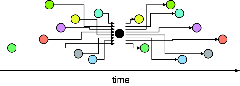
We consider a network of model neurons that obey the evolution equation,

where $\textrm{sgn}(v)$ is the sign function that takes values $+1$ and $-1$ respectively for $v>0$ and $v\leq 0$. $\tau$ is the “membrane time constant” of an individual neuron. The “synaptic weight” $w_{i,j}$ and the signal transmission delay $d_{i,j}$ are fixed to each transmission line from $j$th neuron to $i$th neuron (Fig.1). $s_{i}$ is the “external stimulus” to each neuron.

A dynamical equation of the macroscopic order parameter $X(t)\equiv\frac{1}{n}\sum_{i=1}^{n}x_{i}(t)$ can be derived in a manner similar to what we have done for the discrete time model omi07 in parallel with Amari’s derivation for the synchronous update rule amari71 : A mean field exerted on $X(t)$ is given by the difference of ratios of positive and negative inputs. Using the distribution $p_{t}(v)$ of inputs $\{v_{i}=\sum_{j=1}^{n}w_{i,j}x_{j}(t-d_{i,j})+s_{i}\}$ at time $t$, the macroscopic equation can be represented as

Under the assumption of the statistical independence of $\{x_{j}(t-d_{i,j})\}$ from $\{w_{i,j}\}$, the central limit theorem holds for the summed inputs $\{\sum_{j=1}^{n}w_{i,j}x_{j}(t-d_{i,j})\}$. If in addition $\{s_{i}\}$ are normally distributed, the distribution $p_{t}(v)$ can be approximated as Gaussian characterized solely by the mean and the variance at time $t$. Then, the macroscopic state equation is obtained as

where $F(x)$ is the error function

and $I$ is the ratio of the mean and the standard deviation of inputs $\{v_{i}\}$ to neurons

where $\mu_{w}$, $\mu_{s}$, $\sigma^{2}_{w}$ and $\sigma^{2}_{s}$ are respectively the means and variances of $\{w_{i,j}\}$ and $\{s_{j}\}$.

Under the assumption that microscopic states $\{x_{i}\}$ are statistically independent from delays $\{d_{i,j}\}$, the mean past activity $\langle x\rangle\equiv\frac{1}{n^{2}}\sum_{i=1}^{n}\sum_{j=1}^{n}x_{j}(t-d_{i,j})$ can be represented by the macroscopic order parameter omi07 as

where $g(s)$ represents the distribution of delays. $\langle x^{2}\rangle\equiv\frac{1}{n^{2}}\sum_{i=1}^{n}\sum_{j=1}^{n}x^{2}_{j}(t-d_{i,j})$ remains close to unity, if individual microscopic states are always approaching swiftly either of $\pm 1$.

If $n(\sigma^{2}_{w}+\mu^{2}_{w})\ll\sigma^{2}_{s}$, or if $\langle x^{2}\rangle$ can be approximated as unity, then the dynamical equation (3) is closed with the macroscopic order parameter $X(t)$. Furthermore, if the model parameters satisfy $n\mu_{w}^{2}\ll n\sigma_{w}^{2}+\sigma_{s}^{2}$, the evolution equation simplifies to

where $W=n\mu_{w}/\sqrt{n\sigma_{w}^{2}+\sigma_{s}^{2}}$ and $S=\mu_{s}/\sqrt{n\sigma_{w}^{2}+\sigma_{s}^{2}}$. Note that $n\mu_{w}^{2}\ll n\sigma_{w}^{2}+\sigma_{s}^{2}$ is not an essential condition for a macroscopic equation (7) to hold but is merely introduced to make the analysis simpler.

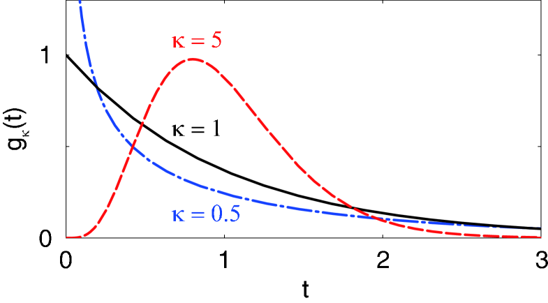
With this integro-differential equation, we investigate the influence of the dispersed delays on the macroscopic stability of the system. We adopt here the gamma distributed delays,

which is characterized by the scale factor $T$ representing the average delay, and the shape factor $\kappa$ representing (inversely related to) the dispersion of delays. $\Gamma(\kappa)$ is the gamma function defined by $\int_{0}^{\infty}x^{\kappa-1}e^{-x}dx$.

Given a macroscopic stationary state $X(t)=X_{0}$ that satisfies $X_{0}=F\left(WX_{0}+S\right)$, we examine the linear stability with respect to the deviation from the stationary state, by putting $X(t)-X_{0}=\exp(\lambda t/\tau)$. The characteristic equation for the linearized integro-differential equation is obtained as

where $\beta$ represents the slope of the response function,

For positive $\beta$, the system exhibits instability, $\lambda\geq 0$, if the response function $F(WX+S)$ has a slope greater than unity, $\beta>1$. In this case, the system eventually attains one of stable stationary states due to the nonlinear saturation.

A dynamical instability leading to oscillation may take place for negative $\beta$. In this case, the linear-stability boundary is obtained by solving a pair of simultaneous equations that represent the condition for the characteristic equation (9) to have a pure imaginary solution $\lambda=i\omega$:

Equation (11) has a solution only if $\kappa>1$. In the limit of $T/\tau\to 0$, $\omega$ is obtained as

and critical $\beta$ is obtained from Eq.(12) as

In the opposite extreme of $T/\tau\to\infty$, $\omega$ is obtained as

with which the critical $\beta$ is obtained respectively as

Figure 3 depicts the stability boundaries in the phase space of $\{T/\tau,-\beta\}$ obtained by numerically solving Eqs.(11) and (12) for several shape parameters $\kappa$: With identical delays ($\kappa\to\infty$), the critical coupling strength $|\beta|$ decreases monotonically with the average delay $T$. In other words, the system becomes more fragile with delays. This fact is consistent with the knowledge that the transmission delay is a destabilizing factor. It is notable that a system with dispersed delays exhibits reentrant phenomena; the stability is once lost but then recovered as the average delay $T$ is increased: With the delays of small dispersion ($2<\kappa<\infty$), the critical $|\beta|$ rebounds and then saturates to a finite value. In a middle range of dispersion ($1<\kappa\leq 2$), the critical $|\beta|$ takes a minimum and diverges with $T$. With the delays highly dispersed ($\kappa\leq 1$), the network never destabilizes.

Next, we numerically solve the macroscopic evolution equation (7) to see if there is nontrivially coexisting oscillation or chaos in the parameter range in which the linear stability is confirmed. For this purpose, we have tested a number of random initial conditions of various power spectra; from white (jagged) to colored (smooth) random temporal patterns.

Solving an integro-differential equation is generally a hard computational task. In some particular conditions, however, the computational complexity can be reduced drastically by devising efficient algorithms: For the exponential distribution of delays ($\kappa=1$), the mean past activity $\int_{0}^{\infty}e^{-s}X(t-s)ds$ is represented by

where $\Delta$ is a unit step. Due to the exponential kernel, $A_{t}$ can be obtained by simply iterating the recurrence equation:

In addition, for the case of $\kappa=2$, the computational complexity could be reduced by utilizing the relation of

with sufficiently small $|\varepsilon|$.

To the extent we have exhausted, we have not found any non-trivial coexisting dynamical orbits in the parameter range that the linear stability is guaranteed. Figure 4 shows an amplitude of $X(t)$ obtained for the systems with shape parameters of $\kappa=2$ and $1$. In the case of $\kappa=2$, a significant amplitude of $X(t)$ can be observed in the interval of mean delay $T$ in which the system is linearly unstable. For the shape parameter $\kappa=1$ with which the system is linearly stable, the amplitude is negligibly small in the whole range of $T$.

What is the key factor in the perfect stability? As the system shows a perfect stability in the absence of delay, we suspect if a fraction of instantaneous signal transmissions lead to the stability for $\kappa\leq 1$. We examine the stability of a system with the delay distribution composed of two delta functions peaked at zero and finite delays, $a\delta(t)+(1-a)\delta(t-T)$. It is found from the characteristic equation that the system can be destabilized even if delay-less lines are present in a finite fraction, $0\leq a<1/2$. This fact demonstrates that the presence of instantaneous signal transmissions alone does not necessarily induce a perfect stability.

Next, we suspect if the long tail of the delay distribution has led to the stability. We examine whether or not a system remains stable even if a lag is added to gamma distributed delays (8) as $\theta(t-\epsilon)g(t-\epsilon)$, where $\theta(x)$ is the Heaviside step function: $\theta(x)=1$ if $x\geq 0$ and $=0$ otherwise. In the presence of a lag, $\epsilon>0$, the instability condition Eq.(11) is modified as

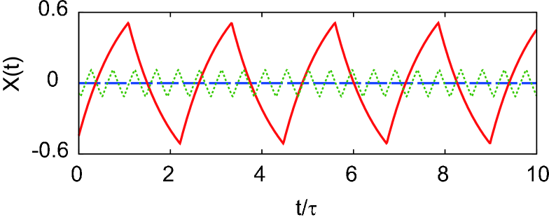
This characteristic equation possesses a solution even for the case of a high dispersion, $\kappa\leq 1$. This implies that the perfect stability can be destroyed by a time lag. As long as the time lag $\epsilon$ is small, however, the system exhibits an instability at a very high frequency of the order of $\tau\pi/\epsilon$, and the amplitude of the order parameter $X(t)$ cannot grow large due to the nonlinearity of the system. This point is verified by directly solving the original nonlinear macroscopic evolution equation. Figure 5 compares the order parameters $X(t)$ computed for the several kinds of delay distributions: the system of $\kappa=2$ may exhibit a large amplitude $X(t)$; the system of $\kappa=1$ has never yielded a significant amplitude $X(t)$; the system with gamma distributed delays of $\kappa=1$ accompanied by a small time lag $\epsilon/\tau=0.01$ has yielded an order parameter $X(t)$ rapidly oscillating with a small amplitude.

In the present study, we examined the stability of a neural network whose signal transmission delays are distributed in time. The network is found to exhibit a reentrant stability for the delays less dispersed than the exponential distribution. The network attains a perfect stability for the highly dispersed delays. It is noteworthy that Eurich et al also proved that the perfect stability is attained in the limit of highest dispersion, $\kappa=0$, for an ecological feedback system eurich05 . In this Letter, we have revealed that the perfect stability is manifested in a finite range of the dispersion or the shape parameter, $0<\kappa\leq 1$, for a neural network. It is desirable to examine the generality of the present findings; whether or not the perfect stability is achieved solely due to the delay distribution, irrespective of detailed dynamics of individual elements.

References

- (1) C. M. Gray, P. König, A. K. Engel and W. Singer, Nature (London) 338, 334 (1989); G. Laurent and H. Davidowitz, Science 265, 1872 (1994).
- (2) P. J. Uhlhaas and W. Singer, Neuron 52, 155 (2006)
- (3) P. Gong and C. van Leeuwen, Phys. Rev. Lett. 98, 048104 (2007).
- (4) T. Omi and S. Shinomoto, Phys. Rev. E 76, in press (2007).
- (5) A. Thiel, H. Schwegler and C. W. Eurich, Complexity 8, 102 (2003).
- (6) C. W. Eurich, A. Thiel and L. Fahse, Phys. Rev. Lett. 94 (2005) 158104.
- (7) J. E. S. Socolar and D. J. Gauthier, Phys. Rev. E 57, 6589 (1998); A. Ahlborn and U. Parlitz, Phys. Rev. Lett. 93, 264101 (2004).
- (8) N. MacDonald Biological delay systems: linear stability theory, (Cambridge University Press, New York, 1989).
- (9) F. M. Atay, Phys. Rev. Lett. 91, 094101 (2003); V. K. Jirsa and M. Ding, Phys. Rev. Lett. 93, 070602 (2004); C. Masoller and A. C. Marti, Phys. Rev. Lett. 94, 134102 (2005); A. C. Marti, M. Ponce and C. Masoller, Phys. Rev. E 72, 066217 (2005); D. Huber and L. S. Tsimring, Phys. Rev. E 71, 036150 (2005).
- (10) H. A. Swadlow, J. Neurophysiol. 54, 1346 (1985); J. G. Pelletier and D. Paré, J. Neurophysiol. 87, 1213 (2002); A. F. Soleng, M. Raastad and P. Andersen, Hippocampus 13, 953 (2003).
- (11) M. C. Mackey and L. Glass, Science 197, 287 (1977); K. Ikeda and K. Matsumoto, Physica D 29, 223 (1987); C. M. Marcus and R. M. Westervelt, Phys. Rev. A 39, 347 (1989).
- (12) M. N. Oǧuztöreli Time-Lag Control Systems, (Academic Press, New York, 1966); J. K. Hale and S. M. V. Lunel, Introduction to Functional Differential Equations, (Springer-Verlag, New York, 1993).
- (13) S. Amari, Proc. IEEE 59, 35 (1971); W. Kinzel, Z. Phys. B 60, 205 (1985); S. Shinomoto, Prog. Theor. Phys. 75, 1313 (1986); S. Shinomoto, Biol. Cybern. 57, 197 (1987).