Canonical sectors and evolution of firms in
the US stock markets
Abstract
A classification of companies into sectors of the economy is important for macroeconomic analysis and for investments in sector-specific financial indices and exchange traded funds (ETFs). Major industrial classification systems and financial indices have historically been based on expert opinion and developed manually. Here we show how unsupervised machine learning can provide a more objective and comprehensive broad-level sector decomposition of stocks. An emergent low-dimensional structure in the space of historical stock price returns automatically identifies ’canonical sectors’ in the market, and assigns every stock a participation weight into these sectors. Furthermore, by analyzing data from different periods, we show how these weights for listed firms have evolved over time.
keywords:
Machine Learning, Archetypal Analysis, Canonical Sectors, Computational FinanceContact Information
-
•
Lorien X. Hayden
-
–
(573) 819-2155
-
–
lxh3@cornell.edu
-
–
-
•
Ricky Chachra
-
–
(212) 729-7529
-
–
rickychachra@gmail.com
-
–
-
•
Alexander A. Alemi
-
–
(814) 422-5364
-
–
alexalemi@gmail.com
-
–
-
•
Paul H. Ginsparg
-
–
(607) 255-7371
-
–
ginsparg@cornell.edu
-
–
-
•
James P. Sethna
-
–
(607) 275-7748
-
–
sethna@lassp.cornell.edu
-
–
Acknowledgements
We thank Jean–Philippe Bouchaud, Ming Huang and Janet Gao for helpful discussions.
Funding
This work was partially supported by NSF grants DMR-1312160, DMR-1719490, IIS-1247696 and DGE-1144153.
Abstract
C38, G10
Main Text
Stock market performance is measured with aggregated quantities called indices that represent a weighted average price of a basket of stocks. Market-wide indices such as Russell 3000® (Russell 3000® Index, 2015) and the S&P 500® (S&P 500® Index, 2014) consist of stocks from diverse companies reflecting a broad cross-section of the market. Sector-specific indices such as the Dow Jones® Financials Index (Dow Jones® US Indices: Industry Indices, 2015), CBOE® Oil Index (CBOE® Oil Index, 2013) and the Morgan Stanley® High-Tech 35 Index (Morgan Stanley® High-Tech 35 Index, 2005), etc., are more granular and their composition requires a classification of companies into sectors. Major industrial classification schemes classify firms into sectors, albeit with many ambiguities (Nadig and Crigger, 2011). It is not clear, for example, how to assign a sector to conglomerates or diversified companies such as General Electric®. Conversely, non-conglomerates with exposure to firms outside their own sector (for example, an investment bank exclusively serving pharmaceutical firms) also blur the boundaries of sector-identification. Moreover, as companies and their economic environments evolve, neither the industrial sectors nor the firms’ sector association remains static, necessitating updates to sector assignments and addition of new sectors.
A significant number of studies have previously aimed at identifying categories of stocks in financial markets with a variety of approaches. Recent numerical techniques have included extensive use of random matrix theory, principal component analysis or associated eigenvalue decomposition of the correlation matrix (Plerou et al., 2002; Kim and Jeong, 2005; Fenn et al., 2011; Conlon et al., 2009; Eom et al., 2007; Coronnello et al., 2005), specialized clustering methods (Mantegna, 1999; Bonanno et al., 2000, 2003; Heimo et al., 2009; Basalto et al., 2005; Kullmann et al., 2000; Musmeci et al., 2014) or time series analysis (Podobnik and Stanley, 2008; Martins, 2007), pairwise coupling analysis (Bury, 2013), and even topic-modeling of returns (Doyle and Elkan, 2009). Indeed, relevant prior work analyzing historical stock price returns (Laloux et al., 1999; Plerou et al., 2002; Fama and French, 1993) elucidated that the high-dimensional space of stock price returns has a low-dimensional representation.
In parallel with this, there is a long tradition of style analysis in finance in which time series can be selected which serve as useful benchmarks for the performance of other stocks or indices. The three-factor model of Fama and French (Fama and French, 1993) is one such example. Recently, D. Vistocco and C. Conversano (Vistocco and Conversano, 2009) proposed that Archetypal Analysis (AA) (Cutler and Breiman, 1994) could provide these benchmark time series while also providing a way to plot this data in a meaningful way. In particular, they provide a triangular plot for Italian mutual funds and suggest parallel coordinate plots or asymmetric maps for higher dimensional representations. The positive decomposition of mutual funds into sectors using standard benchmarks (not derived using AA) was later studied by the same authors (Conversano and Vistocco, 2010).
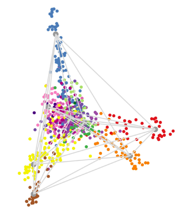
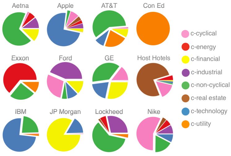
Here, we demonstrate a new, holistic way of classifying stocks into industrial sectors by utilizing the emergent structure of price returns in data space. Beyond the proposal of Vistocco and Conversano, we provide an interpretation of the archetypes of AA as sectors of the economy. This structure is purely contained in the geometry of the time series. Other methods, such as SVD, can discern that there is some such structure but are not well suited to a clean description. Archetypal Analysis, on the other hand, determines the convex hull of the dataset making it uniquely suited to creating a quantitative analysis of the data. In particular, if we take the log price returns of individual stocks, remove the overall market return, normalize to zero mean and unit s.d., then stock returns are well-approximated by a hyper-tetrahedral structure. Each lobe of the hyper-tetrahedron is populated by stocks of similar or related businesses (Fig. 1); the lobe-corners (canonical sectors) approximate the returns of companies that are prototypical of individual sectors (Table Main Text). Returns of each stock can be decomposed into a weighted sum (Fig. 2) of the canonical sector returns (Fig. 3). Lastly, the canonical sector weights for a given company are dynamic and lead to insights into its evolution (Fig. 5).
Canonical sectors and major business lines of primary constituent firms. The eight canonical sectors identified by the analysis described here are listed in the column on the left; these were named in accord with the business lines (middle column) of firms that show strong association with these sectors. Some examples are provided in the right column; a full list is available on companion website (Chachra et al., 2013). Canonical sector Business lines Prototypical examples c-cyclical general and specialty retail, discretionary goods Gap, Macy’s, Target c-energy oil and gas services, equipment, operations Halliburton, Schlumberger c-financial banks, insurance (except health) US Bancorp., Bank of America c-industrial capital goods, basic materials, transport Kennametal, Regal–Beloit c-non-cyclical consumer staples, healthcare Pepsi, Procter & Gamble c-real estate realty investments and operations Post Properties, Duke Realty c-technology semiconductors, computers, comm. devices Cisco, Texas Instruments c-utility electric and gas suppliers Duke Energy, Wisconsin Energy
The matrix of daily log returns of a stock are defined as where are adjusted closing prices (i.e. corrected for stock splits and dividend issues) and is in trading days. In the present analysis, we used normalized returns, , where is the variance (squared volatility) and represents the average over time (trading days). Overall market returns from each stock were also removed, yielding what we shall call the log price returns . (The two degrees of freedom we remove from each stock – the variance and the overall return – are of practical interest elsewhere, but obscure the classification into sectors.) The hyper-tetrahedron, or simplex, which emerges (Fig. 1) is a self-organized structure: it has prototypical firms in corners (Table Main Text), closely related firms clumped together in each lobe, diversified companies (GE®, Walt Disney®, 3M®, etc.) close to the center, and the number of lobes denoting how many distinct sectors are exhibited by the data. This suggests a natural way to decompose stocks into canonical sectors: for convex sets, each interior point is representable as a unique weighted sum of corner points, implying here that every stock’s return is approximated by a weighted sum of returns from the canonical sectors. Conversely, the weights for a given stock quantify its exposure to the canonical sectors.
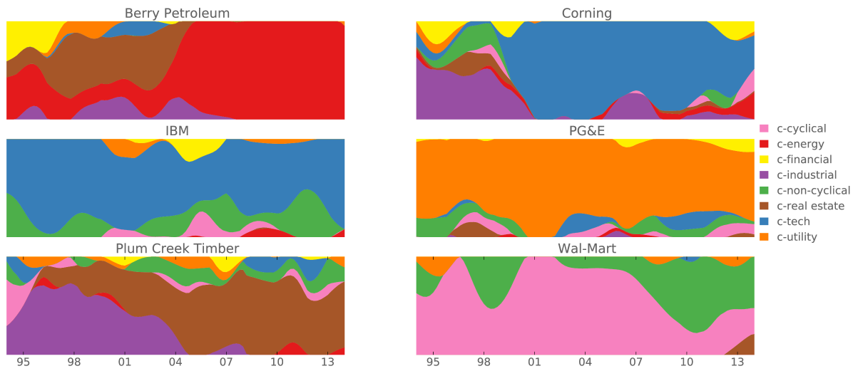
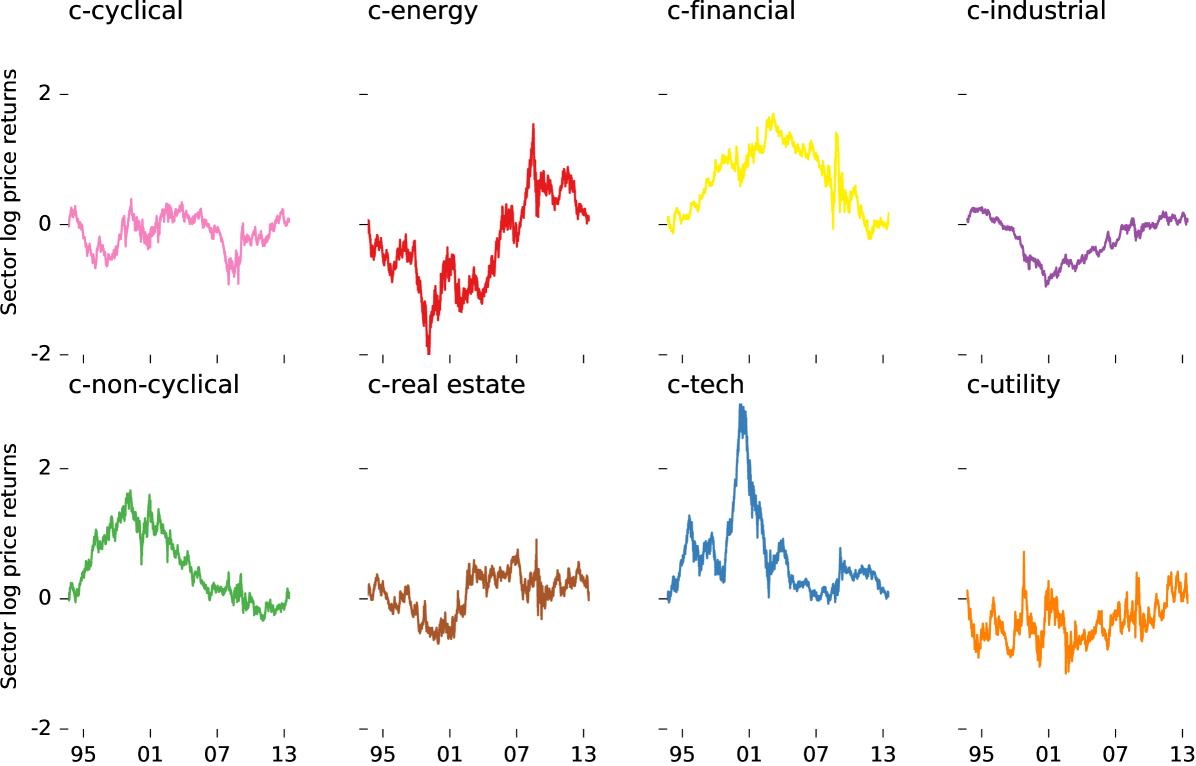
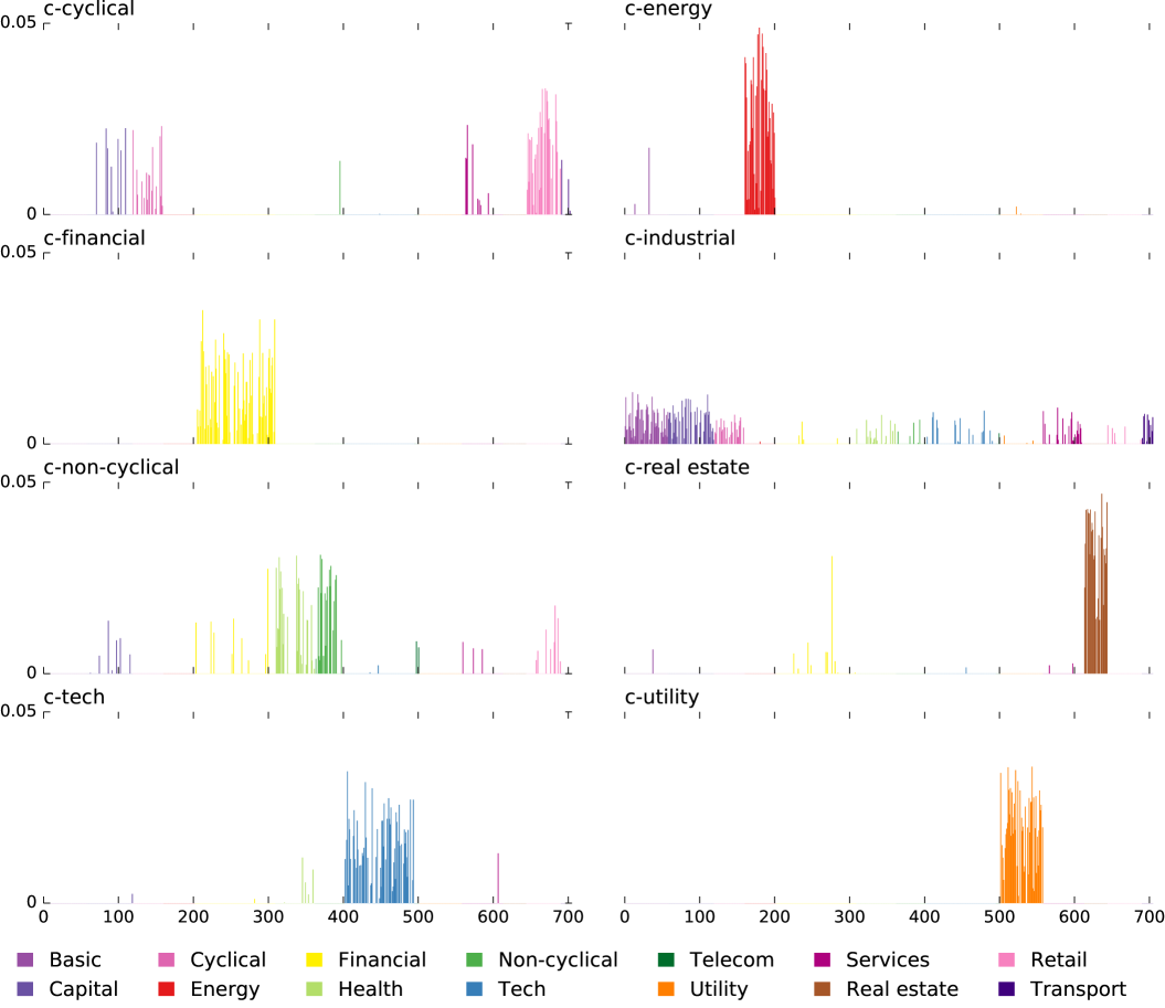
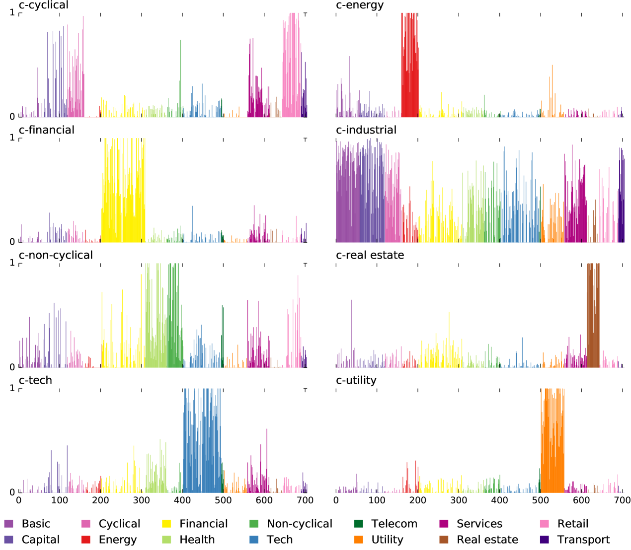
We applied an in house python implementation of the AA algorithm described by Mørup and Hansen (Mörup and Hansen, 2012). The dataset consisted of 705 US firms’ stocks with a minimum $1 billion June 2013 market capitalization and with continuous 20 years (1993–2013) of listing on major exchanges (Appendix A). Analysis of this dataset (Appendices B and C) revealed eight emergent sectors which were named in accordance with the companies they comprised (prefix c- denotes “canonical”): c-cyclical (including retail), c-energy (including oil and gas), c-industrial (including capital goods and basic materials), c-financial, c-non-cyclical (including healthcare and consumer non-cyclical goods), c-real estate, c-technology, and c-utility. Calculated participation weights for a sample of 12 firms in Fig. 2 show a decomposition of their stocks into the canonical sectors with resulting insights discussed in the caption. Associated with each canonical sector is a time series of returns. As expected, these series show hallmark historical events of individual sectors (Fig. 3): the dot-com bubble, the energy crisis, and the financial crisis being the major events in the last two decades.
Determining the correct number of canonical sectors that appropriately describe the space of stock market returns is akin to the more general issue of selecting a signal-to-noise ratio cutoff, or a truncation threshold in the dimensional-reduction of data. The choice of this threshold is generally sensitive to sampling, yet the results presented here are reasonably robust with different choices leading to meaningful and similar decompositions. Fig. 4 depicts the changes in the decomposition with dimension. Details of how the figure was generated as well as more information on the two and three dimensional decompositions are available in Appendix G.
In addition to the full data set of 20 years 705 firms, we also applied the algorithm to overlapping, two-year Gaussian windows to study how the sector weights for firms have evolved in time (Fig. 5, see also Appendix C). As expected, the sector decomposition of firms is dynamic. Mergers, acquisitions, spin-offs, new products, effect of competitive environments or shifting consumer preferences can change the business foci of firms and hence alter the sector association of firms. External events affecting companies in an idiosyncratic manner also show clear signature in this analysis.
The eight-factor decomposition presented here explains 11.1% of the total variation () in the normalized returns with the market mode removed, and 56% of the random matrix theory explainable variation defined in Appendix F. For comparison, the classic three-factor decomposition of portfolio returns by Fama and French (Fama and French, 1993) into market mode, market capitalization, and growth versus value yields an value of only 4.75%. Indeed, if only three factors are used instead of the eight for the decomposition presented here, the regression yields a comparable value (5.61%) but there appears to be no correspondence between three factors found by our unsupervised model, and those of Fama and French (Fig. 14). Carrying out a similar comparison with Fama and French’s analysis applied to model portfolio returns, the regression on the S&P 500® yields an value of 99.4% for Fama and French compared to 93.5% for our eight-factor decomposition (market mode reintroduced). Our decomposition was optimized without concern for market capitalization, which appears to be the key difference: For an equal weighted index of the 338 stocks in the S&P 500® with current tickers and a complete data series in our time of interest, we obtain an value of 99.0% (97.0% for 3 factors) compared to 95.8% for Fama and French. We conclude that a sector decomposition like the one presented here, perhaps weighted by market capitalization, should be an improved guide to investors, compared to the widespread value/growth and large-cap/small-cap stock characterizations currently used.
Future work remains to address survivorship bias, effects of sampling at different frequencies, and incorporating market capitalization. Investors, analysts, and governments alike would benefit from the development of new investable sector indices (Appendix H) that measure the health of our industrial sectors just like the macroeconomic indicators (GDP, housing starts, unemployment rate, etc.) measure the health of our broader economy. Tracing the sectors back in time could elucidate the incorporation of science and technology into our economic system. Finally, our unsupervised decomposition could provide data suitable for quantitative modeling of the internal and external dynamics of our economic system.
Appendix A Dataset Particulars
Company names, tickers, listed-sectors and market caps of US-based firms used in this analysis were obtained from Scottrade® (Scottrade®, 2015). Daily closing prices adjusted for stock splits and dividend issues were obtained from Yahoo® Finance (Yahoo!® Finance, 2015). The rare cases of missing prices in the time series were replaced with linearly interpolated values. A brief summary of listed sectors and number of companies in each is provided in Table 1 and a full list of company names, tickers, market caps and listed-sector info is available on the companion website (Chachra et al., 2013).
| Listed sector | Companies |
|---|---|
| Basic materials | 58 |
| Capital goods | 61 |
| Consumer cyclical | 41 |
| Consumer non-cyclical | 40 |
| Energy | 42 |
| Financial (+Real estate) | 138 |
| Healthcare | 53 |
| Services (+Retail) | 101 |
| Technology | 93 |
| Telecom | 6 |
| Utility | 57 |
| Transport | 15 |
| TOTAL | 705 |
Appendix B Returns Factorization and Sector Decomposition
A variety of factorization algorithms have been developed in recent years for dimensional reduction, classification or clustering. Examples include archetypal analysis (AA) (Cutler and Breiman, 1994), heteroscedastic matrix factorization (Tsalmantza and Hogg, 2012), binary matrix factorization (Zhang et al., 2007), K-means clustering (Ding and He, 2004), simplex volume maximization (Thurau et al., 2010), independent component analysis (Hyvärinen and Oja, 2000), non-negative matrix factorization (NMF) (Lee and Seung, 1999; Wang and Zhang, 2013) and its variants such as the semi- and convex-NMF (Ding et al., 2010), convex hull NMF (Thurau et al., 2011) and hierarchical convex NMF (Kersting et al., 2010), among others. Each method has a unique interpretation (Li and Ding, 2006) and therefore, a successful application of any of these methods is contingent upon the underlying structure of the data.
The hyper-tetrahedral structure of log price returns seen in our analysis motivates a decomposition so that each stock’s return is a weighted mixture of canonical sectors, constrained to lie in the convex hull of the data. Hence we employ AA factorization which is defined as:
| (1) |
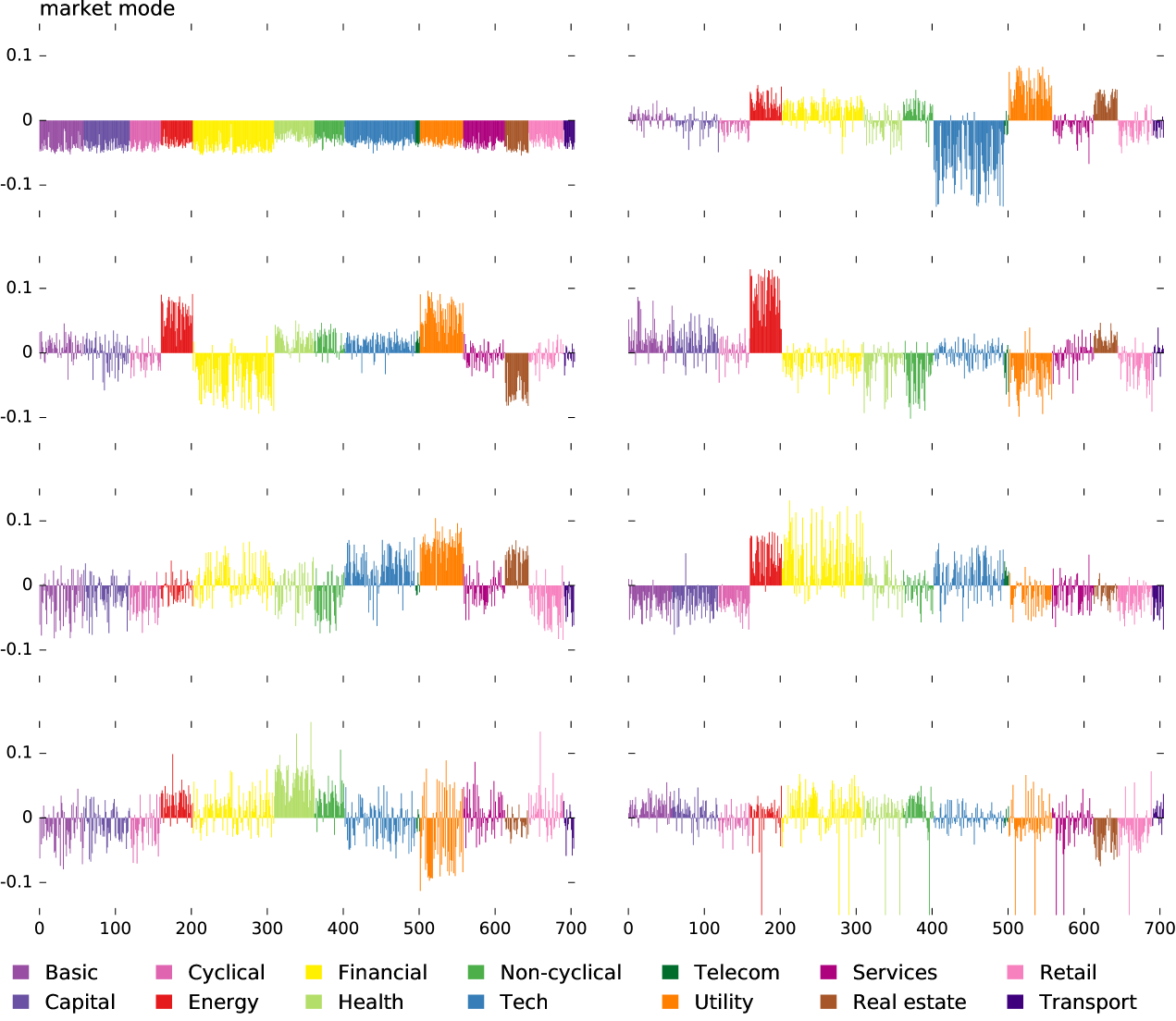
Columns of are the emergent sector time series (basis vectors) representing the corners of the hyper-tetrahedron, and are the participation weights () in sector so that for each stock . The sector matrix is within the convex hull (, ) of the data . It can be found by either minimizing the squared error with convex constraints in factorization as originally proposed (Cutler and Breiman, 1994), or by making a convex hull of the dataset and choosing one or more of its vertices to be basis vectors, or by making a convex hull in low-dimensions and choosing one or more of its vertices to be basis vectors (Thurau et al., 2009), or by minimizing after initializing with candidate archetypes that are guaranteed to lie in the minimal convex set of the data (Mörup and Hansen, 2012). The columns of the matrix are shown in Fig. 6.
Appendix C Calculations and Convergence
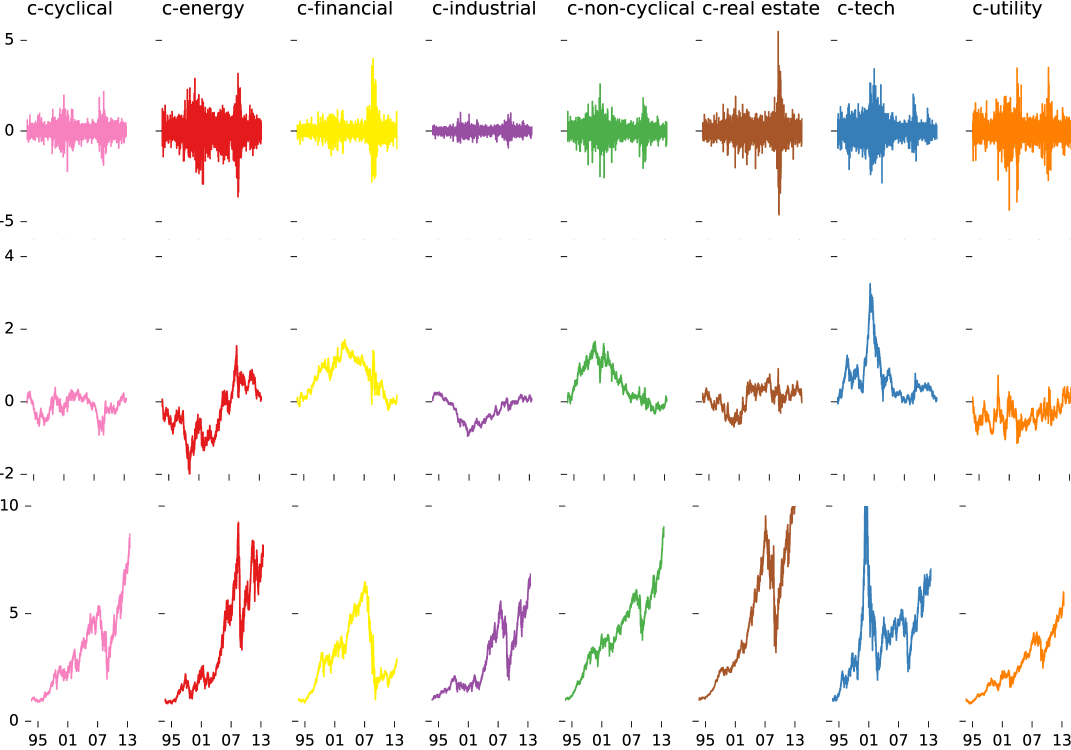
Numerical computations were performed using an in-house Python language implementation of the principal convex hull analysis (PCHA) algorithm as described in (Mörup and Hansen, 2012). For the full dataset, the factorization , with as defined in Eqn. 1 converged in 35 iterations to a predefined tolerance value of , where is the average difference in the sum of squared error per matrix element in from one iteration to the next. The resulting columns of are shown in Fig. 7 (top row). Annualized cumulative log returns are obtained by summing rows of :
| (2) |
The time series are shown in Fig. 3 and the middle row of Fig. 7. Weights for selected stocks are shown in Fig. 2, the remainder are available on the companion website (Chachra et al., 2013). In each canonical sector , the component of weights for companies are shown in Fig. 8.
The analysis of evolving sector weights was performed similarly, but with a sliding Gaussian time window. We decomposed the local normalized log returns for each stock into the canonical sectors determined from the entire time series. Each column (time series) of the returns matrix was multiplied with a Gaussian, of standard deviation centered at to obtain . We use found using the full dataset (Eqn. 1) (corresponding to keeping the sector-defining simplex corners fixed). is factorized to obtain new weights that describe sector decomposition of stocks in that period focused at : . is increased in steps of 50 starting at and ending at , and is calculated at each with the corresponding . These results are plotted in Fig. 5 for a select group of companies; the remainder are available on the companion website (Chachra et al., 2013).
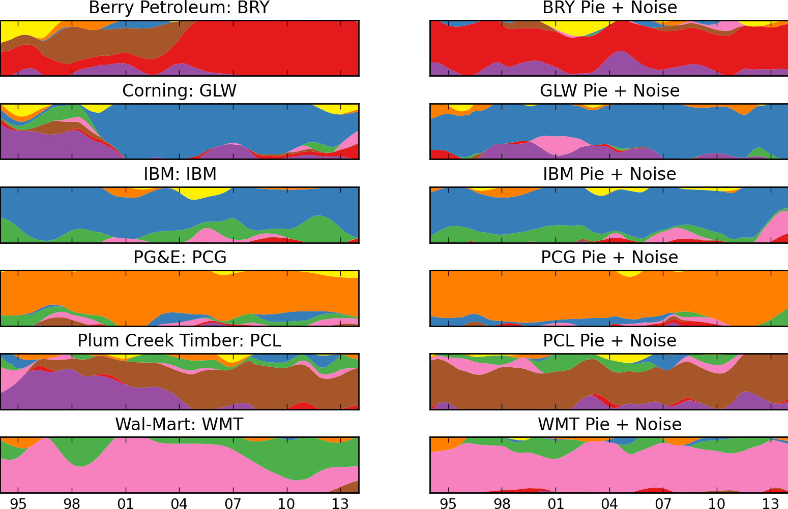
To address the challenge of distinguishing signal from noise in the evolving sector weights, we emulated the effect of noise for each of the companies from Fig. 5. For each of these companies, we took its sector weights, , and multiplied by to obtain a time series for the company with weights that are constant in time. We then added gaussian random noise with standard deviation one and replaced these companies by this simulated data. Fig. 9 shows the comparison between the real flows and the simulated constant data with noise added. General features are shown to be signal while small fluctuations are consistent with noise.
Appendix D Dimensionality of the Space of Price Returns
It is often the case with large datasets that the effective dimensionality of the data space is much lower when one filters out the noise. Of the many dimensional reduction methods, the most commonly used is singular value decomposition (SVD) (Press et al., 2007), a deterministic matrix factorization. We discuss SVD in more detail in order to draw a contrast with previous SVD results, and to apply it for quantifying the explainable variation in the returns data.
An SVD of is a matrix factorization (Press et al., 2007) such that matrices and are orthogonal; is a diagonal matrix of “singular values”. If the goal were purely rank-reduction, entries of chosen to lie above “noise threshold” are retained and the rest truncated so that . This effectively reduces the dimension of to . The choice of can be informed by the distribution of singular values as discussed later. The rows of are precisely the eigenvectors of the stock-stock returns correlation matrix, . It was previously reported that some components of the stiff eigenvectors of this stock-stock correlation matrix loosely corresponded to firms belonging to the same conventionally identified business sector (Plerou et al., 2002) (but see Fig. 10).
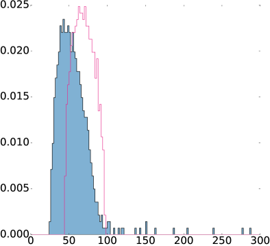
After normalizing the log returns, the returns matrix has entries of unit variance. If the entries were uncorrelated random variables drawn from a standard normal distribution, their singular values (which are also the positive square roots of the eigenvalues of ) would be described by Wishart statistics (Mehta, 2004). The Wishart ensemble for a matrix of size predicts a distribution of singular values with a characteristic shape (Mehta, 2004), bounded for large matrices by . Comparing the stock correlations with Wishart statistics has been previously used to filter noise from financial datasets (Laloux et al., 1999). As shown in Fig. 11, most singular values of the returns matrix lie in the bulk below the bound set by the Wishart ensemble, whereas only 20 fall outside that cutoff (The singular value bounds of a random Gaussian rectangular matrix of size can be shown to be for large matrices.) Historically, this has served as indication that singular values within the bulk correspond to noise (Laloux et al., 1999). Recently, however, much progress has been made in the development of techniques to extract signal from the bulk (Burda et al., 2004, 2006; Livan et al., 2011). Our method does not claim to capture this information. Rather, we measure its ability to capture variation in the data above the cutoff by means of random matrix theory explainable variation as defined in section F. The largest singular value of corresponds to what we will refer to as the “market mode” as this represents overall simultaneous rise and fall of stocks. In the analysis presented in this paper, this mode has been filtered from the returns matrix by projecting the matrix into the subspace spanned by all non-market mode eigenvectors. This is nearly equivalent to filtering the market mode using simple linear regression (as done commonly (Plerou et al., 2002)), although more convenient.
Appendix E Low-Dimensional Projections of Price Returns
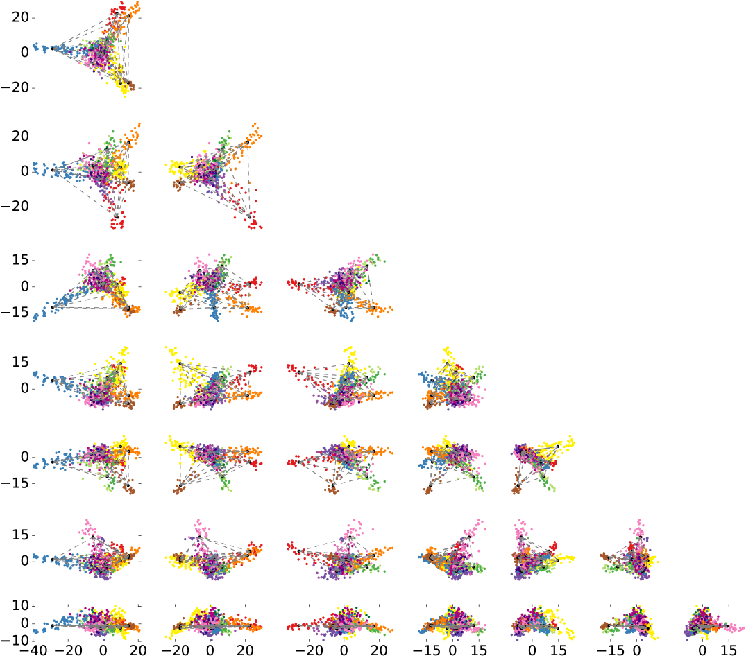
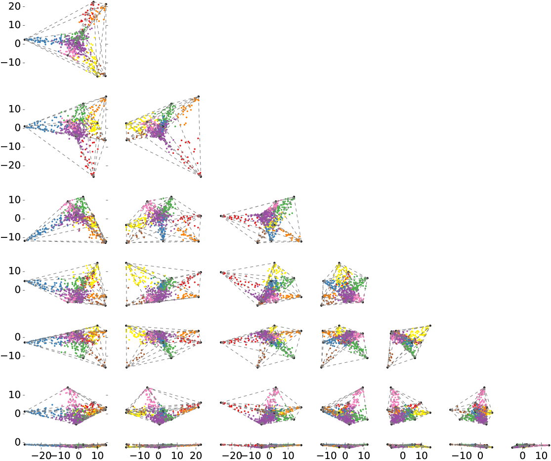
The emergent low-dimensional, hyper-tetrahedral (simplex) structure of stock price returns can be seen by projecting the dataset into stiff “eigenplanes”. Eigenplanes are formed by pairs of right singular vectors from a SVD. Here, we construct an SVD of the simplex corners, ; simplex corners are mapped to columns of because (in other words, is a projection operator). The plots in Fig. 12 are the projections of the dataset, . The rows of taken in pairs form the axes of the projections in Fig. 1 and Fig. 12. With those plots, it becomes clear that the eigenplanes represent projections of a simplex-like data into two-dimensions. Secondly, we note that the simplex structure becomes less clear as one looks at planes corresponding to smaller singular value directions; the signal eventually becomes buried in the noise.
Similarly, the results of the factorization can be seen in eigenplanes from the SVD of . These results (rows of ) are shown in Fig. 13, where we notice that the data is now perfectly resides in simplex region as expected due to constraints.
Appendix F Coefficient of determination ()
We measured the goodness of the returns decomposition by measuring the coefficient of determination () as follows:
| (3) |
Here, SSE denotes the sum of square errors ,
and SST is the total sum of squares . This is also known as the
proportion of variance explained (PVE). For the factorization of the
full dataset, normalized with the market mode removed, the calculated value is
. The SVD of with singular values shown in Fig. 11 provides a convenient way to put this number in context for the returns dataset. Only 20 singular values (excluding the market mode) were above the cut-off that was predicted by random matrix theory for a matrix of purely random Gaussian entries. For any matrix with elements , the norm , where are the singular
values (Press et al., 2007). Thus, the fraction of intrinsic variation in above the cutoff is the sum of squares of the 20 singular values (not including market mode) divided by SST, . Therefore, as a first approximation, the factorization explains
of the random matrix theory (RMT) explainable variation.
| Bulk Variation | 80.2% |
|---|---|
| Explainable Variation | 19.8% |
| Factors | Percent of Explainable Variation |
| Market Mode (MM) | 8.0% |
| 2 factors + MM | 26.0% |
| 3 factors + MM | 36.1% |
| 4 factors + MM | 42.8% |
| 5 factors + MM | 48.9% |
| 6 factors + MM | 55.3% |
| 7 factors + MM | 59.4% |
| 8 factors + MM | 63.7% |
| 9 factors + MM | 68.1% |
| Fama and French | 24.0% |
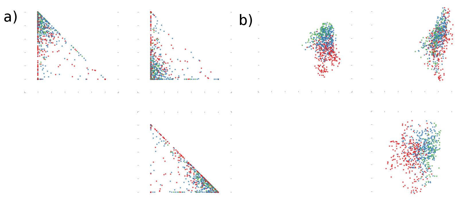
For reference we provide the RMT explainable variation for the factor decomposition of Fama and French, the classification by Scottrade®, and the top 8 singular vectors given by SVD. The percentage of the RMT explainable variation for different numbers of factors compared to the 3 factor decomposition of Fama and French is shown in Table 2. Fama and French have the benefit of allowing factors to have positive or negative weights. In order to compare with another non-negative decomposition, we fix the weight matrix according to the Scottrade® labels and run archetypal analysis for this factor version. The value for this decomposition is with a corresponding RMT explainable variance of compared to for our 8 factors. For completeness, we also note that if is rank-reduced to the eight stiffest components found by SVD (not including market mode), then the factorization explains of the the RMT explainable variation in with overall results in good accord with the analysis presented here. This implies that sector decomposition information was already contained in the stiff modes from the SVD of , however SVD is not the appropriate tool for the decomposition. Fig. 14 further shows that our unsupervised 3-factor decomposition appears quite distinct from Fama and French’s hand-created one.
Appendix G The Number of Canonical Sectors
It is an open problem to determine the effective dimensionality (optimal rank) of a general dataset (matrix). One could select among models of different dimensions using statistical tests such as the discussed above, or information theory based criteria such as Akaike Information Criterion (AIC) or the Bayesian Information Criterion (BIC), but the choice of the selection criterion is itself generally made on an ad hoc basis. Therefore, a direct observation of the comprehensibility of results is often the most reliable criterion. In the dataset used for analysis described here, a factorization with yielded results where both the emergent time series and weights in showed qualitative signs of overfitting. For example, with the results were in good agreement with except for an additional resulting sector involving participation from only 11 seemingly unrelated stocks (Table 3 and Fig. 4). The high-level results of factorization with different values of may be explored in a number of ways, several of which are described below.
| Ticker | Company Name | Label |
|---|---|---|
| EQT | EQT Corporation | Energy |
| RDN | Radian Group Inc. | Financials |
| STT | State Street Corporation | Financials |
| LH | Laboratory Corp. of America Holdings | Healthcare |
| UHS | Universal Health Services Inc. | Healthcare |
| STZ | Constellation Brands Inc. | Non-Cyclicals |
| CNL | Cleco Corporation | Utilities |
| OKE | ONEOK Inc. | Utilities |
| CAKE | The Cheesecake Factory Incorporated | Cyclicals |
| EFX | Equifax Inc. | Industrials |
| ESRX | Express Scripts Holding Company | Non-Cyclicals |
G.1 Sector Changes with Dimensionality
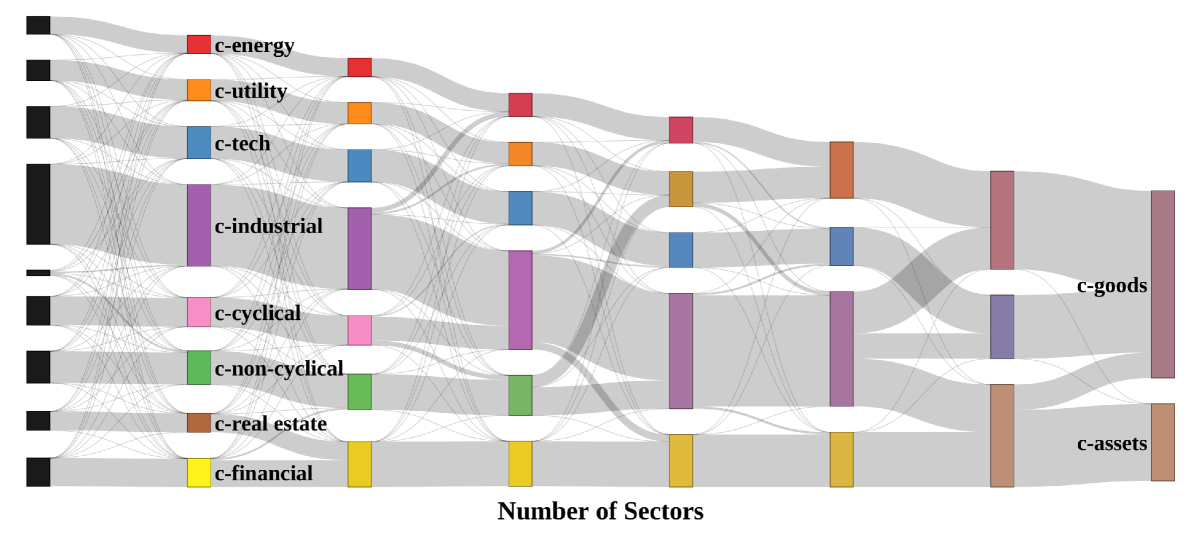
One approach to investigating how the sector decomposition changes with dimension is to produce a flow diagram. To do this, we performed the fit with the constraint . Hence the sectors for can be expressed as a linear combination of sectors for , as a linear combination of , and so forth. The results of these fits are presented in Fig. 5. The figure represents these relationships though connections between the decompositions for and weighted according to the matrix . More precisely, we create a node corresponding to each of the 9 sectors whose size is proportional to where is the weight matrix for the 9 sector decomposition. Hence, the relative node sizes represent the amount of the market particpating in the sector. Multiplying this vector by gives the approximate size for each node in . Multiplying this vector by gives the approximate size for each node in , and so on. In this way, we generate a Sankey diagram whose node sizes correspond roughly to the amount of the market in the sector and whose connections depict how strongly the sectors for decompositions with different overlap. In the image, we see that the decomposition gives the 8 sector version with an additional small sector whose companies were listed in Table 3. We also see that for c-finance and c-real estate merge. At , c-industrial and c-cyclical merge. For , the new sector containing c-industrial and c-cyclical merges with c-non-cyclical. For , c-utility and c-energy merge. Finally, for and , no clear pattern emerges given this image alone.
G.2 Two and Three Sector Decompositions
| c-assets | label | percent | full name | c-goods | label | percent | full name |
|---|---|---|---|---|---|---|---|
| DDR | real estate | 1.77% | DDR Corp. | HON | tech | 0.53% | Honeywell International Inc. |
| ONB | financial | 1.7% | Old National Bankcorp. | TMO | health | 0.51% | Thermo Fisher Scientific Inc. |
| BRE | real estate | 1.66% | Brookfield Real Estate Serv. | NAV | cyclical | 0.49% | Navistar International Corp. |
| PEI | real estate | 1.54% | Pennsylvania RIT | CSL | basic | 0.47% | Carlisle Companies Inc. |
| FMBI | financial | 1.5% | First Midwest Bancorp. Inc. | IRF | tech | 0.47% | International Rectifier Corp. |
| PRK | financial | 1.5% | Park National Corp. | APD | basic | 0.46% | Air Products & Chemicals Inc. |
| BAC | financial | 1.42% | Bank of America Corp. | PCP | basic | 0.43% | Precision Castparts Corp. |
| STI | financial | 1.41% | SunTrust Banks Inc. | OMC | misc services | 0.43% | Omnicom Group Inc. |
| DRE | real estate | 1.29% | Duke Realty Corp. | MXIM | tech | 0.43% | Maxim Integrated Products, Inc. |
| UBSI | financial | 1.28% | United Bankshares Inc. | TFX | health | 0.41% | Teleflex Inc. |
| CPT | real estate | 1.28% | Camden Property Trust | NSC | transport | 0.41% | Norfolk Southern Corp. |
| PPS | real estate | 1.28% | Post Properties Inc. | NBL | energy | 0.4% | Noble Energy Inc. |
| WABC | financial | 1.26% | Westamerica Bancorp. | SM | energy | 0.4% | SM Energy Company |
| FMER | financial | 1.26% | FirstMerit Corp. | WMT | retail | 0.39% | Wal-Mart Stores Inc. |
| CNA | financial | 1.26% | CNA Financial Corp. | CR | basic | 0.38% | Crane Co. |
| VLY | financial | 1.25% | Valley National Bancorp. | ADI | tech | 0.38% | Analog Devices Inc. |
| MTB | financial | 1.24% | M&T Bankcorp. | ITW | cyclical | 0.38% | Illinois Tool Works Inc. |
| WRI | real estate | 1.23% | Weingarten Realty Investors | PPG | basic | 0.38% | PPG Industries Inc. |
| BDN | real estate | 1.21% | Brandywine Realty Trust | BA | capital | 0.38% | The Boeing Company |
| ZION | financial | 1.2% | Zions Bancorp. | AME | tech | 0.38% | Ametek Inc. |
| Total | 27.54% | Total | 8.53% |
| sector 1 | label | percent | sector 2 | label | percent | sector 3 | label | percent |
|---|---|---|---|---|---|---|---|---|
| XOM | energy | 1.29% | BRE | real estate | 2.16% | IRF | tech | 1.29% |
| HP | energy | 1.22% | PEI | real estate | 2.08% | EMC | tech | 1.22% |
| CVX | energy | 1.21% | BWS | retail | 1.99% | ADI | tech | 1.21% |
| ETR | utility | 1.2% | CNA | financial | 1.79% | CSCO | tech | 1.2% |
| APD | basic | 1.2% | ONB | financial | 1.73% | TXN | tech | 1.2% |
| OXY | energy | 1.19% | DDR | real estate | 1.63% | BMC | tech | 1.19% |
| NFG | utility | 1.18% | PRK | financial | 1.59% | SNPS | tech | 1.18% |
| PX | basic | 1.17% | CBSH | financial | 1.59% | PLXS | tech | 1.17% |
| CL | non-cyclical | 1.16% | BC | cyclical | 1.56% | CPWR | tech | 1.16% |
| NBL | energy | 1.15% | FMER | financial | 1.55% | AVT | tech | 1.15% |
| OII | energy | 1.11% | RDN | financial | 1.54% | SWKS | tech | 1.11% |
| LNT | utility | 1.11% | MAS | capital | 1.54% | HPQ | tech | 1.11% |
| D | utility | 1.08% | DDS | retail | 1.47% | PMCS | tech | 1.08% |
| DTE | utility | 1.07% | FMBI | financial | 1.47% | MXIM | tech | 1.07% |
| SCG | utility | 1.06% | ALK | transport | 1.46% | ARW | tech | 1.06% |
| WEC | utility | 1.04% | WABC | financial | 1.43% | TER | tech | 1.04% |
| APA | energy | 0.99% | PCH | real estate | 1.42% | ATML | tech | 0.99% |
| BAX | health | 0.98% | VLY | financial | 1.41% | MCHP | tech | 0.98% |
| MUR | energy | 0.98% | BAC | financial | 1.41% | LRCX | tech | 0.98% |
| CPB | non-cyclical | 0.98% | STI | financial | 1.37% | CGNX | tech | 0.98% |
| Total | 22.38% | Total | 19.14% | Total | 32.18% |
| sector 1 | full name | sector 2 | full name | sector 3 | full name |
|---|---|---|---|---|---|
| XOM | Exxon Mobil Corp. | BRE | Brookfield Real Estate Serv. | IRF | International Rectifier Corp. |
| HP | Helmerich & Payne Inc. | PEI | Pennsylvania RIT | EMC | EMC Corp. |
| CVX | Chevron Corp. | BWS | Brown Shoe Co. Inc. | ADI | Analog Devices Inc. |
| ETR | Entergy Corp. | CNA | CNA Financial Corp. | CSCO | Cisco Systems Inc. |
| APD | Air Products & Chemicals Inc. | ONB | Old National Bancorp. | TXN | Texas Instruments Inc. |
| OXY | Occidental Petroleum | DDR | DDR Corp. | BMC | BMC Software Inc. |
| NFG | National Fuel Gas Company | PRK | Park National Corp. | SNPS | Synopsys Inc. |
| PX | Praxair Inc. | CBSH | Commerce Bancshares Inc. | PLXS | Plexus Corp. |
| CL | Colgate-Palmolive Co. | BC | Brunswick Corp. | CPWR | Compuware Corp. |
| NBL | Noble Energy Inc. | FMER | FirstMerit Corp. | AVT | Avnet Inc. |
| OII | Oceaneering International Inc. | RDN | Radian Group Inc. | SWKS | Skyworks Solutions Inc. |
| LNT | Alliant ENergy Corp. | MAS | Masco Corp. | HPQ | Hewlett-Packard Company |
| D | Dominion Resources Inc. | DDS | Dillard’s Inc. | PMCS | PMC-Sierra Inc. |
| DTE | DTE Energy Corp. | FMBI | First Midwest Bancorp. Inc. | MXIM | Maxim Integrated Products Inc. |
| SCG | SCANA Corp. | ALK | Alaska Air Group Inc. | ARW | Arrow Electronics Inc. |
| WEC | Wisconsin Energy Corp. | WABC | Westamerica Bancorp. | TER | Teradyne Inc. |
| APA | Apache Corp. | PCH | Potlatch Corp. | ATML | Atmel Corp. |
| BAX | Baxter International Inc. | VLY | Valley National Bancorp. | MCHP | Microchip Technology Inc. |
| MUR | Murphy Oil Corp. | BAC | Bank of America Corp. | LRCX | Lam Research Corp. |
| CPB | Campbell Soup Company | STI | SunTrust Banks Inc. | CGNX | Cognex Corp. |
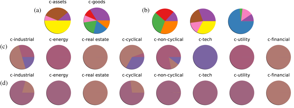
We further explore the two and three sector decompositions by examining their constituent companies and looking at pie charts describing the relationship between our 8 sector decomposition and those with and respectively. Recall that each archetype is constrained to be a linear combination of companies, or in other words to lie in the convex hull of the data. Using this information, we list the 20 companies which contribute the most to each sector in the two and three factor decompositions (Tables 4, 5 and 6). For the two sector decomposition, we find the sectors divide roughly into c-assets (e.g. financial and real estate companies) and c-goods (e.g. companies which provide goods and services). For , the division is less clear. Another way to look at the constituents of these sectors is by examining pie chart representations of these decompositions. Again consider the fit with the constraint . Applying this, we can express the two sector archetypes as linear combinations of the 8 sector archetypes and vice versa. Additionally, we can do the same for the three factor decomposition. The pie charts these fits produce are shown in Fig. 15. The results are consistent with the sector breakdowns described from examining the constituent companies.
G.3 Robustness
In general, a factorization analysis of the returns dataset would be sensitive to number of stocks in the dataset, criteria applied for picking stocks, period over which historical prices are obtained, and frequency at which returns are computed. A robust macroeconomic analysis would therefore require a large number of stocks chosen without sampling bias, with returns calculated over the period of interest and sensitivity checked for frequency of returns calculation. On the other hand, an equity fund manager faces a less daunting task for an analysis that is limited to the universe of her portfolio of stocks: either to find its canonical sectors, or to analyse the exposure of her holdings to the core sectors of the economy.
Appendix H Canonical Sector Indices
The matrix in decomposition represents how returns of stocks must be combined to make canonical sector returns . Since a canonical sector is defined as a combination of stocks, an investment in the sector can made via buying a basket of constituent stocks in proportions given by or through an index :
| (4) |
where, are stocks prices suitably weighted by market cap or other divisor as common practice for common indices (Tagiliani, 2009). An unweighted index of this kind is shown in the bottom row of Fig. 7 for results corresponding to the analysis described in this paper. Conversely, a pre-defined basket of stocks such as the S&P 500® can be unbundled to find its exposure to the canonical sectors. With an investment strategy employing longs and shorts at the same time in correct proportions, it is conceivable to invest in, for example, the c-tech component of S&P 500®.
The desirable features of an index include completeness, objectivity and investability (Pastor et al., 2013). The c-indices constructed using the ideas outlined here would not only be of value to investors through investment vehicles such as ETFs, Futures, etc., but also serve as important economic indicators.
References
- Basalto et al. (2005) Basalto, N., Bellotti, R., Carlo, F.D., Facchi, P. and Pascazio, S., Clustering stock market companies via chaotic map synchronization. Physica A: Statistical Mechanics and its Applications, 2005, 345, 196 – 206.
- Berry Petroleum Company History (2013) Berry Petroleum Company History, , 2013. Available online at: http://www.bry.com/pages/history.html (accessed 2015-01-01).
- Bonanno et al. (2003) Bonanno, G., Caldarelli, G., Lillo, F. and Mantegna, R.N., Topology of correlation-based minimal spanning trees in real and model markets. Phys. Rev. E, 2003, 68, 046130.
- Bonanno et al. (2000) Bonanno, G., Vandewalle, N. and Mantegna, R.N., Taxonomy of stock market indices. Phys. Rev. E, 2000, 62, R7615–R7618.
- Bostock et al. (2011) Bostock, M., Ogievetsky, V. and Heer, J., D3: Data-Driven Documents. IEEE Trans. Visualization & Comp. Graphics (Proc. InfoVis), 2011.
- Burda et al. (2004) Burda, Z., Görlich, A., Jarosz, A. and Jurkiewicz, J., Physica A, 2004, 343.
- Burda et al. (2006) Burda, Z., Görlich, A., Jurkiewicz, J. and Wacław, B., Eur. Phys. J. B, 2006, 49.
- Bury (2013) Bury, T., Market structure explained by pairwise interactions. Physica A: Statistical Mechanics and its Applications, 2013, 392, 1375 – 1385.
- CBOE® Oil Index (2013) CBOE® Oil Index, , 2013. Available online at: http://www.cboe.com/products/IndexComponentsAuto.aspx?PRODUCT=OIX (accessed 2015-01-01).
- Chachra et al. (2013) Chachra, R., Alemi, A.A., Hayden, L., Ginsparg, P.H. and Sethna, J.P., Project Website with additional figures and analyses [online]. , 2013. Available online at: www.lassp.cornell.edu/sethna/Finance (accessed 2015-01-01).
- Conlon et al. (2009) Conlon, T., Ruskin, H. and Crane, M., Cross-correlation dynamics in financial time series. Physica A: Statistical Mechanics and its Applications, 2009, 388, 705 – 714.
- Conversano and Vistocco (2010) Conversano, C. and Vistocco, D., Analysis of mutual funds’ management styles: a modeling, ranking and visualizing approach. Journal of Applied Statistics, 2010, 37, 1825–1845.
- Coronnello et al. (2005) Coronnello, C., Tumminello, M., Lillo, F., Micciche, S. and Mantegna, R., Sector identification in a set of stock return time series traded at the London Stock Exchange. Acta Physica Polonica B, 2005, 36, 2653–2679.
- Cutler and Breiman (1994) Cutler, A. and Breiman, L., Archetypal Analysis. Technometrics, 1994, 36, 338–347.
- Ding and He (2004) Ding, C. and He, X., K-means Clustering via Principal Component Analysis. In Proceedings of the Proceedings of the Twenty-first International Conference on Machine Learning, ICML ’04, Banff, Alberta, Canada, pp. 29–, 2004 (ACM: New York, NY, USA).
- Ding et al. (2010) Ding, C.H.Q., Li, T. and Jordan, M.I., Convex and Semi-Nonnegative Matrix Factorizations. IEEE Trans. Pattern Anal. Mach. Intell., 2010, 32, 45–55.
- Dow Jones® US Indices: Industry Indices (2015) Dow Jones® US Indices: Industry Indices, , 2015. Available online at: www.djindexes.com/mdsidx/downloads/fact_info/Dow_Jones_US_Indices_Industry_Indices_Fact_Sheet.pdf (accessed 2015-01-01).
- Doyle and Elkan (2009) Doyle, G. and Elkan, C., Financial Topic Models. In Proceedings of the NIPS Workshop on Applications for Topic Models: Text and Beyond, 2009 (Whistler, Canada).
- Eom et al. (2007) Eom, C., Oh, G., Jeong, H. and Kim, S., Topological Properties of Stock Networks Based on Random Matrix Theory in Financial Time Series. Papers, arXiv.org, 2007.
- Fama and French (1993) Fama, E.F. and French, K.R., Common risk factors in the returns on stocks and bonds. Journal of financial economics, 1993, 33, 3–56.
- Fenn et al. (2011) Fenn, D.J., Porter, M.A., Williams, S., McDonald, M., Johnson, N.F. and Jones, N.S., Temporal evolution of financial-market correlations. Phys. Rev. E, 2011, 84, 026109.
- Heimo et al. (2009) Heimo, T., Kaski, K. and Saramäki, J., Maximal spanning trees, asset graphs and random matrix denoising in the analysis of dynamics of financial networks. Physica A: Statistical Mechanics and its Applications, 2009, 388, 145 – 156.
- Hyvärinen and Oja (2000) Hyvärinen, A. and Oja, E., Independent Component Analysis: Algorithms and Applications. Neural Netw., 2000, 13, 411–430.
- Kersting et al. (2010) Kersting, K., Wahabzada, M., Thurau, C. and Bauckhage, C., Hierarchical Convex NMF for Clustering Massive Data.. Journal of Machine Learning Research - Proceedings Track, 2010, 13, 253–268.
- Kim and Jeong (2005) Kim, D.H. and Jeong, H., Systematic analysis of group identification in stock markets. Phys. Rev. E, 2005, 72, 046133.
- Kullmann et al. (2000) Kullmann, L., Kertész, J. and Mantegna, R.N., Identification of clusters of companies in stock indices via Potts super-paramagnetic transitions. Physica A: Statistical Mechanics and its Applications, 2000, 287, 412–419.
- Laloux et al. (1999) Laloux, L., Cizeau, P., Bouchaud, J.P. and Potters, M., Noise Dressing of Financial Correlation Matrices. Phys. Rev. Lett., 1999, 83, 1467–1470.
- Lee and Seung (1999) Lee, D.D. and Seung, H.S., Learning the parts of objects by non-negative matrix factorization. Nature, 1999, 401, 788–791.
- Li and Ding (2006) Li, T. and Ding, C., The Relationships Among Various Nonnegative Matrix Factorization Methods for Clustering. Data Mining, 2006. ICDM ’06. Sixth International Conference on, 2006, pp. 362–371.
- Livan et al. (2011) Livan, G., Alfarano, S. and Scalas, E., Phys. Rev. E, 2011, 84.
- Mantegna (1999) Mantegna, R.N., Hierarchical structure in financial markets. The European Physical Journal B - Condensed Matter and Complex Systems, 1999, 11, 193–197.
- Martins (2007) Martins, A.C., Random, but not so much a parameterization for the returns and correlation matrix of financial time series. Physica A: Statistical Mechanics and its Applications, 2007, 383, 527 – 532.
- Mehta (2004) Mehta, M.L., Random Matrices, 3 , 2004 (Academic Press: Boston, MA, USA).
- Morgan Stanley® High-Tech 35 Index (2005) Morgan Stanley® High-Tech 35 Index, , 2005. Available online at: www.nasdaq.com/options/indexes/msh.aspx (accessed 2015-01-01).
- Mörup and Hansen (2012) Mörup, M. and Hansen, L.K., Archetypal analysis for machine learning and data mining. Neurocomputing, 2012, 80, 54 – 63.
- Musmeci et al. (2014) Musmeci, N., Aste, T. and Di Matteo, T., Relation between Financial Market Structure and the Real Economy: Comparison between Clustering Methods. SSRN, 2014.
- Nadig and Crigger (2011) Nadig, D. and Crigger, L., Signal From Noise. Journal of Indexes, 2011, 14, 40–43, 50.
- Pastor et al. (2013) Pastor, L., Heaton, J. and Foss, A., The index is dead. Long Live the Index. Journal of Indexes, 2013, 16, 16–21, 55.
- Plerou et al. (2002) Plerou, V., Gopikrishnan, P., Rosenow, B., Amaral, L.A.N., Guhr, T. and Stanley, H.E., Random matrix approach to cross correlations in financial data. Phys. Rev. E, 2002, 65, 066126.
- Plum Creek® History (2014) Plum Creek® History, , 2014. Available online at: http://www.plumcreek.com/AboutPlumCreek/History/tabid/55/Default.aspx (accessed 2015-01-01).
- Podobnik and Stanley (2008) Podobnik, B. and Stanley, H.E., Detrended Cross-Correlation Analysis: A New Method for Analyzing Two Nonstationary Time Series. Phys. Rev. Lett., 2008, 100, 084102.
- Press et al. (2007) Press, W.H., Teukolsky, S.A., Vetterling, W.T. and Flannery, B.P., Numerical Recipes 3rd Edition: The Art of Scientific Computing, 3 , 2007 (Cambridge University Press: New York, NY, USA).
- Russell 3000® Index (2015) Russell 3000® Index, , 2015. Available online at: www.russell.com/indexes/data/fact_sheets/us/russell_3000_index.asp (accessed 2015-01-01).
- Scottrade® (2015) Scottrade®, , 2015. Available online at: www.scottrade.com (accessed 2015-01-01).
- S&P 500® Index (2014) S&P 500® Index, , 2014. Available online at: us.spindices.com/indices/equity/sp-500 (accessed 2015-01-01).
- Tagiliani (2009) Tagiliani, M., The Practical Guide to Wall Street, 1 , 2009 (John Wiley & Songs, Inc.: Hoboken, NJ, USA).
- Thurau et al. (2009) Thurau, C., Kersting, K. and Bauckhage, C., Convex Non-negative Matrix Factorization in the Wild. In Proceedings of the Data Mining, 2009. ICDM ’09. Ninth IEEE International Conference on, pp. 523–532, 2009.
- Thurau et al. (2010) Thurau, C., Kersting, K. and Bauckhage, C., Yes We Can—simplex volume maximization for descriptive web scale matrix factorization.. In Proceedings of the CIKM, edited by J. Huang, N. Koudas, G.J.F. Jones, X. Wu, K. Collins-Thompson and A. An, pp. 1785–1788, 2010, ACM.
- Thurau et al. (2011) Thurau, C., Kersting, K., Wahabzada, M. and Bauckhage, C., Convex non-negative matrix factorization for massive datasets. Knowledge and Information Systems, 2011, 29, 457–478.
- Tsalmantza and Hogg (2012) Tsalmantza, P. and Hogg, D.W., A Data-driven Model for Spectra: Finding Double Redshifts in the Sloan Digital Sky Survey. The Astrophysical Journal, 2012, 753, 122.
- Vistocco and Conversano (2009) Vistocco, D. and Conversano, C., Visualizing and clustering financial portfolios using internal compositions. SIS, 2009 Presented at Statistical Methods for the Analysis of Large Data-Sets Pescara, Italy, September 23-25, http://new.sis-statistica.org/wp-content/uploads/2013/10/CO09-Visualizing-and-clustering-financial-portfolios-using.pdf.
- Wang and Zhang (2013) Wang, Y.X. and Zhang, Y.J., Nonnegative Matrix Factorization: A Comprehensive Review. Knowledge and Data Engineering, IEEE Transactions on, 2013, 25, 1336–1353.
- Yahoo!® Finance (2015) Yahoo!® Finance, , 2015. Available online at: finance.yahoo.com (accessed 2015-01-01).
- Zhang et al. (2007) Zhang, Z., Li, T., Ding, C. and Zhang, X., Binary Matrix Factorization with Applications. In Proceedings of the Proceedings of the 2007 Seventh IEEE International Conference on Data Mining, ICDM ’07, pp. 391–400, 2007 (IEEE Computer Society: Washington, DC, USA).