Capturing Polytopal Symmetries by Coloring the Edge-Graph
Abstract.
A general (convex) polytope and its edge-graph can have very distinct symmetry properties. We construct a coloring (of the vertices and edges) of the edge-graph so that the combinatorial symmetry group of the colored edge-graph is isomorphic (in a natural way) to , the group of linear symmetries of the polytope. We also construct an analogous coloring for , the group of orthogonal symmetries of .
Key words and phrases:
convex polytopes, linear symmetries, orthogonal symmetries, edge-graph, graph coloring, graph symmetries2010 Mathematics Subject Classification:
51M20, 52B05, 52B11, 52B15, 05C501. Introduction
In the context of this article, a polytope will always be a convex polytope, that is, is the convex hull of finitely many points. A symmetry of is a certain transformation of the ambient space that fixes the polytope set-wise. Our focus is specifically on the groups
called the linear resp. orthogonal symmetry group of .
Initially defined geometrically, one can ask whether it is possible to understand these symmetry groups combinatorially. This could mean to identify a purely combinatorial object whose combinatorial symmetry group is isomorphic to resp. in a natural way.
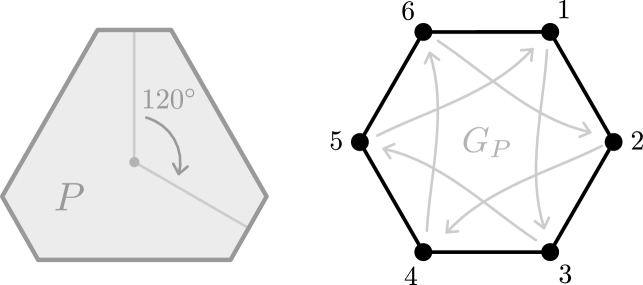
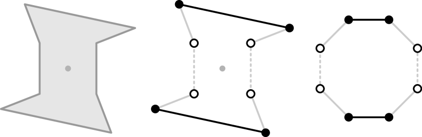
For example, consider the edge-graph of the polytope. Every, say, linear symmetry induces a distinct combinatorial symmetry of the edge-graph (see Figure˜1). We could state this as follows: the edge-graph is at least as symmetric as the polytope. Usually however, it is strictly more symmetric and is therefore unsuited for “capturing the polytope’s symmetries” in our sense.
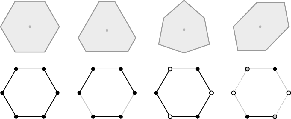
In this article we ask whether this can be fixed by coloring the vertices and edges of the edge-graph, thereby encoding further geometric information, and hopefully creating a combinatorial objects that is exactly as symmetric as (see Figure˜2). As we shall see, this is indeed possible.
This should be surprising for at least two reasons. First, it is established wisdom that the edge-graph of a general polytope in dimension carries only very little information about the polytope (a graph can be the edge-graph of several combinatorially distinct polytopes, potentially of different dimensions). Thus, whether the geometric symmetries of can be captured by coloring only the edges and vertices of (instead of, say, also higher dimensional faces) should be at least controversial. Second, the same statement is actually wrong for more general geometric objects (such as graph embeddings, see Example˜6.5). In fact, our proof for the existence of these colorings is based on a construction by Ivan Izmestiev [4], which relies heavily on the convexity of . Because of this, it is unclear whether our result generalizes to even some form of non-convex polytopes or polytopal complexes.
Our investigation is in part motivated from a result by Bremner et al. [3]: given a polytope with vertices, the authors construct a coloring of the complete graph , so that the symmetry group of the colored graph is isomorphic to (resp. ; a more precise statement is given in Section˜2.1). We can interpret this as follows: if we are allowed to color not only the vertices and edges of , but also other pairs of vertices without a direct counterpart in the polytope’s combinatorics, then “capturing the polytope’s symmetries” is indeed possible. The major result of our article is then that coloring these “non-geometric edges” is not actually necessary.
We reiterate this introduction in a more formal manner.
1.1. Notation and setting
Throughout the text we let denote a convex polytope that is full-dimensional (i.e., not contained in any proper affine subspace of ) and contains the origin in its interior (i.e., ).
By we denote the set of -dimensional faces of . We assume a fixed enumeration of the polytope’s vertices. In particular, will always denote the number of the vertices.
The edge-graph of is the finite simple graph with vertex set and edge set . We implicitly assume that corresponds to the vertex , and that (short for ) if and only if .
The (combinatorial) symmetry group of 111For convenience, notions like the symmetry group, colorings, the adjacency matrix, etc. are only introduced for the edge-graph, but it is understood that they apply to more general graphs as well. is defined as
that is, the group of permutations of that fix the edge set of .
A coloring of is a map (it assign colors to both, vertices and edges), where denotes an abstract set of colors. The pair is then a colored edge-graph and will be abbreviated by . Its combinatorial symmetry group is
If , we also say that preserves the coloring .
The colored adjacency matrix of is the matrix with entries
Clearly, a coloring is completely determined by the colored adjacency matrix, and we might occasionally use to define a coloring.
A geometric symmetry of maps vertices of onto vertices of and thus describes a permutation of the vertex set. Let be the permutation of the vertex set of the edge-graph that permutes its vertices in the same way as permutes the vertices of . Formally, that is
| (1.1) |
Since also maps edges of onto edges of , also maps edges to edges, and so we see that is a symmetry of the edge-graph, i.e., ). The assignment then defines a group homomorphism which we shall call the natural group homomorphism of the polytope .
Since is full-dimensional, its vertices contain a basis of , and it follows that must be injective. In general however, is not an isomorphism and , which is a formal way to say that the edge-graph can have many more symmetries than the polytope.
Our approach for rectifying this is to assign a coloring to the edge-graph with the hope that . The natural candidate for the isomorphism between the groups is a colored version of the natural homomorphism:
| (1.2) |
For this to work as desired, we need to check two things:
-
•
First, needs to be well-defined. This is not the case for each coloring: one needs to check that for each the corresponding permutation is indeed a symmetry of (that is, is in ). Intuitively, this amounts to checking that the edge-graph, even after coloring, is still at least as symmetric as .
-
•
Second, must have an inverse. If so, then is exactly as symmetric as . Providing such an inverse will go as follows: for each we need to construct a geometric symmetry with
Since is full-dimensional, if exists then it is unique. The map is then the desired inverse.
The discussion also applies verbatim to the orthogonal symmetry group , and we shall use the same notation to denote the natural homomorphism in this case.
With this in place, we can formalize “capturing symmetries”:
Definition 1.1.
A coloring of is said to capture the linear (resp. orthogonal) symmetries of if (resp. ), where the isomorphism is realized by the natural homomorphism .
The main results of this article are explicit constructions for colorings that
-
•
capture linear symmetries (Theorem˜4.7).
-
•
capture orthogonal symmetries (Theorem˜5.2).
1.2. Overview
In Section˜2 we introduce the metric coloring and the orbit coloring, two very natural candidates for capturing certain polytopal symmetries. In this section we do not yet show that either coloring capture linear or orthogonal symmetries, but we establish relevant properties used in the upcoming sections.
In Section˜3 we derive a sufficient condition for a coloring of the form (the colors are real numbers) to capture linear symmetries. The criterion will be in terms of the eigenspaces of the (colored) adjacency matrix of the edge-graph. We shall call this the “linear algebra criterion”.
In Section˜4 we introduce the Izmestiev coloring (based on a construction by Ivan Izmestiev [4]) and we show that it satisfies the “linear algebra criterion” from Section˜3. We thereby establish the existence of a first coloring that captures linear symmetries (Theorem˜4.7). As a corollary we find that the orbit coloring captures linear symmetries as well (Corollary˜4.8).
In Section˜5 we show that a combination of the Izmestiev coloring and the metric coloring captures orthogonal symmetries (Theorem˜5.2).
2. Two useful colorings
This section is preliminary, in that it introduce two natural colorings of the edge-graph, the metric coloring and the orbit coloring, without establishing either coloring as capturing polytopal symmetries. In fact, this is an open question for the metric coloring (see ˜6.6). The orbit coloring captures polytopal symmetries, but we are not able to show this right away. Both colorings will play a role in the upcoming sections.
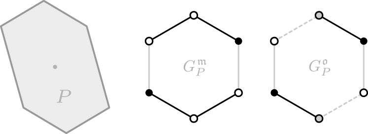
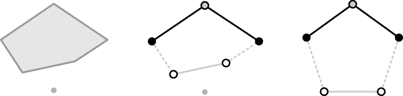
Figure˜3 shows a polygon and its edge-graph with either coloring applied.
2.1. The metric coloring
Our first coloring is motivated from the previously mentioned construction of Bremner et al. [3] – a coloring of the complete graph that “captures orthogonal symmetries”. In our notation their result reads as follows:
Theorem 2.1 ([3, Theorem 2]333This result is primarily based on [2, Proposition 3.1], but we found that its first explicit formulation is in [3] ).
Given a polytope with vertex set . Consider the coloring on the complete graph with
Then .
The strength of this result lies in its immediate applicability: constructing this “complete metric coloring” requires no knowledge of the edge-graph (which is usually hard to come by), but only the vertex coordinates of 444If is given in -representation, one can apply Theorem 2.1 to compute the orthogonal symmetry group of the dual polytope , which is identical to as a matrix group.. In practice, this is probably the best tool for an explicit computation of .
From a theoretical and aesthetic perspective however, this construction has the flaw of containing massively redundant data and stepping outside the combinatorial structure of the polytope (we assign color to vertex-pairs that are not edges of the polytope). Naturally, we can ask whether one can get away with coloring fewer of these “non-edges”, ideally only the actual edges of the edge-graph.
Based on this hope, we define the following:
Definition 2.2.
The metric coloring of is the coloring 555 A coloring whose colors are real numbers is still a purely combinatorial objects. These numbers are just used for a concise definition and could be replaced by any other finite set of distinguishable values. The only information used from the coloring (in the form of the combinatorial symmetry group of the colored graph) is whether two vertices/edges receive the same or a different color. with
Whether the metric coloring captures orthogonal symmetries is an open question (see also ˜6.6). Our reason for introducing it anyway is that in Section˜5 the metric coloring will be one ingredient to a coloring that indeed captures orthogonal symmetries.
We close this section with another formulation of Theorem˜2.1 that also allows for capturing linear symmetries (in fact, this is closer to the original formulation in [3]). Note that the complete metric coloring of in Theorem˜2.1 can also be described by its colored adjacency matrix , where is the matrix in which the vertex coordinates of appear as columns.
Theorem 2.3 (Another formulation of [3, Theorem 2]).
Let be a coloring of the complete graph with colored adjacency matrix :
-
()
if , then (this is exactly Theorem˜2.1).
-
()
if 666 denotes the Moore-Penrose pseudo inverse of , that is, ., then .
A proof for part (ii) will also follow from the theory developed in Section˜3 (see Remark˜3.2)
2.2. The orbit coloring
The next coloring is motivated from the following consideration: suppose that we are given two vertices in the same orbit w.r.t. , which just means that there is a with . The corresponding combinatorial symmetry satisfies . If now is a coloring that captures linear symmetries, then preserves the coloring and we have . We can summarize this as follows: if is supposed to capture linear symmetries, then vertices in the same -orbit of must have the same color in . With an analogous argument we see that the same holds for edges.
Having identified this first necessary condition for capturing symmetries, we can consider the “simplest” coloring that follows this idea:
Definition 2.4.
The (linear) orbit coloring of assigns the same color to vertices (resp. edges) of if and only if the corresponding vertices (resp. edges) of are in the same -orbit.
An analogous coloring can be defined for orthogonal symmetries, which we shall call the orthogonal orbit coloring of , still denoted by . For the sake of conciseness, this section only discusses the (linear) orbit coloring, but all statements carry over to the orthogonal version in the obvious way.
As we shall learn in Section˜4 (see Corollary˜4.8), the orbit coloring indeed captures linear symmetries. However, this is surprisingly hard to show directly. In fact, our eventual proof of this will “just” use the following:
Lemma 2.5.
If there is any coloring that captures linear symmetries, then so does the orbit coloring .
Proof.
Suppose that is a coloring that captures linear symmetries, in particular, is an isomorphism. Our proof that captures linear symmetries as well is based on two simple observations:
-
()
the natural homomorphism is well-defined (that is, is at least as symmetric as ), and
-
()
.
Showing either is straight-forwarded, but for the sake of completeness, both proofs are included below. Now, presupposing both, we can write down the following chain of groups in which the first and the last group are the same:
Since all maps are injective, and the groups are finite, all maps must actually be isomorphisms. Thus, is an isomorphism and captures linear symmetries. This concludes the proof, and it remains to verify (i) and (ii).
Proof of (i): let be a linear symmetry of with corresponding combinatorial symmetry . We need to show that . For this, we observe that for each the vertices and belong to the same -orbit of . By the definition of the orbit coloring, and have then the same color in . Thus, preserves the vertex colors of . Analogously, one shows that preserves edge colors. Thus, .
Proof of (ii): let be a permutation that preserves the orbit coloring. We need to show . For this, we observe that for all the vertices and have the same color in , which just means (by Definition˜2.4) that are in the same -orbit of . Repeating the argument of the introductory paragraph to this section we see that . An analogous argument holds for edges. In other words, preserves the coloring , and hence . ∎
3. A linear algebra condition for capturing symmetries
For this section, fix a coloring for which is at least as symmetric as . Then is well-defined. The goal of this section is to derive a sufficient criterion for to capture linear symmetries.
Recall that this amounts to showing that is an isomorphism. In other words, the desired criterion must ensure that for each we can find a linear symmetry with
| (3.1) |
Let us investigate the difficulties in constructing these transformations.
First, note that we can express \tagform@3.1 for all simultaneously by rewriting it into a single matrix equation as follows:
where denotes the corresponding permutation matrix777We chose to define so that on multiplication from left it permutes the rows as prescribed by . We emphasize that this, counter-intuitively, means for a vector .. If we define as the matrix in which the polytope’s vertices appear as columns, this further compactifies to
| (3.2) |
This equation will be our benchmark: every ansatz for how to define the transformations must satisfy \tagform@3.2, which is then also sufficient.
Now, if were invertible, we could just solve \tagform@3.2 for , satisfying \tagform@3.2 “by force”. However, is not a square matrix (since is full-dimensional, we have ). Instead, one naive hope to still “solve for ” is to use the Moore-Penrose pseudo inverse of : the unique matrix with (the rows of form a dual basis to the columns of ). And so we make the following ansatz:
| (3.3) |
It remains to investigate under which conditions this ansatz satisfies \tagform@3.2. We compute
| (3.4) |
where is the orthogonal projector onto the subspace . Apparently, to arrive at \tagform@3.2, we would need to get rid of the projector on the right side of \tagform@3.4. And so we see that one possible sufficient criterion for our construction of the to work (and thus, for to capture linear symmetries) would be for all .
This is still a rather cumbersome criterion to apply. The main result of this section is then to reformulate this in terms of the adjacency matrix of .
Theorem 3.1.
Let be a coloring of the edge-graph so that is at least as symmetric as . If is an eigenspace of the colored adjacency matrix , then captures the linear symmetries of .
Proof.
Fix a combinatorial symmetry .
We use the following well-known (and easy to verify) property of the colored adjacency matrix: if , then
Now, if and commute, then the eigenspaces of (including ) are invariant subspaces of , i.e., . Equivalently, commutes with the projector . This suffices to show that the map satisfies \tagform@3.2:
Therefore, the map defines the desired inverse of , and captures the linear symmetries of . ∎
It might not be immediately obvious how Theorem˜3.1 is a helpful reformulation of the problem. To apply it we need to construct a matrix with two very special properties: first, must be a (colored) adjacency matrix of the edge-graph , that is, it must have non-zero entries only where has edges. Second, we need to ensure that has as an eigenspace. It is not even clear that these two conditions are compatible.
Remark 3.2.
Consider the “obvious” matrix with eigenspace :
Of course, this matrix has most likely no zero-entries and is therefore not a colored adjacency matrix of (except if is the complete graphs). However, it is exactly the colored adjacency matrix of the complete metric coloring as discussed in Theorem˜2.3 (ii).
As it turns out, the proof of Theorem˜3.1 makes no use of the fact that the coloring is defined on the edge-graph. In fact, we can apply it to the complete graph with colored adjacency matrix . In this way, the “linear algebra criterion” provides an alternative proof of Theorem˜2.3 (ii).
4. The Izmestiev coloring
In this section we introduce a coloring of which satisfies the “linear algebra condition” Theorem˜3.1. This coloring is based on a construction by Ivan Izmestiev [4] and we shall call it the Izmestiev coloring.
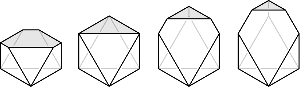
The coloring is built in a quite unintuitive way. First, we need to recall that for a polytope with the polar dual is defined as
We generalize this notion: for a vector let
| (4.1) |
Then and is obtained from by shifting facets along their normal vectors (see Figure˜4).
In the following, denotes the relative volume (relative to the affine hull of ) of a compact convex set .
Theorem 4.1 (Izmestiev [4], Theorem 2.4).
For a polytope with consider the matrix (which we shall call the Izmestiev matrix of ) with components
(in particular, is two times continuously differentiable in ). then has the following properties:
-
()
whenever .
-
()
whenever and .
-
()
has a unique negative eigenvalue of multiplicity one.
-
()
, where is the matrix introduced in \tagform@3.2.
-
()
.
Remark 4.2.
In the words of [4], the matrix constructed in Theorem˜4.1 is a Colin de Verdière matrix of the edge-graph, that is, a matrix satisfying a certain list of properties, including (i), (ii) and (iii) and the so-called strong Arnold property (for details, see e.g. [6]).
Among the Colin de Verdière matrices, one usually cares about the ones with the largest possible kernel. The dimension of this largest kernel is known as the Colin de Verdière graph invariant [6], and Theorem˜4.1 (v) then shows that . This is not too surprising and was known before. However, the result of Izmestiev is remarkable for a different reason: it shows that there is a Colin de Verdière matrix whose kernel has dimension exactly (property (v)) and that is compatible with the geometry of (property (iv)).
Remark 4.3.
Izmestiev also shows that the matrix can be expressed in terms of simple geometric properties of the polytope: for let be the dual face to the edge . Then
| (4.2) |
Definition 4.4.
The Izmestiev coloring of is defined by
where is the Izmestiev matrix of .
Observation 4.5.
Since whenever and (by Theorem˜4.1 (ii)), the colored adjacency matrix of is exactly the Izmestiev matrix .
In order to apply the “linear algebra criterion” from Section˜3, showing that is an isomorphism, we first need to show that is well-defined, that is, that is at least as symmetric as . This part is relatively straightforward if we use that the Izmestiev matrix is a linear invariant of . We include a proof for completeness:
Proposition 4.6.
is at least as symmetric as , that is, is well-defined.
Proof.
Fix a linear symmetry and let be the induced combinatorial symmetry of the edge-graph. We need to show that preserves the Izmestiev coloring, that is, .
This requires two ingredients. For the first, one checks that the generalized polar dual (like the usual polar dual) satisfies
which then gives us
| (4.3) |
where we used that holds for all linear transformations in a finite matrix group such as .
The second ingredient is the following:
| (4.4) | ||||
Putting everything together, we can show for all , and equivalently for edges. We show both at the same time by proving for all :
where we set . ∎
Theorem 4.7.
The Izmestiev coloring captures the linear symmetries of .
Proof.
By Proposition˜4.6, the Izmestiev coloring is at least as symmetric as , and so we can try to apply the “linear algebra criterion” (Theorem˜3.1) to show that captures linear symmetries. That is, we need to show that is an eigenspace of the colored adjacency matrix of . Recall that is exactly the Izmestiev matrix (Observation˜4.5), and so we can try to use the various properties of this matrix established in Theorem˜4.1.
First, (since the columns of and are dual bases of ), and so Theorem˜4.1 (iv) can be read as . Second, we have both (since is full-dimensional) and (by Theorem˜4.1 (v)). Comparing dimensions, we thus have .
We conclude that is an eigenspace of (namely, the eigenspace to eigenvalue ). The “linear algebra criterion” Theorem˜3.1 then asserts that captures the linear symmetries of . ∎
By Lemma˜2.5, if there is any coloring that captures linear symmetries, then the orbit coloring does so as well:
Corollary 4.8.
The orbit coloring captures the linear symmetries of .
Remark 4.9.
A coloring is said to be finer than a coloring if
Conversely, is said to be coarser than .
It is easy to see that the orbit coloring is the finest coloring that captures linear symmetries, that is, it uses the most colors (consider the argument in the first paragraph of Section˜2.2). In contrast, the Izmestiev coloring is in general neither the finest nor the coarsest coloring with this property. Actually determining the coarsest such coloring (i.e., using the fewest colors) seems like a challenging task.
5. Capturing orthogonal symmetries
For this section we consider the orthogonal symmetry group and all notations without an explicit hint to the kind of symmetry (such as or ) implicitly refer to their orthogonal versions.
Recall the metric coloring (Definition˜2.2) with
As previously mentioned, we consider a candidate for capturing orthogonal symmetries, but we are yet unable to prove this (see ˜6.6).
Nevertheless, combining the metric coloring and the Izmestiev coloring allows us to construct a coloring for which we can actually prove this.
Definition 5.1.
Given two colorings and , the product coloring is defined by
The relevant (and easy to verify) property of the product coloring is
| (5.1) |
In particular, if both and are well-defined, then so is .
Theorem 5.2.
The coloring captures the orthogonal symmetries of .
Proof.
The Izmestiev coloring is at least as symmetric as (we know this for linear symmetries by Proposition˜4.6, which include the orthogonal symmetries as a special case). Like-wise, the metric coloring is at least as symmetric as (every orthogonal symmetry preserves norms and inner products, and therefore also the metric coloring). So, since and are well-defined, so is .
It remains to show that has an inverse. For that, fix a . By \tagform@5.1 we have . By Theorem˜4.7 there is a corresponding with for all . It remains to show that .
Since is full-dimensional, a set that contains any vertex together with its neighbors spans , and so it suffices to verify for every two to prove the orthogonality of .
Also by \tagform@5.1, preserves the metric coloring . The claim then follows via
where we used that implies or . ∎
By (the orthogonal version of) Lemma˜2.5, if there is any coloring that captures orthogonal symmetries, then so does the orthogonal orbit coloring:
Corollary 5.3.
The orthogonal orbit coloring captures orthogonal symmetries.
6. Outlook, open questions and further notes
In this article we have shown that the edge-graph of a convex polytope, while generally a very weak representative of the polytope’s geometric nature, still has sufficient structure to let us encode two important types of geometric symmetries: linear and orthogonal symmetries. We achieved this by coloring the vertices and edges of the edge-graph.
The first coloring for which we established that it “captures the polytope’s linear symmetries” was the Izmestiev coloring (Theorem˜4.7), based on an ingenious construction by Ivan Izmestiev. But we also found that the orbit coloring, a conceptually very easy coloring, does the job as well (Corollary˜4.8). Analogous colorings exist for the orthogonal symmetries as well (Theorem˜5.2 and Corollary˜5.3).
In the following we briefly discuss various potential generalizations and follow up questions concerning these results. This further highlights the very special structure of convex polytopes that went into our theorems, emphasizing again that these results are non-trivial to achieve and to generalize.
We also want to mention the following neat consequence for “very symmetric” polytopes:
Corollary 6.1.
If is vertex- and edge-transitive (i.e., its linear resp. orthogonal symmetry group has a single orbit on vertices and edges), then is exactly as symmetric as its edge-graph.
This observation has previously been made in [7, Theorem 5.2]. No classification of simultaneously vertex- and edge-transitive polytopes is known so far, and so this fact might help in the study of this class.
6.1. Capturing other types of symmetries
Besides linear and orthogonal symmetries, there are at least two further common groups of symmetries associated with a polytope: the projective symmetries and the combinatorial symmetries (that is, the symmetries of the face lattice).
We can ask whether those too can be captured by a colored edge-graph:
Question 6.2.
Is there a coloring that captures projective resp. combinatorial symmetries:
There might be a general strategy derived from the following (informal) inclusion chain of the symmetry groups:
As it turns out, having solved the coloring problem further to the left in the chain can help to solve the problem further to the right – at least to some degree.
For example, note that every polytope can be linearly transformed via a transformation so that . That is, a coloring of that captures the orthogonal symmetries of (which has the same edge-graph) also captures the linear symmetries of . In still other words, we solved the problem of capturing linear symmetries by making use of our ability to capture orthogonal symmetries.
In our approach, we have not made use of this because we needed to solved the linear case before the orthogonal one. However, this can be of use for capturing projective symmetries. More explicitly, the question is as follows: for every polytope , is there a projective transformation so that ?
The same approach seems doomed for capturing combinatorial symmetries: there are polytopes with combinatorial symmetries that cannot be realized geometrically ([1] discusses the case of a combinatorial symmetry that cannot be made linear; to our knowledge, realizing them as projective symmetries remains to be discussed).
6.2. Edge-only coloring
For capturing the symmetries of certain 2-dimensional polytopes it is necessary to color both vertices and edges (cf. Figure˜2). But it is unclear whether this is still necessary in higher dimensions.
Question 6.3.
Is it sufficient to color only the edges if ? That is, is there an edge-only coloring that captures (for example) linear symmetries?
A vertex-only coloring is not always sufficient. For example, in even dimensions exist vertex-transitive neighborly polytopes other than the simplex: e.g. for we have the following cyclic 4-polytope with vertices that is not a simplex:
The edge-graph of is the complete graph , and has a single orbit of vertices. Thus, if is a vertex-only coloring that captures the symmetries of , then all vertices of must receive the same color. But if the edges receive no color, then . However, it is known that the linear symmetry group of the cyclic polytope other than a simplex is strictly smaller than [5].
6.3. Non-convex polytopes and general graph embeddings
Our approach suggests no immediate generalization to non-convex polytopes or various forms of polytopal complexes.
Question 6.4.
What is the most general geometric setting in which the symmetries can be “captured” by coloring the edge-graph? Does it work for non-convex and/or self-intersecting polytopes? What about more general polytopal complexes?
A vast generalization of polytope skeleta are graph embeddings. For a graph , a graph embedding is simply a map . There are natural notions of symmetry for such embeddings, and so one might ask whether it is possible to “capture” them by coloring the graph. The following example shows that this is not possible in general:
Example 6.5.
Consider the complete bipartite graph with vertex set and an embedding into defined as follows:
One can check that the linear symmetry group of this embedding acts transitively on the vertices as well as the edges. Thus, a coloring that is at least as symmetric as the graph embedding must assign the same color to all vertices, and like-wise, the same color to all edges. That is, .
However, one can also see that the given embedding has a strictly smaller symmetry group than . For example, cannot be realized as a geometric symmetry.
It might be interesting to determine conditions under which “capturing symmetries” is possible even in this very general case.
6.4. The metric coloring
It is yet unknown whether the metric coloring alone can capture orthogonal symmetries (cf. Section˜2.1 and Section˜5).
Question 6.6.
Can the metric coloring capture orthogonal symmetries?
Any potential affirmative answer to ˜6.6 will need to make use of similar assumptions as the construction of the Izmestiev coloring, namely, convexity and , as there are known counterexamples for the other cases (see Figure˜5 and Figure˜6).
An interesting special case is the following:
Question 6.7.
If is inscribed (i.e., it has all its vertices on a common sphere around the origin) and has all edges of the same length, then is it true that is as symmetric as its edge-graph, that is, ?
Acknowledgments. The author thanks Frank Göring (TU Chemnitz) for insightful discussions.
References
- [1] J. Bokowski, G. Ewald, and P. Kleinschmidt. On combinatorial and affine automorphisms of polytopes. Israel Journal of Mathematics, 47(2-3):123–130, 1984.
- [2] D. Bremner, M. Dutour Sikiric, and A. Schürmann. Polyhedral representation conversion up to symmetries. In CRM proceedings, volume 48, pages 45–72, 2009.
- [3] D. Bremner, M. D. Sikirić, D. V. Pasechnik, T. Rehn, and A. Schürmann. Computing symmetry groups of polyhedra. LMS Journal of computation and mathematics, 17(1):565–581, 2014.
- [4] I. Izmestiev. The colin de verdiere number and graphs of polytopes. Israel Journal of Mathematics, 178(1):427–444, 2010.
- [5] V. Kaibel and A. Waßmer. Automorphism groups of cyclic polytopes. 2010.
- [6] H. Van Der Holst, L. Lovász, A. Schrijver, et al. The Colin de Verdière graph parameter. Graph Theory and Computational Biology (Balatonlelle, 1996), pages 29–85, 1999.
- [7] M. Winter. The edge-transitive polytopes that are not vertex-transitive, 2020.