Carleman contraction mapping for a 1D inverse scattering problem with experimental time-dependent data
Abstract
It is shown that the contraction mapping principle with the involvement of a Carleman Weight Function works for a Coefficient Inverse Problem for a 1D hyperbolic equation. Using a Carleman estimate, the global convergence of the corresponding numerical method is established. Numerical studies for both computationally simulated and experimentally collected data are presented. The experimental part is concerned with the problem of computing dielectric constants of explosive-like targets in the standoff mode using severely underdetermined data.
Key words: one-dimensional wave equation, Carleman estimate, iterative method, contraction principle, numerical solution, experimental data, global convergence.
AMS subject classification: 35R25, 35R30
1 Introduction
We consider in this paper a 1D Coefficient Inverse Problem (CIP) for a hyperbolic PDE and construct a globally convergent numerical method for it. Unlike all previous works of this group on the convexification method for CIPs, which are cited below in this section, we construct in this paper a sequence of linearized boundary value problems with overdetermined boundary data. Each of these problems is solved using a weighted version of the Quasi-Reversibility Method (QRM). The weight is the Carleman Weight Function (CWF), i.e. this is the function, which is involved as the weight in the Carleman estimate for the corresponding PDE operator, see, e.g. [7, 4, 5, 22, 18, 31, 38, 53] for Carleman estimates. Thus, we call this method “Carleman Quasi-Reversibility Method” (CQRM). The key convergence estimate for this sequence is similar with the one of the conventional contraction mapping principle, see the first item of Remarks 8.1 in section 8. This explains the title of our paper. That estimate implies the global convergence of that sequence to the true solution of our CIP. Furthermore, that estimate implies a rapid convergence. As a result, computations are done here in real time, also, see Remark 11.1 in section 11 as well as section 12. The real time computation is obviously important for our target application, which is described below. The numerical method of this paper can be considered as the second generation of the convexification method for CIPs.
The convexification method ends up with the minimization of a weighted globally strictly convex Tikhonov functional, in which the weight is the CWF. The convexification has been developed by our research group since the first two publications in 1995 [20] and 1997 [21]. Only the theory was presented in those two originating papers. The start for numerical studies of the convexification was given in the paper [1]. Thus, in follow up publications [24, 25, 30, 16, 14, 15, 24, 25, 27, 28, 29, 32, 33, 30, 40, 50, 51] the theoritical results for the convexification are combined with the numerical ones. In particular, some of these papers work with experimentally collected backscattering data [14, 15, 26, 32, 33]. We also refer to the recently published book of Klibanov and Li [31], in which many of these results are described.
The CIP of our paper has a direct application in the problem of the standoff detection and identification of antipersonnel land mines and improvised explosive devices (IEDs). Thus, in the numerical part of this publication, we present results of the numerical performance of our method for both computationally simulated and experimentally collected data for targets mimicking antipersonnel land mines and IEDs. The experimental data were collected in the field, which is more challenging than the case of the data collected in a laboratory [14, 15, 26, 33]. The data used in this paper were collected by the forward looking radar of the US Army Research Laboratory [46]. Since these data were described in the previous publications of our research group [13, 23, 24, 25, 30, 35, 36, 51], then we do not describe them here. Those previous publications were treating these experimental data by several different numerical methods for 1D CIPs. We also note that the CIP of our paper was applied in [32, 33] to the nonlinear synthetic aperture (SAR) imaging, including the cases of experimentally collected data.
Our goal is to compute approximate values of dielectric constants of targets. We point out that our experimental data are severely underdetermined. Indeed, any target is a 3D object. On the other hand, we have only one experimentally measured time resolved curve for each target. Therefore, we can compute only a sort of an average value of the dielectric constant of each target. This explains the reason of our mathematical modeling here by a 1D hyperbolic PDE rather than by its 3D analog. This mathematical model, along with its frequency domain analog, was considered in all above cited previous publications of our research group, which were working with the experimental data of this paper by a variety of globally convergent inversion techniques.
An estimate of the dielectric constant of a target cannot differentiate with a good certainty between an explosive and a non explosive. However, we hope that these estimates, combined with current targets classification procedures, might potentially result in a decrease of the false alarm rate for those targets. We believe therefore that our results for experimental data might help to address an important application to the standoff detection and identification of antipersonnel land mines and IEDs.
Given a numerical method for a CIP, we call this method globally convergent if:
-
1.
There is a theorem claiming that this method delivers at least one point in a sufficiently small neighborhood of the true solution of that CIP without relying on a good initial guess about this solution.
-
2.
This theorem is confirmed numerically.
CIPs are both highly nonlinear and ill-posed. As a result, conventional least squares cost functionals for them are non convex and typically have many local minima and ravines, see, e.g. [49] for a numerical example of this phenomenon. Conventional numerical methods for CIPs are based on minimizations of those functionals, see, e.g. [8, 11, 12]. The goal of the convexification is to avoid local minima and ravines and to provide accurate and reliable solutions of CIPs.
In the convexification, a CWF is a part of a certain least squares cost functional , where is the parameter of the CWF. The presence of the CWF ensures that, with a proper choice of the parameter the functional is strictly convex on a certain bounded convex set of an arbitrary diameter in a Hilbert space. It was proven later in [1] that the existence and uniqueness of the minimizer of on are also guaranteed. Furthermore, the gradient projection method of the minimization of on converges globally to that minimizer if starting at an arbitrary point of . In addition, if the level of noise in the data tends to zero, then the gradient projection method delivers a sequence, which converges to the true solution. Thus, since is an arbitrary number, then this is the global convergence, as long as numerical studies confirm this theory. Furthermore, it was recently established in [33, 40] that the gradient descent method of the minimization of on also converges globally to the true solution.
First, we come up with the same boundary value problem (BVP) for a nonlinear and nonlocal hyperbolic PDE as we did in the convexification method for the same 1D CIP in [30]. The solution of this BVP immediately provides the target unknown coefficient. However, when solving this BVP, rather than constructing a globally strictly convex cost functional for this BVP, as it was done in [30] and other works on the convexification, we construct a sequence of linearized BVPs. Just as the original BVP, each BVP of this sequence involves a hyperbolic operator with non local terms and overdetermined boundary conditions.
Because of non local terms and the overdetermined boundary conditions, we solve each BVP of this sequence by the new version of the QRM, the Carleman Quasi-Reversibility Method (CQRM). Indeed, the classical QRM solves ill-posed/overdetermined BVPs for linear PDEs, see [37] for the originating work as well as, e.g. [19, 31] for updates. Convergence of the QRM-solution to the true solution is proven via an appropriate Carleman estimates [19, 31]. However, a CWF is not used in the optimizing quadratic functional of the conventional QRM of [19, 31]. Unlike this, a CWF is involved in CQRM. It is exactly the presence of the CWF, which enables us to derive the above mentioned convergence estimate, which is an analog of the one of the contraction principle. This allows us, in turn to establish convergence rate of the sequence of CQRM-solutions to the true solution of that BVP. The latter result ensures that our method is a globally convergent one.
Various versions of the second generation of the convexification method involving CQRM were previously published in [2, 3, 45, 44, 39]. In these publications, globally convergent numerical methods for some nonlinear inverse problems are presented. In [2, 3] CIPs for hyperbolic PDEs in are considered. The main difference between [2, 3] and our work is that it is assumed in [2, 3] that one of initial conditions is not vanishing everywhere in the closed domain of interest. In other words, papers [2, 3] work exactly in the framework of the Bukhgeim-Klibanov method, see [6] for the originating work on this method and, e.g. [4, 5, 17, 22, 18, 31, 53] for some follow up publications. On the other hand, in all above cited works on the convexification, including this one, either the initial condition is the function, or a similar requirement holds for the Helmholtz equation. The only exception is the paper [29], which also works within the framework of the method of [6]. We refer to papers [10, 34] for some numerical methods for CIPs with the Dirichlet-to-Neumann map data. In these works the number of free variables in the data exceeds the number of free variables in the unknown coefficient, In our paper Also, in all other above cited works on the convexification.
There is a classical Gelfand-Levitan method [41] for solutions of 1D CIPs for some hyperbolic PDEs. This method does not rely on the optimization, and, therefore, avoids the phenomenon of local minima. It reduces the original CIP to a linear integral equation of the second kind. This equation is called “Gelfand-Levitan equation” (GL). However, the questions about uniqueness and stability of the solution of GL for the case of noisy data is open, see, e.g. Lemma 2.4 in the book [48, Chapter 2]. This lemma is valid only in the case of noiseless data. However, the realistic data are always noisy. In addition, it was demonstrated numerically in [13] that GL cannot work well for exactly the same experimental data as the ones we use in the current paper. On the other hand, it was shown in [24, 25, 51] that the convexification works well with these data. The same is true for the method of the current paper.
Uniqueness and Lipschitz stability theorems of the CIP considered here are well known. Indeed, it was shown in, e.g. [51] that, using the same change of variables as the one considered in section 2 below, one can reduce our CIP to a similar CIP for the equation with the unknown coefficient We refer to [48, Theorem 2.6 of Chapter 2] for the Lipschitz stability estimate for the latter CIP. In addition, both uniqueness and Lipschitz stability results for our CIP actually follow from Theorem 8.1 below as well as from the convergence analysis in two other works of our research group on the convexification method for this CIP [30, 51].
This paper is arranged as follows. In section 2 we state both forward and inverse problems. In section 3 we derive a nonlinear BVP with non local terms. In section 4 we describe iterations of our method to solve that BVP. In section 5 we formulate the Carleman estimate for the principal part of the PDE operator of that BVP. In section 6 we prove the strong convexity of a functional of section 5 on an appropriate bounded set. In section 7 we formulate two methods for finding the unique minimizer of that functional: gradient descent method and gradient projection method and prove the global convergence to the minimizer for each of them. In section 8 we establish the contraction mapping property and prove the global convergence of the method of section 4. In section 9 we formulate two more global convergence theorems, which follow from results of sections 7 and 8. Numerical results with simulated and experimental data are presented in Section 10 and 11 respectively. Concluding remarks are given in section 12.
2 Statements of Forward and Inverse Problems
Below all functions are real valued ones. Let be a known number, be the spatial variable and the function , represents the spatially distributed dielectric constant. We assume that
| (2.1) | ||||
| (2.2) |
where is a small number. Let be a positive number. We consider the following Cauchy problem for a 1D hyperbolic PDE with a variable coefficient in the principal part of the operator:
| (2.3) |
| (2.4) |
The problem of finding the function from conditions (2.3), (2.4) is our Forward Problem.
Let be the travel time needed for the wave to travel from the point source at to the point ,
| (2.5) |
By (2.5) the following 1D analog of the eikonal equation is valid:
| (2.6) |
Let be the Heaviside function,
Lemma 2.1 [30, Lemma 2.1]. For , the function has the form
| (2.7) |
where the function Furthermore,
| (2.8) |
Lemma 2.2 [Absorbing boundary condition] [30, 50]. Let be the number in (2.1). Let and be two arbitrary numbers. Then the solution of Forward Problem (2.3), (2.4) satisfies the absorbing boundary condition at and , i.e.
| (2.9) |
| (2.10) |
We are interested in the following inverse problem:
Coefficient Inverse Problem (CIP). Suppose that the following two functions , are known:
| (2.11) |
Determine the function for , assuming that the number in (2.1) is known.
3 A Boundary Value Problem for a Nonlinear PDE With Non-Local Terms
We now introduce a change of variable
| (3.1) |
We will consider the function only for Using (2.6) and (3.1), we obtain
| (3.2) |
Furthermore, it follows from (2.8)
| (3.3) |
Substituting (2.6), (3.3) and (3.4) in (3.2), we obtain
| (3.5) |
Equation, (3.5) is a nonlinear PDE with respect to the function with nonlocal terms and . We now need to obtain boundary conditions for the function By (2.2) and (2.5) for Hence, (2.11), (2.12) and (3.1) lead to
| (3.6) |
We will solve equation (3.5) in the rectangle
| (3.7) |
By (3.1)
| (3.8) |
By (2.1), (2.2) and (2.5) . Hence, using (2.9) and (3.8), we obtain
| (3.9) |
It follows from (2.1) and (3.3) that
| (3.10) |
In addition, we need and we also need to bound the norm from the above. Let be an arbitrary number. We define the set as
| (3.11) |
We assume below that
| (3.12) |
By embedding theorem and
| (3.13) |
where the constant depends only on the domain Using (3.10), we define the function as:
| (3.17) | |||||
Then the function is piecewise continuously differentiable in and by (3.13) and (3.17)
| (3.18) |
| (3.19) |
Thus, (3.5), (3.6), (3.9), (3.17) and (3.19) result in the following BVP for a nonlinear PDE with non-local terms:
| (3.20) |
| (3.21) |
Thus, we focus below on the numerical solution of the following problem:
4 Numerical Method for Problem 3.1
4.1 The function
We now find the first approximation for the function Using (2.2), we choose as the first guess for the function Hence, by (3.3),
| (4.1) |
We now need to find the function To do this, drop the nonlinear third term in the left hand side of equation (3.20) and, using (4.1) and (3.17), set . Then (3.20), (3.21) become:
| (4.2) |
| (4.3) |
BVP (4.2), (4.3) has overdetermined boundary conditions (4.3). Typically, QRM works well for BVPs for PDEs with overdetermined boundary conditions [19, 31]. Therefore, we solve BVP (4.2), (4.3) via CQRM. This means that we consider the following minimization problem:
Minimization Problem Number . Assuming (3.12), minimize the functional on the set ,
| (4.4) |
where is the Carleman Weight Function for the operator [50, 51]
| (4.5) |
where is the parameter, and is the regularization parameter. Both parameters will be chosen later.
Theorem 6.1 guarantees that, for appropriate values of parameters there exists unique minimizer of the functional
4.2 The function for
5 The Carleman Estimate
In this section we formulate the Carleman estimate, which is the main tool of our construction. This estimate follows from Theorem 3.1 of [30] as well as from (3.18). Let be an arbitrary function and let the function be constructed from the function as in (3.17). Consider the operator
Theorem 5.1 (Carleman estimate [30]). There exists a number depending only on such that for any there exists a sufficiently large number depending only on , such that for all and for all functions the following Carleman estimate holds:
| (5.1) |
Remark 5.1. Here and everywhere below denotes different constants depending only on listed parameters.
6 Strict Convexity of Functional (4.8) on the Set , Existence and Uniqueness of Its Minimizer
Functional (4.8) is quadratic. We prove in this section that it is strictly convex on the set In addition, we prove existence and uniqueness of its minimizer on this set. Although similar results were proven in many of the above cited publications on the convexification, see, e.g. [30] for the closest one, there are some peculiarities here, which are important for our convergence analysis, see Remarks 6.1, 6.2 below.
Introduce the subspace as:
| (6.1) |
Denote the scalar product in the space Also, denote
| (6.2) |
| (6.3) |
Theorem 6.1. 1. For any set of parameters and for any the functional has the Fréchet derivative The formula for is:
| (6.4) |
for all
2. This derivative is Lipschitz continuous in , i.e. there exists a constant such that
| (6.5) |
3. Let and be the numbers of Theorem 5.1. Then there exists a sufficiently large constant
| (6.6) |
depending only on listed parameters such that for all and for all the functional is strictly convex on the set More precisely, let be an arbitrary function and also let the function Then the following inequality holds:
| (6.7) |
4. For any there exists unique minimizer
| (6.8) |
of the functional on the set and the following inequality holds:
| (6.9) |
where denotes the scalar product in
Remark 6.1. Even though the expression in the right hand side of (6.4) is linear with respect to the function we cannot use Riesz theorem here to prove existence and uniqueness of the minimizer at which Rather, all what we can prove is (6.9). This is because we need to ensure that the function .
Proof of Theorem 6.1. Since both function satisfy the same boundary conditions, then
| (6.10) |
| (6.11) |
The expression in the first line of (6.11) coincides with expression in the right hand side of (6.4). In fact, this is a bounded linear functional mapping in . Therefore, by Riesz theorem, there exists unique function such that
In addition, it is clear from (6.11) and (LABEL:5.9) that
Therefore,
| (6.12) |
is the Fréchet derivative of the functional at the point and the right hand side of (6.4) indeed represents Estimate (6.5) obviously follows from (6.4).
We now prove strict convexity estimate (6.7). To do this, we apply Carleman estimate (5.1) to the third line of (6.11). We obtain
| (6.13) |
By trace theorem there exists a constant depending only on the domain such that
Since the regularization parameter then we can choose so large that
Hence, for these values of the expression in the last line of (6.13) can be estimated from the below as:
| (6.14) |
Hence, (6.13) and (6.14) imply
This proves (6.7). The existence and uniqueness of the minimizer and inequality (6.9) follow from (6.7) as well as from a combination of Lemma 2.1 and Theorem 2.1 of [1], also see [42, Chapter 10, section 3].
Remark 6.2. Since the functional is quadratic, then its strict convexity on the whole space follows immediately from the presence of the regularization term in it. However, in addition to the claim of its strict convexity, we actually need in our convergence analysis below those terms in the right hand side of the strict convexity estimate (6.7), which are different from the term These terms are provided by Carleman estimate (6.7). The condition of Theorem 6.1 is imposed to dominate the negative term in the last line of (6.7).
7 How to Find the Minimizer
Since we search for the minimizer of functional (4.8) on the bounded set rather than on the whole space then we cannot just use Riesz theorem to find this minimizer, also see [1] and [42, Chapter 10, section 3] for the case of finding a minimizer of a strictly convex functional on a bounded set. Two ways of finding the minimizer are described in this section.
7.1 Gradient descent method
Keeping in mind (3.12), choose an arbitrary function We arrange the gradient descent method of the minimization of functional (4.8) as follows:
| (7.1) |
where is a small number, which is chosen later. It is important to note that since functions then boundary conditions (4.7) are kept the same for all functions Also, using (3.17) and (4.9), we set
| (7.2) |
| (7.3) |
Theorem 7.1 claims the global convergence of the gradient descent method (7.1) in the case when
Theorem 7.1. Let the number be the one defined in (6.6). Let . For this value of let be the unique minimizer of the functional on the set with the regularization parameter (Theorem 6.1). Assume that the function For each choose the starting point of the gradient descent method (7.1) as Then, there exists a number such that for any all functions Furthermore, there exists a number such that the following convergence estimates are valid:
| (7.4) |
| (7.5) |
7.2 Gradient projection method
Suppose now that there is no information on whether or not the function In this case we construct the gradient projection method. We introduce the function since it is easy to construct the projection operator on a ball with the center at
Suppose that there exists a function such that
| (7.6) |
This function exists, for example, in the case when the function Indeed, as one of examples of this function (among many), one can take, e.g.
where the function is such that
The existence of such functions is well known from the Analysis course. Denote
| (7.7) |
| (7.8) |
| (7.9) |
Assume that
| (7.10) |
By (7.7), (7.9), (7.10) and triangle inequality
| (7.11) |
To find the function satisfying conditions (7.8), (7.9), we minimize the following functional
| (7.12) |
Remark 7.1. An obvious analog of Theorem 6.1 is valid of course for functional (7.12). But in this case we should have instead of (6.6) In particular, there exists unique minimizer of this functional on the closed ball We omit the formulation of this theorem, since it is an obvious reformulation of Theorem 6.1.
Let be the projection operator of the space on the closed ball Then this operator can be easily constructed:
We now construct the gradient projection method of the minimization of the functional on the set Let be an arbitrary function. Then the sequence of the gradient projection method is:
| (7.13) |
where is a small number, which is chosen later. Using (7.2), (7.3) and (7.7), we set
| (7.14) |
| (7.15) |
Here the function is obtained as follows: First, we consider the function Next, we apply procedure (3.17) to this function. Similarly for
Denote the unique minimizer of functional (7.12) on the set (Remark 7.1). Following (7.7), denote
| (7.16) |
We omit the proof of Theorem 7.2 since it is very similar with the proof of Theorem 7.1. The only difference is that instead of Theorem 4.6 of [33] one should use Theorem 4.1 of [30].
Theorem 7.2. Let (7.6), (7.10) hold. Let the number be the one defined in (6.6) and let
For this value of and for let be the unique minimizer of functional (7.12) on the set (Remark 7.1). Let notations (7.14) hold. For each choose the starting point of the gradient projection method (7.1) as Then there exists a number such that for any there exists a number such that the following convergence estimates are valid for the iterative process (7.13):
Remark 7.2. Both theorems 7.1 and 7.2 claim the global convergence of corresponding minimization procedures. This is because the starting function in both cases is an arbitrary one either in or in and a smallness condition is not imposed on the number .
8 Contraction Mapping and Global Convergence
In this section, we prove the global convergence of the numerical method of section 4 for solving Problem 3.1. To do this, we introduce first the exact solution of our CIP. Recall that the concept of the existence of the exact solution is one of the main concepts of the theory of ill-posed problems [4, 52]. In particular, an estimate in our global convergence theorem is very similar to the one in contraction mapping.
Suppose that there exists a function satisfying conditions (2.1), (2.2). Let be the solution of problem (2.3), (2.4) with We assume that the corresponding data for the CIP are noiseless, see (2.11), (2.12). Let be the function which is constructed from the function as in (3.1). Following (3.11), we assume that
| (8.1) |
| (8.2) |
| (8.3) |
| (8.4) |
By (3.3)
| (8.5) |
It is important in the formulation of Theorem 6.1 that both functions and should have the same boundary conditions as prescribed in However, boundary conditions for functions and are different. Hence, similarly to subsection 7.2, we consider a function such that (see (7.6))
| (8.6) |
We assume similarly to (7.10) that
| (8.7) |
Also, similarly to (7.7), we introduce the function as:
| (8.8) |
Let be the number defined in (6.6), let and the function (see (6.8)) be the unique minimizer of the functional on the set the existence of which is established in Theorem 6.1. Following (7.7), denote
| (8.9) |
By (6.8), (7.11), (8.1), (8.2) and (8.7)-(8.9)
| (8.10) |
Also, it follows from embedding theorem, (3.13), (6.8), (7.10), (8.7) and (8.10) that
| (8.11) |
We assume that the data for our CIP are given with noise of the level where the number is sufficiently small. More precisely, we assume that
| (8.12) |
Observe that (3.17), (8.1) and (8.2) imply that
| (8.13) |
By (8.3), (8.4), (8.6) and (8.8)
| (8.14) |
in and
| (8.15) |
Theorem 8.1 (contraction mapping and global convergence of the method of section 3). Let functions , satisfy conditions (7.6), (7.10), (8.6), (8.7) and (8.12). Let a sufficiently large number be the one defined in (6.6). Let
| (8.16) |
For this value of let be the unique minimizer of the functional on the set with the regularization parameter (Theorem 6.1). Let
| (8.17) |
where is defined in (7.3). Then the following convergence estimate holds
| (8.18) |
which leads to:
| (8.19) |
In addition,
| (8.20) |
Remarks 8.1:
1. Due to the presence of the term with a sufficiently large , estimate (8.18) is similar to the one in the classic contraction mapping principle, although we do not claim here the existence of the fixed point. This explains the title of our paper.
2. When computing the unique minimizer of functional (4.4) on the set we do not impose a smallness condition on the number . Therefore, Theorem 8.1 claims the global convergence of the method of section 4, see Introduction for our definition of the global convergence. The same is true for Theorems 9.1 and 9.2 in the next section.
Consider the functional Since both functions and have the same zero boundary conditions (7.9) and since by (8.10) both of them belong to the set , then the analog of Theorem 6.1, which is mentioned in Remark 7.1, implies (see (6.7))
| (8.23) |
By (6.9)
Hence, the left hand side of (8.23) can be estimated as:
| (8.24) |
We now estimate the right hand side of (8.24) from the above. It follows from (4.8), (7.12) and (8.3) that
| (8.25) |
where
| (8.26) |
By (8.3), the third line of (8.26) equals zero. Hence, (8.26) becomes
Hence, by (3.17), (8.12) and embedding theorem
| (8.27) |
Using (8.12) and (8.13), we obtain
Combining this with (8.27), we obtain
| (8.28) |
Next,
where the function can be estimated as
| (8.29) |
Hence,
Hence, using (3.11), (3.17), (8.1), (8.13) and (8.29), we obtain
| (8.30) |
Combining (8.28) with (8.30), we obtain
Hence, by (8.25)
Substituting this in (8.24) and then using (8.23), we obtain
| (8.31) |
Obviously
| (8.32) |
| (8.33) |
Denote
| (8.34) |
| (8.35) |
Iterating (8.35) with respect to we obtain
| (8.36) |
Apply (8.21) to the left hand side of estimate (8.36). Also, apply (8.22) at to the right hand side of (8.36). We obtain (8.19). Estimate (8.20) follows from an obvious combination of (8.19) with (7.3), (8.5), (8.13) and (LABEL:8.150). Finally, estimate (8.18) follows immediately from (8.21), (8.22) and (8.31).
9 Global Convergence of the Gradient and Gradient Projection Methods to the Exact Solution
First, we consider the gradient method of the minimization of functionals on the set see (7.1). The proof of Theorem 9.1 follows immediately from the triangle inequality combined with Theorems 7.1 and 8.1.
Theorem 9.1. Let and be the numbers of Theorem 5.1. Let the sufficiently large number be the one defined in (6.6). Let the number be the same as in (8.16),
Let and let the regularization parameter Assume that the functions for all For each , choose the starting point of the gradient method (7.1) as Then there exists a number such that for any all functions Furthermore, there exists a number such that the following convergence estimate is valid:
where the function is defined in (8.17).
Consider now the gradient projection method of the minimization of the functionals in (7.12) on the set , see (7.13). We use notations (7.14). Theorem 9.2 follows immediately from the triangle inequality combined with Theorems 7.2 and 8.1.
Theorem 9.2. Let the number be the one defined in (6.6). Let the number be the same as in (8.16),
Let and let the regularization parameter Consider the gradient projection method (7.13). For each , choose the starting point of this method as an arbitrary point of the ball Then there exists a number such that for any there exists a number such that the following convergence estimate is valid:
where functions and are defined in (7.14), (7.16) and (8.17) respectively.
10 Numerical Studies
10.1 Numerical implementation
To generate the simulated data, by Lemma 2.2, we solve problem (2.3), (2.4) for the case when the whole real line is replaced by a large interval with the absorbing boundary conditions (2.9)–(2.10). More precisely, just as in Section 6.1 of [30], we use the implicit scheme to numerically solve
| (10.1) |
where , and
is a smooth approximation of the Dirac function . We solve problem (10.1) by the implicit finite difference method. In the finite difference scheme, we arrange a uniform partition for the interval as with , , where is a large number. In the time domain, we split the interval into uniform sub-intervals , , with where is a large number. In our computational setting, and . These numbers are the same as in [30].
We observe a computational error for the function near . This is due to the fact that the function is not exactly equal to the Dirac function. We correct the error as follows. It follows from (2.2), (2.7) and (2.8) that in a neighborhood of the point We, therefore, replace the data by when is small. In our computation, we set for . This data correction step is exactly the same as in Section 6.1 of [30] and is illustrated by Figure 2 in that publication. Then, we can extract the noiseless data easily. We next add the noise into the data via the formula
| (10.2) |
where is the noise level and rand is the function that generates uniformly distributed random numbers in the range In all numerical tests with simulated data below, the noise level i.e. Due to (2.12), the function Due to the presence of noise, see (10.2), we cannot compute by the finite difference method. Hence, the function is computed by the Tikhonov regularization method. The version of the Tikhonov regularization method for this problem is well-known. Hence, we do not describe this step here.
Having the data for the function in hand, we proceed as in Algorithm 1.
In step 1 of Algorithm 1, we choose , and These parameters were chosen by a trial-error process that is similar to the one in [50]. Just as in [50], we choose a reference numerical test in which we know the true solution. In fact, test 1 of section 10.2 was our reference test. We tried several values of and until the numerical solution to that reference test became acceptable. Then, we have used the same values of these parameters for all other tests, including all five (5) available cases of experimental data.
We next implement Steps 2 and 3 of Algorithm 1. We write differential operators in the functionals and in the finite differences with the step size in space and the step size in time and minimize resulting functionals with respect to values of corresponding functions at grid points. Since the integrand in the definitions of the functional is the square of linear functions, then its minimizer is its critical point. In finite differences, we can write a linear system whose solution is the desired critical point. We solve this system by the command “lsqlin” of Matlab. The details in implementation by the finite difference method including the discretization, the derivation of the linear system for the critical point, and the use of “lsqlin” are very similar to the scheme in [43, 47]. Recall that in our theory, in the definition of the functional acting on , see (4.8), we replaced with its analog which belongs to the bounded set and also replaced with . These replacements are only for the theoretical purpose to avoid the case when blows up. However, in the numerical studies, these steps can be relaxed. This means that in Step 3, we have minimized the finite difference analog of the functional
| (10.3) |
subject to the boundary conditions in lines 2 and 3 of (3.11). Another numerical simplification is that rather than using the norm in the regularization term, we use the norm in (10.3). Although the theoretical analysis supporting the above simplifications is missing, we did not experience any difficulties in computing the numerical solutions to Problem 3.1. All of our numerical results are satisfactory.
10.2 Numerical results for computationally simulated data
To test Algorithm 1, we present four (4) numerical examples.
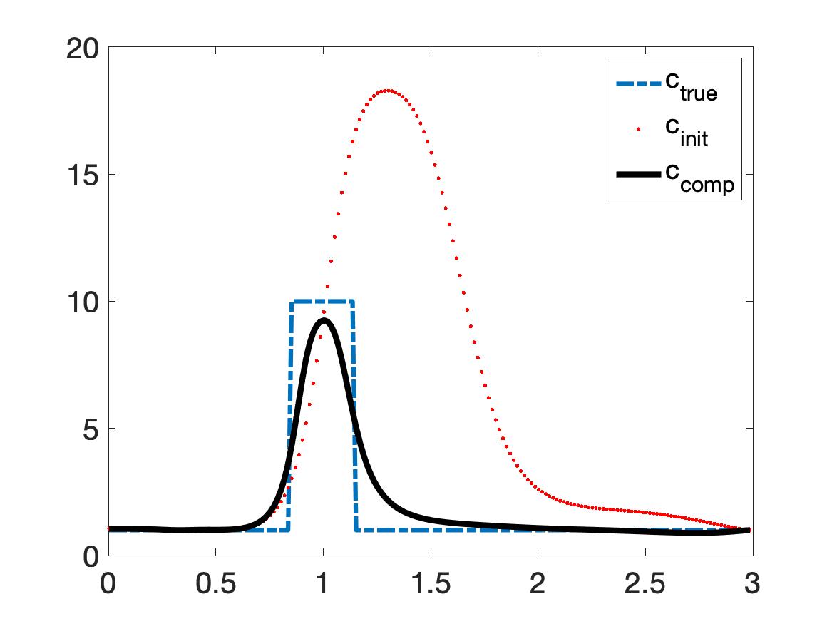
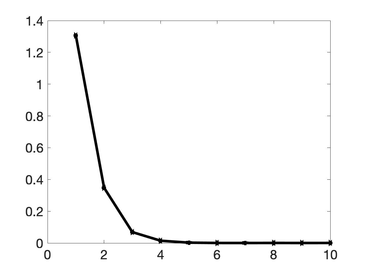
Test 1 (the reference test). We first test the case of one inclusion with a high inclusion/background contrast. The true dielectric constant function has the following form
| (10.4) |
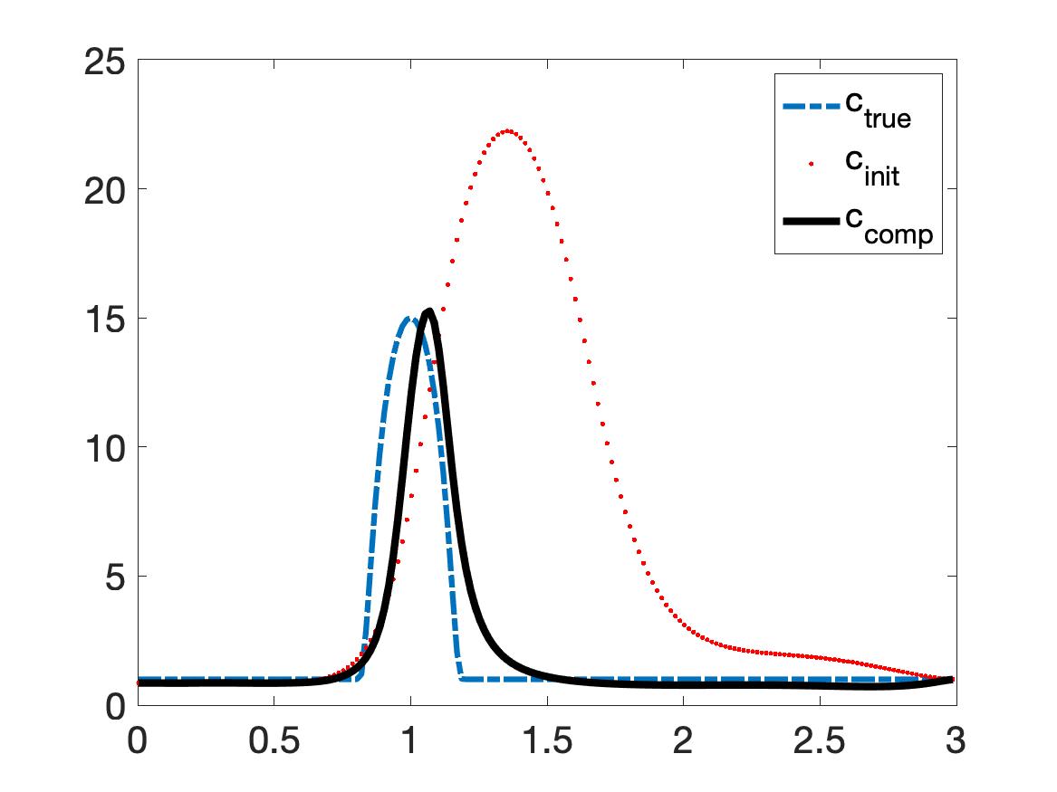
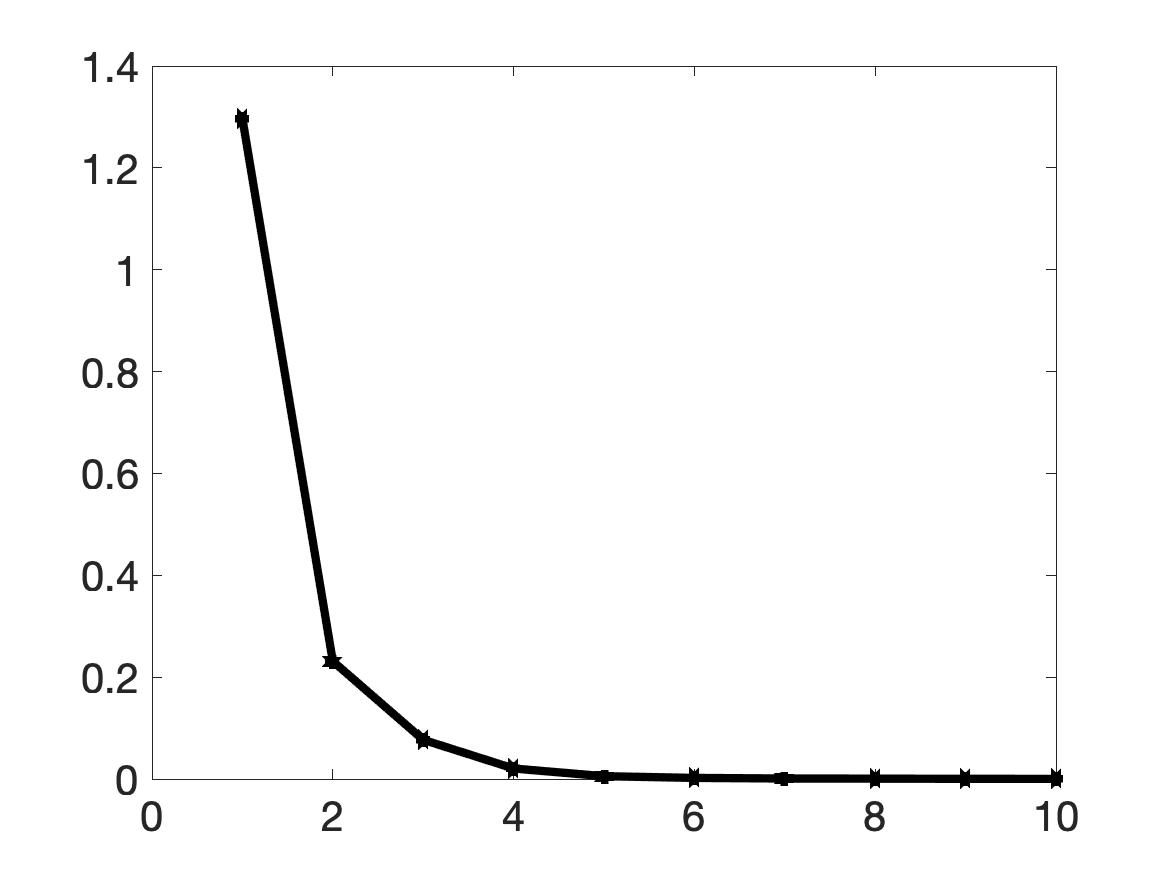
Thus, the inclusion/background contrast as 15:1. It is evident from Figure 1 that we can successfully detect an object. The diameter of this object is 0.4 and the distance between this object and the source is 1. The true inclusion/background contrast is 15/1. The maximal value of the computed dielectric constant is 15.28. The relative error in this maximal value is 1.89% while the noise level in the data is 5%. Although the contrast is high, our method provides good numerical solution without requiring any knowledge of the true solution. Our method converges fast. Although the initial reconstruction computed in Step 2 of Algorithm 1 is not very good, see Figure 1a, one can see in Figure 1b, that the convergence occurs after only five (5) iterations. This fact verifies numerically the “contraction property” of Theorem 8.1 including the key estimate (8.20).
Test 2. The true function in this test has two “inclusions”,
| (10.5) |
Numerical results of this test are displayed in Figure 2.
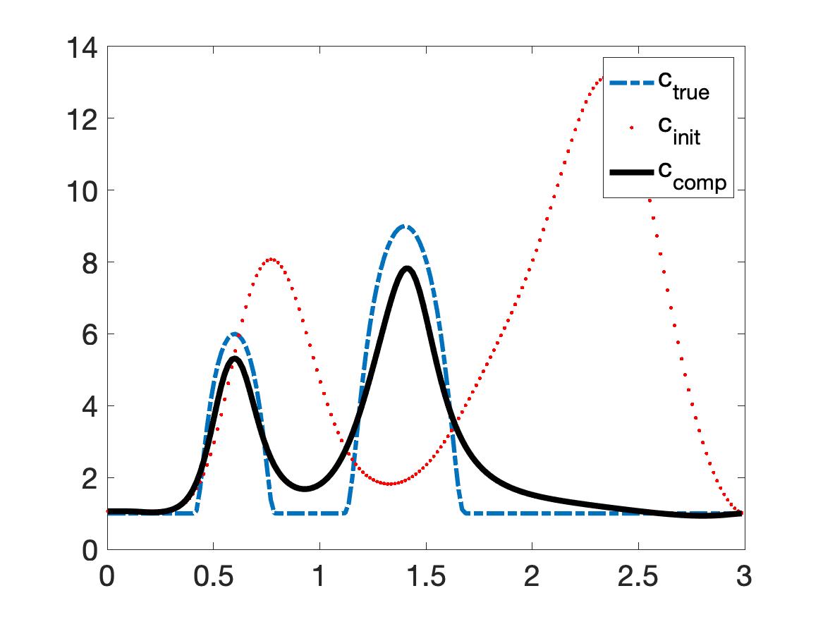
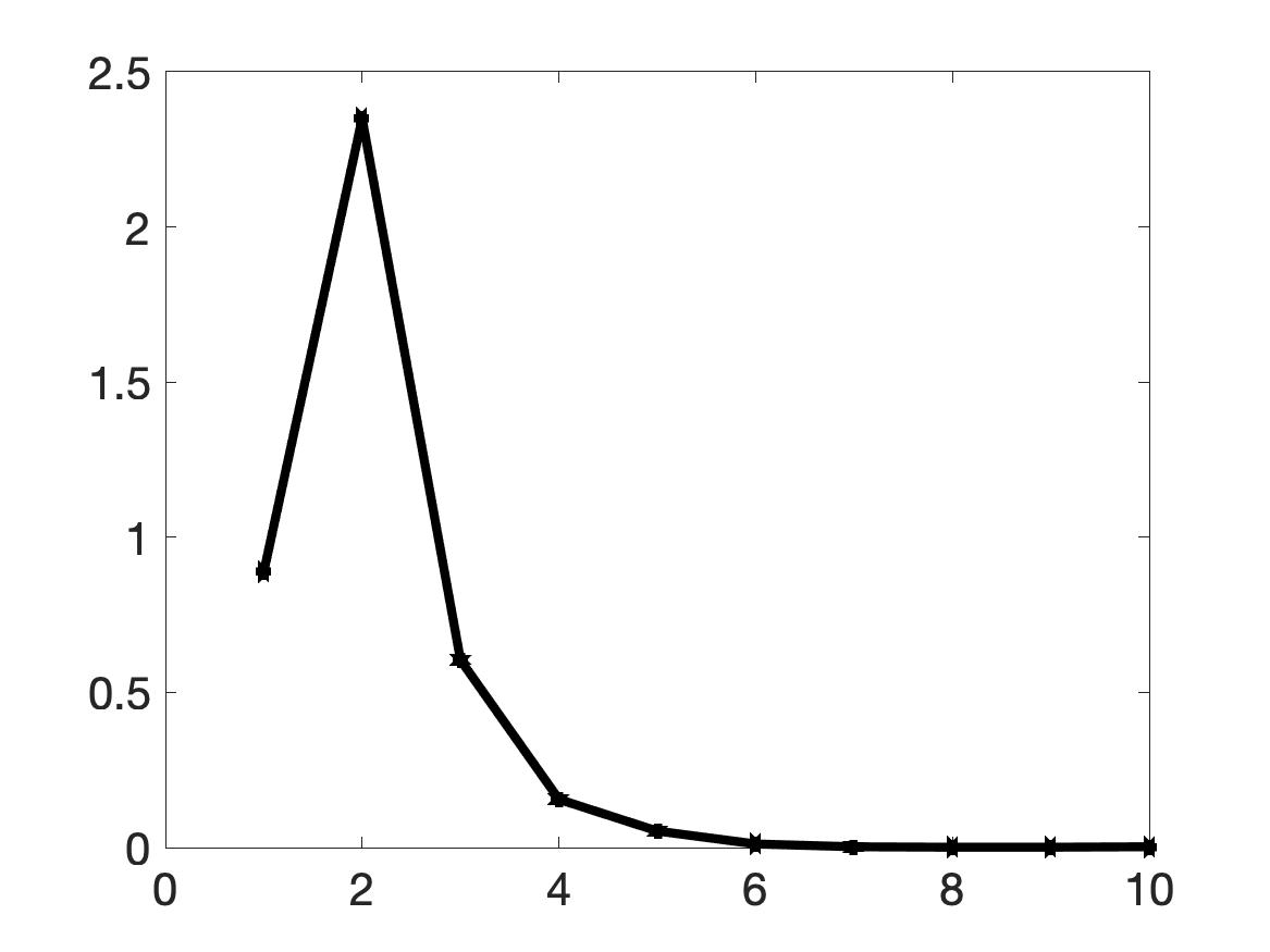
Test 2 is more complicated than Test 1. However, we still obtain good numerical results. It is evident from Figure 2a that we can precisely detect the two inclusions without any initial guess. The true maximal values of the dielectric constant of the inclusions in the left and the right are 6 and 9 respectively. The reconstructed maximal values in those inclusions are acceptable. They are 5.31 (relative error 11.5%) and 7.8 (relative error 13.3%). As in Test 1, the initial reconstruction computed in Step 2 of Algorithm 1 is far from Still, our iterative procedure converges after 7 iterations, see Figure 2b.
Test 3 We test the case when the function is discontinuous. It is a piecewise constant function given by
| (10.6) |
The numerical solution for this test is presented in Figure 3.
Although the function is not smooth and actually not even continuous, Algorithm 1 works and provides a reliable numerical solution. The computed maximal value of the dielectric constant of the object is 9.25 (relative error 7.5%), which is acceptable. The location of the object is detected precisely, see Figure 3a. As in the previous two tests, Algorithm 1 converges fast. After the fifth iteration, the reconstructed function becomes unchanged. Again, this fact numerically confirms both Theorem 8.1 and the robustness of our method.
Test 4 In this test, the function has the following form:
| (10.7) |
This test is interesting since the graph of the function (10.7) consists of a curve and an inclusion. The numerical solution for this case is presented in Figure 4.
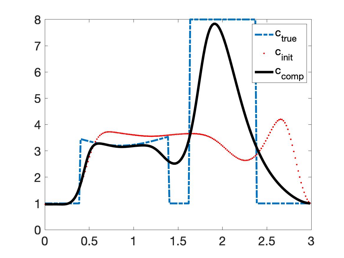
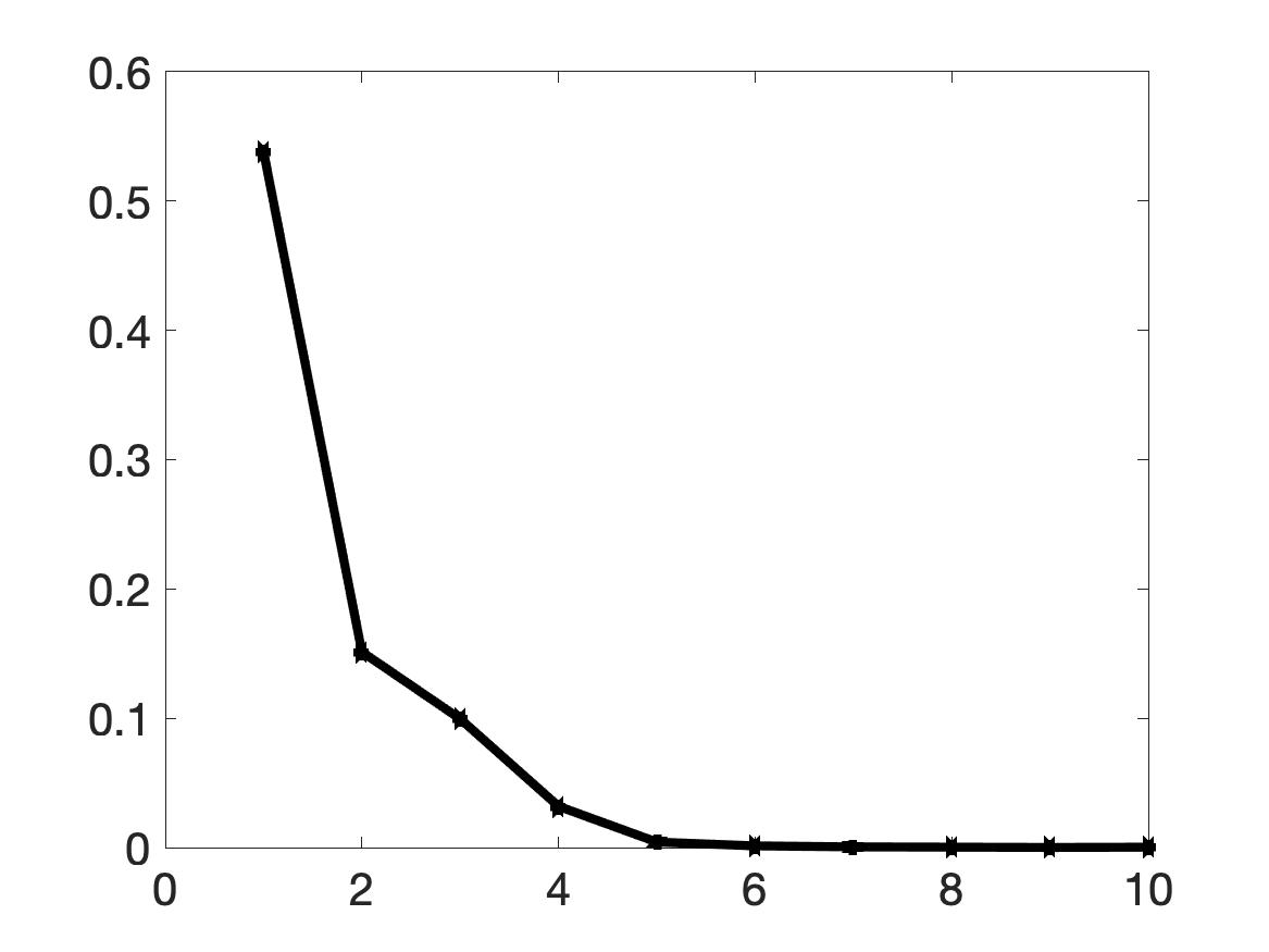
One can observe from Figure 4a that our method to compute the initial reconstruction in Step 2 of Algorithm 1 is not very effective. However, after only 6 iterations, good numerical results are obtained. The curve in the first inclusion locally coincides with the true one and the maximal value of the computed dielectric constant within inclusion is quite accurate: it is 7.83 (relative error 2.12%). Our method converges at the iteration number 6.
Remark 10.1.
It follows from all above tests that Algorithm 1 is robust in solving a highly nonlinear and severely ill-posed Problem 3.1. It provides satisfactory numerical results with a fast convergence. For each test, the computational time to compute the numerical solution is about 29 seconds on a MacBook Pro 2019 with 2.6 GHz processor and 6 Intel i7 cores. This is almost a real time computation.
11 Numerical Results for Experimental Data
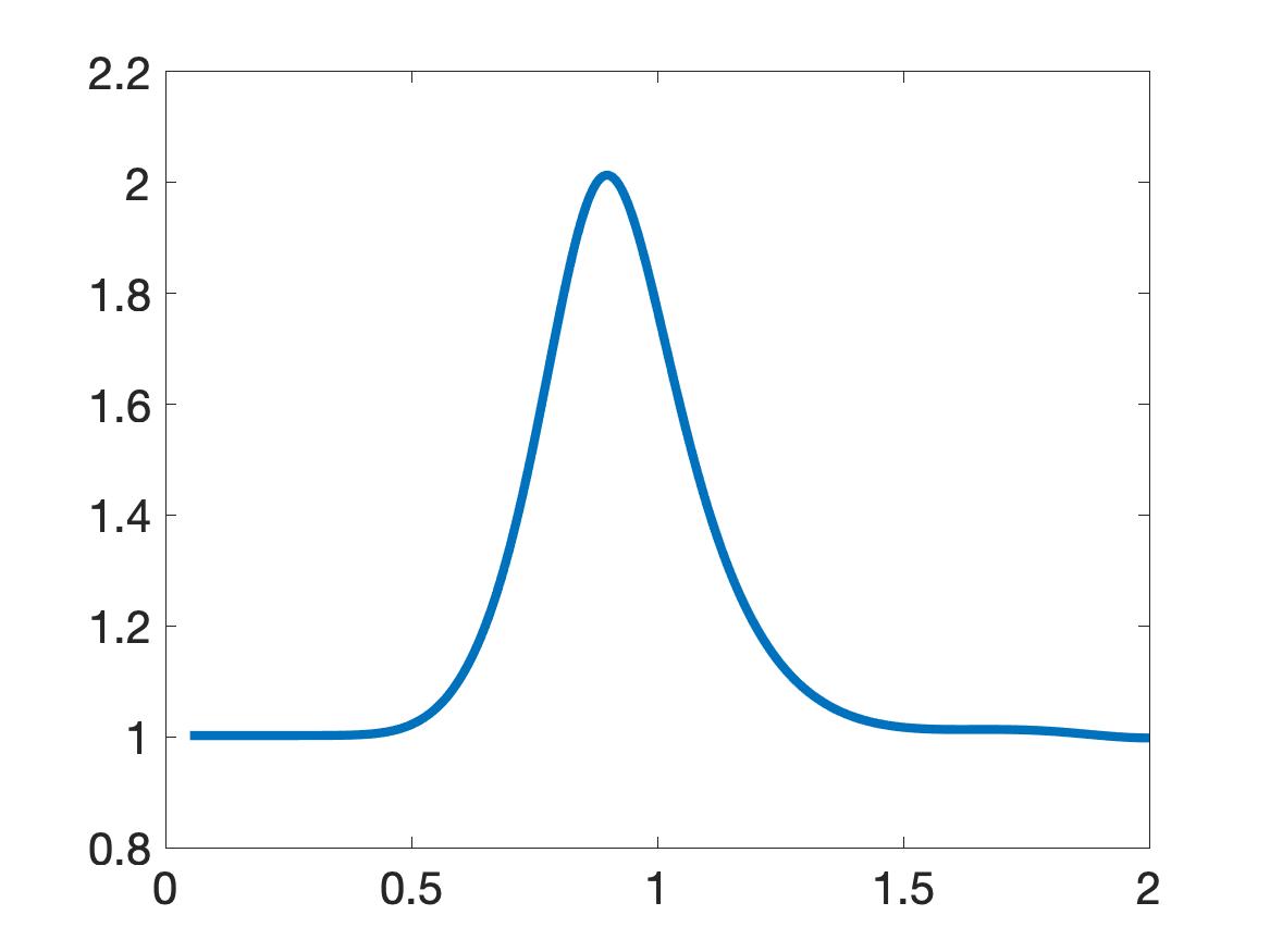
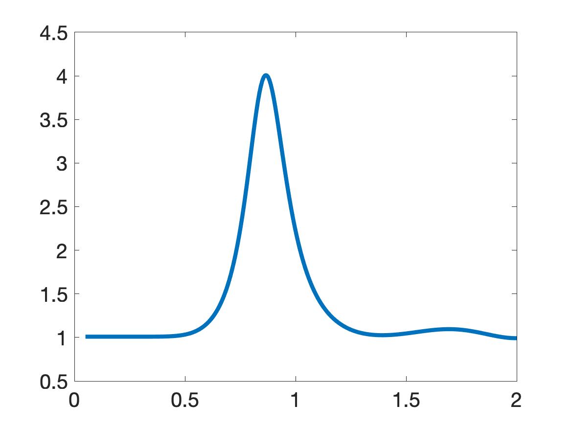
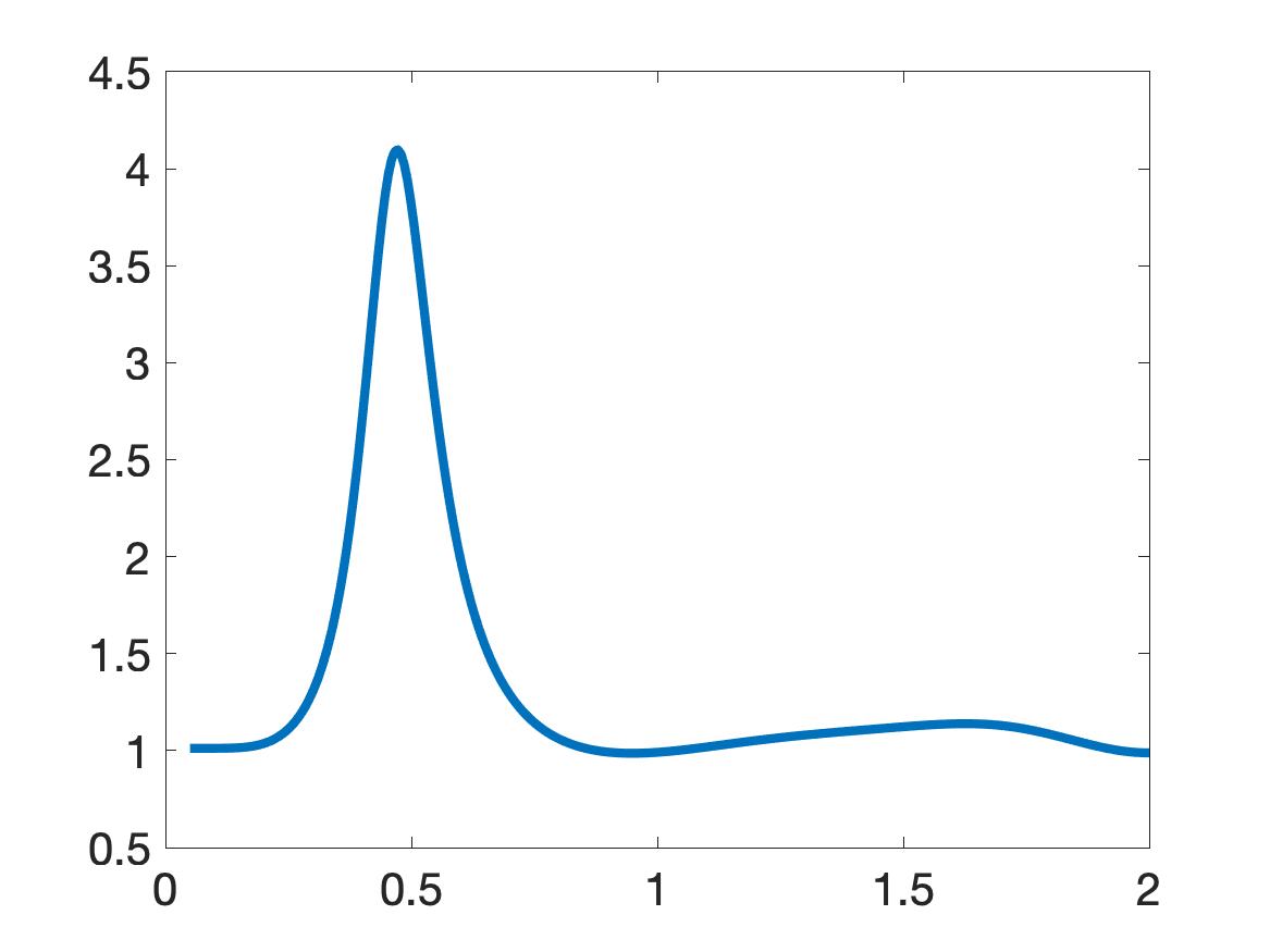
The experimental data we use to test Algorithm 1 were collected by the Forward Looking Radar built in the US Army Research Laboratory [46]. The data were initially collected to detect and identify targets mimicking shallow anti-personnel land mines and IEDs. Five mimicking devices were: a bush, a wood stake, a metal box, a metal cylinder, and a plastic cylinder. The bush and the wood stake were placed in the air, while the other three objects were buried at a few centimeters depth in the ground. We refer the reader to [46] for details about the experimental set up and the data collection. This was recently repeated in [30]. We, therefore, do not describe here the device and the data collection procedure again. Since the location of the targets can be detected by the Ground Position System (GPS), we are only interested in computing the values of the dielectric constants of those targets. We do so by our new method written in Algorithm 1.
As in the earlier works using these data [13, 30, 23, 24, 25, 35, 36, 50], we compute the function where
| (11.1) |
| (11.2) |
where is a sub interval of the interval which is occupied by the target. Next, we define the computed value of as [23]:
| (11.3) |
As in the above cited publications, we have to preprocess the raw data of [46] before importing them into our solver. The data preprocessing is exactly the same as in [30, Section 7.1]. First, we observe that the norm of the experimental data far exceeds the norm of the computationally simulated data. Therefore, we need to scale the experimental data by dividing it by a calibration factor i.e. we replace the raw experimental data with . Then we work only with To find the calibration factor, we use a trial-and-error process. First, we select a reference target. We then try many values of such that the reconstruction of the reference target is satisfactory, i.e. the computed dielectric constant is in its published range, see below in this section about the published range. Then this calibration factor is used is all other tests. When the object is in the air, our reference target is bush. In this case, the calibration factor When the object is buried under the ground, our reference target is the metal box and the calibration factor was .
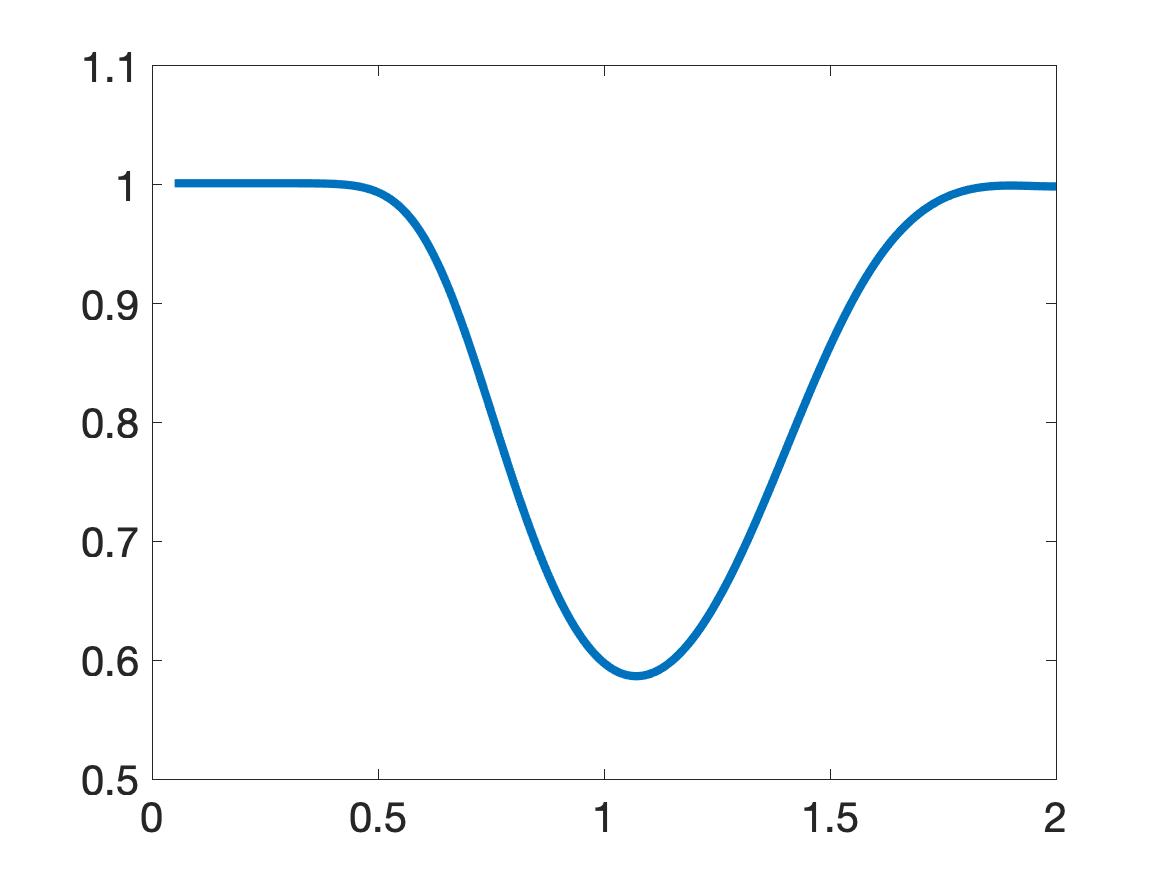
Next, we preprocess the data as follows. First, we first use a lower envelop (built in Matlab) to bound the data. We then truncate the data that is not in a small interval centered at the global minimizer of the data, see [30, Section 7.1] for the choice of this small interval. But in the case of the plastic cylinder we use the upper envelop. The choice of the upper or lower envelopes is as follows. We look at the function and find the three extrema with largest absolute values. If the middle extremal value among these three is a minimum, then we bound the data by a lower envelop. Otherwise, we use an upper envelop. See [30, Section 7.1] for more details and the reason of this choice. In particular, Figures 4a, 4b, 4d, 5a, 5b, 5d, 5e, 5g, 5h of [30] provide illustrations. Likewise, our Figures 5 displays computed functions for our five targets. The computed dielectric constants defined in (11.3) by Algorithm 1 is listed in Table 1.
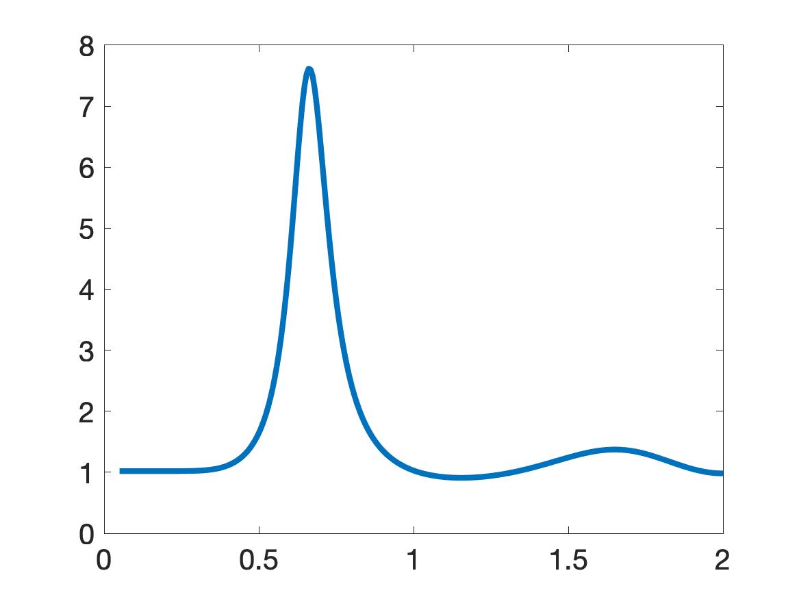
| Target | computed | computed | True | ||
|---|---|---|---|---|---|
| Bush | 1 | 7.62 | 1 | 10.99 | |
| Wood stake | 1 | 2.01 | 1 | 2.26 | |
| Metal box | 4 | 4.00 | |||
| Metal cylinder | 4 | 4.01 | |||
| Plastic cylinder | 4 | 0.59 |
The true values of dielectric constants of our targets were not measured in the experiment. Therefore, we compare our computed values with the published ones. The published values of the dielectric constants of our targets are listed in the last column of Table 1. They can be found on the website of Honeywell (Table of dielectric constants, https://goo.gl/kAxtzB). Also, see [9] for the experimentally measured range of the dielectric constants of vegetation samples, which we assume have the same range as the dielectric constant of bush. In the table of dielectric constants of Honeywell as well as in [9], any dielectric constant is not a number. Rather, each dielectric constant of these references is given within a certain interval. As to the metallic targets, it was established in [35] that they have the so-called “apparent” dielectric constant whose values are in the interval
Conclusion. It is clear from Table 1 that our computed dielectric constants are consistent with the intervals of published ones. Therefore, our results for experimental data are satisfactory.
Remark 11.1 (Speed of computations).
Our experimental data are sparse. The size of the data in time is , which is a lot smaller than that in the dense simulated data (). Therefore, the speed of computations is much faster than for the case of simulated data of section 10. Thus, all results of this section were computed in real time on the same computer (MacBook Pro 2019 with 2.6 GHz processor and 6 Intel i7 cores).
12 Concluding Remarks
We have developed a new globally convergent numerical method for a 1-D Coefficient Inverse Problem with backscattering data for the wave-like PDE (2.3). This is the second generation of the above cited convexification method of our research group. The main novelty here is that, rather than minimizing a globally strictly convex weighted cost functional arising in the convexification, we solve on each iterative step a linear boundary value problem. This is done using the so-called Carleman Quasi-Reversibility Method. Just like in the convexification, the key element of the technique of this paper, on which our convergence analysis is based, is the presence of the Carleman Weight Function in each quadratic functional which we minimize. The convergence estimate is similar to the key estimate of the classical contraction mapping principle. The latter explains the title of this paper. We have proven a global convergence theorem of our method. Our numerical results for computationally simulated data demonstrate high reconstruction accuracies in the presence of 5% random noise in the data.
Furthermore, our numerical results for experimentally collected data have satisfactory accuracy via providing values of computed dielectric constants of explosive-like targets within their published ranges.
A practically important observation here is that our computations for experimental data were performed in real time.
Acknowledgement
The effort of TTL, MVK and LHN was supported by US Army Research Laboratory and US Army Research Office grant W911NF-19-1-0044.
References
- [1] A. B. Bakushinskii, M. V. Klibanov, and N. A. Koshev. Carleman weight functions for a globally convergent numerical method for ill-posed Cauchy problems for some quasilinear PDEs. Nonlinear Anal. Real World Appl., 34:201–224, 2017.
- [2] L. Baudouin, M. de Buhan, and S. Ervedoza. Convergent algorithm based on Carleman estimates for the recovery of a potential in the wave equation. SIAM J. Nummer. Anal., 55:1578–1613, 2017.
- [3] L. Baudouin, M. de Buhan, S. Ervedoza, and A. Osses. Carleman-based reconstruction algorithm for the waves. SIAM Journal on Numerical Analysis, 59(2):998–1039, 2021.
- [4] L. Beilina and M. V. Klibanov. Approximate Global Convergence and Adaptivity for Coefficient Inverse Problems. Springer, New York, 2012.
- [5] M. Bellassoued and M. Yamamoto. Carleman Estimates and Applications to Inverse Problems for Hyperbolic Systems. Springer, Japan, 2017.
- [6] A. L. Bukhgeim and M. V. Klibanov. Uniqueness in the large of a class of multidimensional inverse problems. Soviet Math. Doklady, 17:244–247, 1981.
- [7] T. Carleman. Sur un probleme d’unicit e pur les systeé mes d’equations aux dériveés partielles à deux varibales indépendantes. Ark. Mat. Astr. Fys., 26B:1–9, 1939.
- [8] G. Chavent. Nonlinear Least Squares for Inverse Problems: Theoretical Foundations and Step-by-Step Guide for Applications, Scientic Computation. Springer, New York, 2009.
- [9] H. T. Chuah, K. Y. Lee, and T. W. Lau. Dielectric constants of rubber and oil palm leaf samples at X-band. IEEE Trans. Geosci. Remote Sens, 33, 221–223, 1995.
- [10] M. de Hoop, P. Kepley, and L. Oksanen. Recovery of a smooth metric via wave field and coordinate transformation reconstruction. SIAM J. Appl. Math., 78:1931–1953, 2018.
- [11] A. V. Goncharsky and S. Y. Romanov. Iterative methods for solving coefficient inverse problems of wave tomography in models with attenuation. Inverse Problems, 33:025003, 2017.
- [12] V. Goncharsky and S. Y. Romanov. A method of solving the coefficient inverse problems of wave tomography. Comput. Math. Appl., 77:967–980, 2019.
- [13] A.L. Karchevsky, M.V. Klibanov, L. Nguyen, N. Pantong, and A. Sullivan. The Krein method and the globally convergent method for experimental data. Applied Numerical Mathematics, 74:111–127, 2013.
- [14] V. A. Khoa, G. W. Bidney, M. V. Klibanov, L. H. Nguyen, L. Nguyen, A. Sullivan, and V. N. Astratov. Convexification and experimental data for a 3D inverse scattering problem with the moving point source. Inverse Problems, 36:085007, 2020.
- [15] V. A. Khoa, G. W. Bidney, M. V. Klibanov, L. H. Nguyen, L. Nguyen, A. Sullivan, and V. N. Astratov. An inverse problem of a simultaneous reconstruction of the dielectric constant and conductivity from experimental backscattering data. Inverse Problems in Science and Engineering, 29(5):712–735, 2021.
- [16] V. A. Khoa, M. V. Klibanov, and L. H. Nguyen. Convexification for a 3D inverse scattering problem with the moving point source. SIAM J. Imaging Sci., 13(2):871–904, 2020.
- [17] M. V. Klibanov. Inverse problems and Carleman estimates. Inverse Problems, 8:575–596, 1992.
- [18] M. V. Klibanov. Carleman estimates for global uniqueness, stability and numerical methods for coefficient inverse problems. J. Inverse and Ill-Posed Problems, 21:477–560, 2013.
- [19] M. V. Klibanov. Carleman estimates for the regularization of ill-posed Cauchy problems. Applied Numerical Mathematics, 94:46–74, 2015.
- [20] M. V. Klibanov and O. V. Ioussoupova. Uniform strict convexity of a cost functional for three-dimensional inverse scattering problem. SIAM J. Math. Anal., 26:147–179, 1995.
- [21] M. V. Klibanov. Global convexity in a three-dimensional inverse acoustic problem. SIAM J. Math. Anal., 28:1371–1388, 1997.
- [22] M. V. Klibanov and A. Timonov. Carleman Estimates for Coefficient Inverse Problems and Numerical Applications. Inverse and Ill-Posed Problems Series. VSP, Utrecht, 2004.
- [23] M. V. Klibanov, L. H. Nguyen, A. Sullivan, and L. Nguyen. A globally convergent numerical method for a 1-d inverse medium problem with experimental data. Inverse Problems and Imaging, 10:1057–1085, 2016.
- [24] M. V. Klibanov, A. E. Kolesov, L. Nguyen, and A. Sullivan. Globally strictly convex cost functional for a 1-D inverse medium scattering problem with experimental data. SIAM J. Appl. Math., 77:1733–1755, 2017.
- [25] M. V. Klibanov, A. E. Kolesov, L. Nguyen, and A. Sullivan. A new version of the convexification method for a 1-D coefficient inverse problem with experimental data. Inverse Problems, 34:35005, 2018.
- [26] M. V. Klibanov, A. E. Kolesov, and D-L. Nguyen. Convexification method for an inverse scattering problem and its performance for experimental backscatter data for buried targets. SIAM J. Imaging Sci., 12:576–603, 2019.
- [27] M. V. Klibanov, J. Li, and W. Zhang. Convexification of electrical impedance tomography with restricted Dirichlet-to-Neumann map data. Inverse Problems, 35:035005, 2019.
- [28] M. V. Klibanov, Z. Li, and W. Zhang. Convexification for the inversion of a time dependent wave front in a heterogeneous medium. SIAM J. Appl. Math., 79:1722–1747, 2019.
- [29] M. V. Klibanov, J. Li, and W. Zhang. Convexification for an inverse parabolic problem. Inverse Problems, 36:085008, 2020.
- [30] M. V. Klibanov, T. T. Le, L. H. Nguyen, A. Sullivan, and L. Nguyen. Convexification-based globally convergent numerical method for a 1D coefficient inverse problem with experimental data. preprint, Arxiv:2104.11392, 2021.
- [31] M. V. Klibanov and J. Li. Inverse Problems and Carleman Estimates: Global Uniqueness, Global Convergence and Experimental Data. , De Gruyter, 2021.
- [32] M. V. Klibanov, A. V. Smirnov, V. A. Khoa, A. Sullivan, and L. Nguyen. Through-the-wall nonlinear SAR imaging. IEEE Transactions on Geoscience and Remote Sensing, 59: 7474-7486, 2021.
- [33] M. V. Klibanov, V. A. Khoa, A. V. Smirnov, L. H. Nguyen, G. W. Bidney, L. Nguyen, A. Sullivan, and V. N. Astratov. Convexification inversion method for nonlinear SAR imaging with experimentally collected data. to appear in J. Applied and Industrial Mathematics, see also Arxiv:2103.10431, 2021.
- [34] J. Korpela, M. Lassas, and L. Oksanen. Regularization strategy for an inverse problem for a dimensional wave equation. Inverse Problems, 32:065001, 2016.
- [35] A. Kuzhuget, L. Beilina, M.V. Klibanov, A. Sullivan, Lam Nguyen, and M. A. Fiddy. Blind backscattering experimental data collected in the field and an approximately globally convergent inverse algorithm. Inverse Problems, 28:095007, 2012.
- [36] A. V. Kuzhuget, L. Beilina, M. V. Klibanov, A. Sullivan, L. Nguyen, and M. A. Fiddy. Quantitative image recovery from measured blind backscattered data using a globally convergent inverse method. IEEE Trans. Geosci. Remote Sens, 51:2937–2948, 2013.
- [37] R. Lattès and J. L. Lions. The Method of Quasireversibility: Applications to Partial Differential Equations. Elsevier, New York, 1969.
- [38] M. M. Lavrent’ev, V. G. Romanov, and S. P. Shishatskiĭ. Ill-Posed Problems of Mathematical Physics and Analysis. Translations of Mathematical Monographs. AMS, Providence: RI, 1986.
- [39] T. T. Le and L. H. Nguyen. A convergent numerical method to recover the initial condition of nonlinear parabolic equations from lateral Cauchy data. Journal of Inverse and Ill-posed Problems, DOI: https://doi.org/10.1515/jiip-2020-0028, 2020.
- [40] T. T. Le and L. H. Nguyen. The gradient descent method for the convexification to solve boundary value problems of quasi-linear PDEs and a coefficient inverse problem. preprint Arxiv:2103.04159, 2021.
- [41] B. M. Levitan. Inverse Sturm–Liouville Problems. VSP, Utrecht, 1987.
- [42] M. Minoux. Mathematical Programming: Theory and Algorithms. John Wiley & Sons, New York, 1986.
- [43] L. H. Nguyen. A new algorithm to determine the creation or depletion term of parabolic equations from boundary measurements. Computers and Mathematics with Applications, 80:2135–2149, 2020.
- [44] L. H. Nguyen and M. V. Klibanov. Carleman estimates and the contraction principle for an inverse source problem for nonlinear hyperbolic equations. preprint arXiv:2108.03500, 2021.
- [45] L. H. Nguyen and M. V. Klibanov. Carleman estimates and the contraction principle for an inversesource problem for nonlinear hyperbolic equations. preprint arXix:2108.03500v3, 2021.
- [46] N. Nguyen, D. Wong, M. Ressler, F. Koenig, Stanton B., G. Smith, J. Sichina, and K. Kappra. Obstacle avolidance and concealed target detection using the Army Research Lab ultra-wideband synchronous impulse Reconstruction (UWB SIRE) forward imaging radar. Proc. SPIE, 6553:65530H (1)–65530H (8), 2007.
- [47] P. M. Nguyen and L. H. Nguyen. A numerical method for an inverse source problem for parabolic equations and its application to a coefficient inverse problem. Journal of Inverse and Ill-posed Problems, 38:232–339, 2020.
- [48] V.G. Romanov. Inverse Problems of Mathematical Physics, VNU Press, 1986.
- [49] J. A. Scales, M. L. Smith, and T. L. Fischer. Global optimization methods for multimodal inverse problems. J. Computational Physics, 103:258–268, 1992.
- [50] A. V. Smirnov, M. V. Klibanov, and L. H. Nguyen. Convexification for a 1D hyperbolic coefficient inverse problem with single measurement data. Inverse Probl. Imaging, 14(5):913–938, 2020.
- [51] A. V. Smirnov, M. V. Klibanov, A. Sullivan, and L. Nguyen. Convexifcation for an inverse problem for a 1D wave equation with experimental data. Inverse Problems, 36:095008, 2020.
- [52] A. N. Tikhonov, A. Goncharsky, V. V. Stepanov, and A. G. Yagola. Numerical Methods for the Solution of Ill-Posed Problems. Kluwer Academic Publishers Group, Dordrecht, 1995.
- [53] M. Yamamoto. Carleman estimates for parabolic equations. Topical Review. Inverse Problems, 25:123013, 2009.