CASCADED ALL-PASS FILTERS WITH RANDOMIZED CENTER FREQUENCIES AND PHASE POLARITY FOR
ACOUSTIC AND SPEECH MEASUREMENT AND
DATA AUGMENTATION
Abstract
We introduce a new member of TSP (Time Stretched Pulse) for acoustic and speech measurement infrastructure, based on a simple all-pass filter and systematic randomization. This new infrastructure fundamentally upgrades our previous measurement procedure, which enables simultaneous measurement of multiple attributes, including non-linear ones without requiring extra filtering nor post-processing. Our new proposal establishes a theoretically solid, flexible, and extensible foundation in acoustic measurement. Moreover, it is general enough to provide versatile research tools for other fields, such as biological signal analysis. We illustrate using acoustic measurements and data augmentation as representative examples among various prospective applications. We open-sourced MATLAB implementation. It consists of an interactive and real-time acoustic tool, MATLAB functions, and supporting materials.
Index Terms— Time stretched pulse, all-pass filter, distribution shaping, simultaneous measurement, data augmentation.
1 Introduction
There is a vast knowledge gap in our auditory processing principle connecting waveform and perception, especially in a fine time scale. The signal family we propose may provide the key to fill the gap.
Phenomena that illustrates the gap are: A broad class of sounds is perceived identical, although they are entirely different in sampled value levels at the audio sampling rate. Waveform modification by group delay within 0.5 ms is not detectable[1]. The detection threshold of a brief noise burst varies 20 dB depending on the burst location inside one pitch period[2]. Group delay compensation of the traveling wave propagation on the basilar membrane enhances the evoked potential response while reduces “compactness” of the unit pulse, and the unit pulse without group delay modification yields the most “compactness”[3]. These phenomena motivated the first author to discard the phase information of speech sounds in STRAIGHT[4]. The invention of FVN (Frequency domain variant of Velvet Noise)[5] is the most recent example driven by this motivation. We designed it for the excitation source of synthetic speech.
Accidentally, we found that FVN provides powerful tools for assessing acoustic systems[6]. FVN is a new member of TSP (Time Stretched Pulse)[7, 8, 9, 10, 11, 12] in a broad sense. Well-known TSP members are pseudo-random noise (PN) and swept-sine (SS) signals. They provide an essential infrastructure of acoustic measurement and assessment[7, 8, 13, 14, 12, 15]. It is crucial to acquire reusable speech materials[16, 17] and present sound stimuli to participants of subjective tests using adequately prepared sound devices and the environment. FVN also added new functionality to assessment tools[6].
Concerning the gap, FVN provides a means to augment acoustic data for end-to-end DL-based applications[18]. Systematic group delay modification of the original signal can generate many perceptually identical signals. Eventually, the end-to-end approach may yield latent variables that embody still mysterious human auditory processing principles. If it would provide a clue for uncovering the mystery, it is a desirable consequence of our original motivation lead.
Unfortunately, FVN is not theoretically solid enough to support rigorous scientific and engineering research. FVN is a mixture of many heuristics that started from time and frequency axes exchange of the original velvet noise[19, 20]. FVN design procedure modifies the phase of the transfer function of a unit pulse using a weighted sum of six-term cosine series[21]. This procedure has many tuning parameters without solid theoretical backgrounds. The procedure modifies the phase to manipulate the actual manipulation target, the group delay. The assignment rule of phase manipulation functions, a modified copy of the original velvet noise, may not be the best.
This article proposes another member of TSP called CAPRICEP111 Cascaded All-Pass filters with RandomIzed CEnter frequencies and Phase polarities. CAPRICEP removes all these difficulties and expands FVN’s functionality. IIR all-pass filter, a starting building block of CAPRICEP, has only one tuning parameter, the root’s proximity to the unit circle. IIR all-pass filter has a unique phase function shape. It provides means to directly design the group delay instead of indirectly design using the phase. Built-in numerical optimization assures that the generated CAPRICEP is optimum.
The significant contribution of this article is the proposal of CAPRICEP. The following section provides the derivation of CAPRICEP followed by a brief introduction of the simultaneous measurement method of multiple responses. The derivation of this simultaneous measurement method is a replication of the FVN-based method’s[6]. CAPRICEP adds flexibility and extended functionality because of its building block, all-pass filter.
Then, we introduce two representative examples to illustrate the possibilities of CAPRICEP-based methods. First is an interactive and real-time acoustic measurement tool. The tool is for measuring sound acquisition and sound reproduction systems. Proper assessment based on these measurements is crucial for preparing and evaluating sound materials. The second example concerns the knowledge gap. Using a set of unit-CAPRICEPs as a filter-bank, it provides perceptually indistinguishable sounds from original recordings. It works as a data augmentation device for the end-to-end approach[18]. Finally, we review other related works and other possible applications. We found that CAPRICEP enables a new approach for investigating the role of auditory perception while speaking and singing[22, 23, 24, 25, 26].
2 Proposed TSP: CAPRICEP
An all-pass filter is a filter whose gain transfer function is a frequency-independent constant. Other than the trivial solution, a unit impulse, an all-pass filter has an impulse response that temporally spreads. It is a member of TSP signals, in a broad sense. Cascaded all-pass filters also yield an all-pass filter. By introducing a systematic procedure, we can design useful attributes to the yielded filter’s impulse response.
The design goal of the response is as follows: a) The waveform is temporally localized, b) It has many degrees of freedom in designing the waveform, and consequently c) Cross-correlation between different generated waveform is close to zero. In other words, we want noise bursts with a completely flat (frequency-independent) power spectrum. CAPRICEP fulfilled the goal.
2.1 Building block: all-pass filter
Let us start from its building block. The following equation defines the transfer function of a simple discrete-time all-pass filter, characterized by the center frequency and the bandwidth [27].
| (1) | ||||
| (2) |
where represents the sampling frequency and . A term represents the complex conjugate of . By cascading these building blocks also yields an all-pass filter. Its inverse z-transform provides an impulse response. We call the impulse response unit-CAPRICEP afterward.
2.2 Cascaded all-pass filters: CAPRICEP
The transfer function of the cascaded all-pass filters is the product of constituent transfer function .
| (3) |
where represents the total number of the cascaded filters. A systematic procedure determines each center frequency using two set of random numbers and . We introduce random numbers because each pole corresponds to a damped sinusoid. Intuitively speaking, the sum of many sinusoids with the same amplitude with the random phase yields items behave like samples from normal distribution[28]. We hope frequency randomization yields noise-like behavior of the impulse response of .
The following equation is an implementation of the systematic procedure of filter assignment.
| (4) |
where represents the average interval between aligned center frequencies (i.e. ). The random number has the value and with equal probability. Note that makes anti-causal and makes its impulse response time-reversed. This randomization is for design flexibility described in the next section. Without introducing , the response is causal and does not provide flexible design.
The random number obeys a probability density distribution function (pdf) defined on . We do not randomize directly. Instead, we randomized the frequency interval between neighboring all-pass filters. References[19, 20] reported simple random allocation does not yield well-behaved velvet noise222 They named the noise “velvet noise” because the noise sounds smoother than Gaussian white noise. Simple random allocation destroyed the smoothness[19, 20]. . Intuitively speaking, the original velvet noise and FVN use the triangular pdf for interval distribution. They also use the additional constraint, fixed-width partitioning of the time axes. This fixed-width partitioning forced us to introduce non-linear frequency axis warping for shaping temporal distribution[5].
We introduce the Beta distribution for because it is a simple adjustable distribution having two design parameters. The following is the definition of the Beta distribution.
| (5) |
where is Gamma function. When , seamlessly deforms from concave to convex via uniform distribution with .
For (Eq. 2), we make it proportional to using a coefficient . In short, we set (at least for the first time). In summary, has three design parameters, , and . This additional parameter that FVN does not have enables us to design the shape of the waveform distribution. Let represent the impulse response of . It is unit-CAPRICEP.
2.3 Shaping waveform distribution of unit-CAPRICEP
Shaping waveform distribution is an optimization problem. Let us define the target shape on the discrete-time axis . We design the sample variance by minimizing a distance measure between and . We use Wasserstein distance[29] as the cost function to minimize because it is an energy allocation problem on the discrete-time axis, in the other words.
We selected the rectangular shape as the first target because it is suitable for making less-fluctuating test signals using periodic allocation (i.e. OLA: overlap and add) of unit-CAPRICEPs. We conducted several coarse multivariate optimizations before final optimization. It gave us the setting and . Then, we optimized the duration of the rectangle using a grid search.
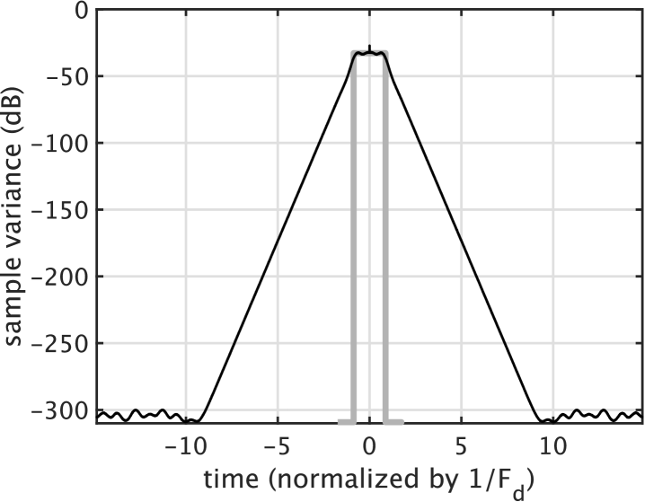
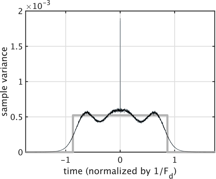
Figure 1 shows an example of shape design. The sample variance calculation used 5000 unit-CAPRICEPs. The optimized is 1.736 times of the nominal duration of . Note that the decay outside of the rectangle is exponential. The total number of cascaded filters is 1102 for Hz, Hz.
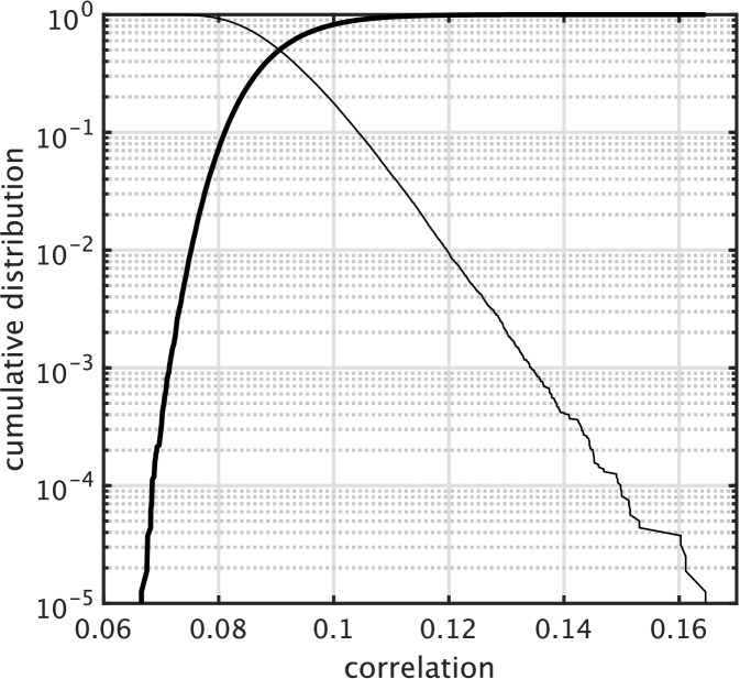
Left plot of Fig. 2 shows the distribution of the maximum cross correlation (absolute value) of pairs of different unit-CAPRICEPs. The thick line shows probability where represents the maximum cross correlation and represents the threshold correlation value shown in the horizontal axis. The thin line shows . The median of the distribution is 0.0905 and close to zero.
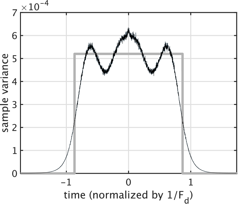
Another useful target shape is the raised cosine because OLA with 50% overlap provides a constant level. Cascading a short (0.5 ms) raised cosine-shaped unit-CAPRICEP and the rectangular one yielded the shape shown in the right plot of Fig. 2. The outstanding spike at the center shown in Fig. 1 disappears. This composite shape is appropriate for acoustic measurement applications.
2.4 Summary of this section: goal and the result
CAPRICEP fulfilled the design goal as follows: a) Using IIR all-pass filter as the building block made the decaying exponential that enables well-behaving localization (section 2.1). b) Cascading many filters provides many degrees of freedom (section 2.2 and 2.3). c) Many degrees of freedom made cross-correlation between different unit-CAPRICEPs close to zero (section 2.3).
Note that making frequency-dependent is straightforward for CAPRICEP, while complicated and indirect for FVN[5]. There is much additional flexibility in design using and , which are fix-valued in the current implementation.
3 Simultaneous measurement
Systematic allocation of unit-FVNs enabled simultaneous measurement of the linear time-invariant, the non-linear time-invariant responses and random and time-varying components[6]. Replacing FVN with CAPRICEP also enables a similar simultaneous measurement. The following is a brief outline of the procedure in[6].
3.1 Four CAPRICEP sequences and response measurement
A set of four periodic sequences made from unit-CAPRICEPs enables the simultaneous measurement. Define a weight matrix , which consists of four orthogonal binary rows shown below.
| (10) | ||||
| (11) |
The following equation defines the -th CAPRICEP sequence . This procedure is a periodic OLA.
| (12) |
where represents the -th element of . represents the number of repetitions. Note that 8 is the number of columns of .
3.2 Pulse recovery
Make a test by adding the first three CAPRICEP sequences. Convolution of the test signals and the time-reversed unit-CAPRICEP yields compressed signal . They consist of recovered pulses corresponding to repetitions. Since a set of unit-CAPRICEPs are not strictly orthogonal, correlations remain.
| (13) |
where “” represents the convolution operation.
3.3 Orthogonalization
The inner product of and of (11) is zero when . Periodic time shift and averaging using the binary weights in remove these cross-correlations. The following equation yields the orthogonalized signal .
| (14) |
where is the length of the weight vectors . The notation represents cyclic indexing between 1 and 8.
3.4 Synchronous averaging for unit impulse recovery
Synchronous averaging given below yields the unit impulse response. It also reduces the effect of random fluctuation of the signal.
| (15) |
where , and the symbol represents the region where cross-correlation is effectively vanished. The function yields the number of pulses separated by and located inside the region. Then, further averaging the first three responses provides the final averaged response .
| (16) |
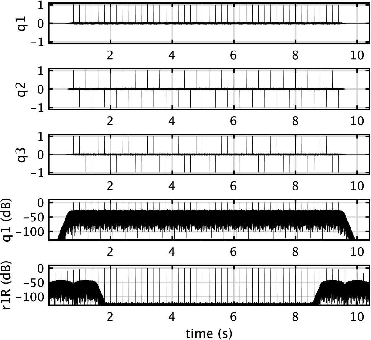
Figure 3 shows examples to illustrates these procedures. This example uses CAPRICEP designed to have the equivalent rectangular duration s. We truncated the length of CAPRICEP 0.8 s for implementation using FFT-based fast convolution. IIR-based implementation requires a two-pass procedure consisting of time axis reversal, which is not relevant for real-time applications. The top three plots of Fig. 3 show the recovered signals (. The fourth plot shows using dB scale. The background noise around 45 dB is the result of the cross-correlation between unit-CAPRICEPs. The bottom plot shows the orthogonalized signal using the dB scale. Note that the orthogonalization procedure removes components due to cross-correlation between unit-CAPRICEPs.
3.5 Measuring deviations from linear time-invariant systems
The orthogonalized signal using the fourth unit-CAPRICEP does not consist of components in the test signal . Therefore, consists of the background noise, the effects of temporal variation in the response, and randomly generated non-linear time-variant response.
The consecutive eight repetition segments provide the eight possible combinations of three unit-CAPRICEPs’ polarities. The averaged response is the average of all these combinations, deviations from this average consists of the non-linear time-invariant responses (and the random component mentioned above). Detailed derivation in [6] provides the procedure of the simultaneous measurement and simulation tests quantitatively validated the procedure using FVN. This derivation holds for CAPRICEP because FVN and CAPRICEP are members of TSP. We conducted the same simulation by replacing FVNs with CAPRICEPs. The results using CAPRICEP also validated the procedure.
4 Application and discussion
We introduce two examples of CAPRICEP’s application, an interactive acoustic measurement tool and data augmentation.
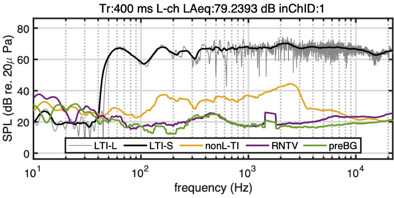
Figure 4 shows an example of simultaneous multiple attribute measurement. Distance between the microphone and the powered loudspeaker was 50 cm located in a home office. We used an interactive and real-time acoustic measurement tool[30] based on CAPRICEP, which is a substantial upgrade of our FVN-based tool[6].
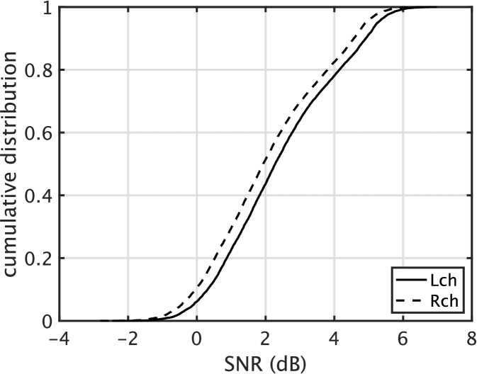
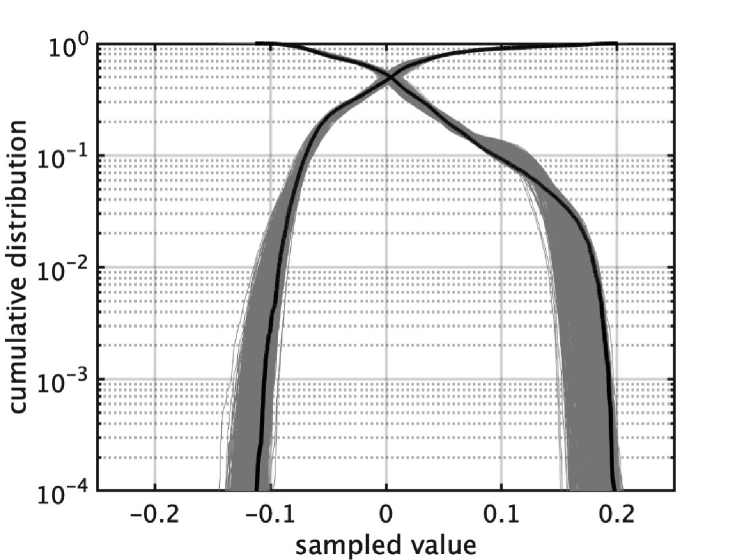
The end-to-end approach requires an enormous amount of training data[18]. When data is scarce, such as low-resource languages, data augmentation applies. Using many unit-CAPRICEPs provides arbitrarily many perceptually identical samples from a single original sound material. Figure 5 shows two examples. Left uses music data excerpted from[31]. Despite this low-SNR distribution, the impression of the filtered sounds is identical to the original. No impression of noise. Right shows a voice (Japanese vowel /e/) example[32]. Filtering by unit-CAPRICEPs modifies the waveform. The original asymmetric distribution (thick black lines) turned into less asymmetric distribution (gray 2000 lines) by filtering. The filtered signals sound perceptually identical despite that they are significantly different in the waveform. Sample files are in the first author’s GitHub repository [30].
TSP-based methods[7, 8, 9, 10, 11] are commonly used in acoustic measurement and appropriate for measuring linear time-invariant responses. However, they need extra-equipment or inspection by experts for analyzing non-linear responses and inter-modulation distortion[13, 15, 14, 12]. FVN solved this problem by proposing a simultaneous measurement method that does not require extra-equipment nor experts’ inspection[6]. The proposed CAPRICEP revised the FVN-based method with a theoretically solid and more flexible foundation. The proposed method is general enough for investigating systems with inherent non-linear and temporal variability, biological systems. We are planning to apply the CAPRICEP-based method for investigating the auditory-to-speech production mechanism[22, 23, 24, 25, 26].
5 conclusion
We proposed a new member of TSP called CAPRICEP. A unit-CAPRICEP is an impulse response of an all-pass filter with high degrees of freedom in design and provides a theoretically sound infrastructure for acoustic measurement and assessment. CAPRICEP opens vast application possibilities spanning from acoustic measurement, speech synthesis, signal processing for biological systems, and data augmentation for the end-to-end approach of sound-related applications. It also provides an essential key for fundamental research of human auditory perception principles. We made the CAPRICEP-based interactive and real-time acoustic measurement tools and related MATLAB functions open-source in the first author’s GitHub repository[30].
References
- [1] J. Blauert and P. Laws, “Group delay distortions in electroacoustical systems,” J. Acoust. Soc. Am., vol. 63, no. 5, pp. 1478–1483, 1978.
- [2] J. Skoglund and W. B. Kleijn, “On time-frequency masking in voiced speech,” IEEE Trans. Speech Audio Process., vol. 8, no. 4, pp. 361–369, 2000.
- [3] S. Uppenkamp, S. Fobel, and R. D. Patterson, “The effects of temporal asymmetry on the detection and perception of short chirps,” Hear. Res., vol. 158, no. 1, pp. 71–83, 2001.
- [4] H. Kawahara, I. Masuda-Katsuse, and A. de Cheveigne, “Restructuring speech representations using a pitch-adaptive time-frequency smoothing and an instantaneous-frequency-based F0 extraction,” Speech Commun., vol. 27, no. 3-4, pp. 187–207, 1999.
- [5] H. Kawahara, K. Sakakibara, M. Morise, H. Banno, T. Toda, and T. Irino, “Frequency domain variants of velvet noise and their application to speech processing and synthesis,” in Proc. Interspeech 2018, Hyderabad, India, 2018, pp. 2027–2031.
- [6] H. Kawahara, K. Sakakibara, M. Mizumachi, M. Morise, and H. Banno, “Simultaneous measurement of time-invariant linear and nonlinear, and random and extra responses using frequency domain variant of velvet noise,” arXiv:2008.02439, 2020, (Accepted for APSIPA ASC 2020).
- [7] M. R. Schroeder, “Integrated-impulse method measuring sound decay without using impulses,” J. Acoust. Soc. Am., vol. 66, no. 2, pp. 497–500, 1979.
- [8] N. Aoshima, “Computer-generated pulse signal applied for sound measurement,” J. Acoust. Soc. Am., vol. 69, no. 5, pp. 1484–1488, 1981.
- [9] S. Müller and P. Massarani, “Transfer-function measurement with sweeps,” J. Audio Eng. Soc., vol. 49, no. 6, pp. 443–471, 2001.
- [10] H. Ochiai and Y. Kaneda, “A recursive adaptive method of impulse response measurement with constant SNR over target frequency band,” J. Audio Eng. Soc, vol. 61, no. 9, pp. 647–655, 2013.
- [11] P. Guidorzi, L. Barbaresi, D. D’Orazio, and M. Garai, “Impulse responses measured with MLS or Swept-Sine signals applied to architectural acoustics: an in-depth analysis of the two methods and some case studies of measurements inside theaters,” Energy Procedia, vol. 78, pp. 1611–1616, 2015.
- [12] P. Burrascano, S. Laureti, M. Ricci, A. Terenzi, S. Cecchi, S. Spinsante, and F. Piazza, “A swept-sine pulse compression procedure for an effective measurement of intermodulation distortion,” IEEE Trans. Instrum. Meas., vol. 69, no. 4, pp. 1708–1719, 2019.
- [13] C. Dunn and M. J. Hawksford, “Distortion immunity of MLS-derived impulse response measurements,” J. Audio Eng. Soc., vol. 41, no. 5, pp. 314–335, 1993.
- [14] G.-B. Stan, J.-J. Embrechts, and D. Archambeau, “Comparison of different impulse response measurement techniques,” J. Audio Eng. Soc., vol. 50, no. 4, pp. 249–262, 2002.
- [15] A. Farina, “Simultaneous measurement of impulse response and distortion with a swept-sine technique,” in Audio Eng. Soc. Conv. 108. AES, 2000.
- [16] J. G. Švec and S. Granqvist, “Guidelines for selecting microphones for human voice production research,” Am. J. Speech-Lang. Pathol., vol. 19, no. 4, pp. 356–368, 2010.
- [17] R. R. Patel, S. N. Awan, J. Barkmeier-Kraemer, M. Courey, D. Deliyski, T. Eadie, D. Paul, J. G. Švec, and R. Hillman, “Recommended protocols for instrumental assessment of voice: American speech-language-hearing association expert panel to develop a protocol for instrumental assessment of vocal function,” Am. J. Speech-Lang. Pathol., vol. 27, no. 3, pp. 887–905, 2018.
- [18] H. Purwins, B. Li, T. Virtanen, J. Schlüter, S. Chang, and T. Sainath, “Deep learning for audio signal processing,” IEEE J. Sel. Top. Signal Process., vol. 13, no. 2, pp. 206–219, 2019.
- [19] H. Järveläinen and M. Karjalainen, “Reverberation modeling using velvet noise,” in Proc. AES 30th Int. Conf., 2007, pp. 15–17.
- [20] V. Välimäki, H. M. Lehtonen, and M. Takanen, “A perceptual study on velvet noise and its variants at different pulse densities,” IEEE Trans. Audio, Speech, Lang. Process., vol. 21, no. 7, pp. 1481–1488, July 2013.
- [21] H. Kawahara, K. Sakakibara, M. Morise, H. Banno, T. Toda, and T. Irino, “A new cosine series antialiasing function and its application to aliasing-free glottal source models for speech and singing synthesis,” in Proc. Interspeech 2017, Stocholm, August 2017, pp. 1358–1362.
- [22] H. Kawahara, “Interactions between speech production and perception under auditory feedback perturbations on fundamental frequencies,” J. Acoust. Soc. Jpn. (E), vol. 15, no. 3, pp. 201–202, 1994.
- [23] Hideki Kawahara, Hiroko Kato, and J. C. Williams, “Effects of auditory feedback on F0 trajectory generation,” in Proc. ICSLP 96, 1996, pp. 287–290.
- [24] Jason A. Tourville, Kevin J. Reilly, and Frank H. Guenther, “Neural mechanisms underlying auditory feedback control of speech,” NeuroImage, vol. 39, no. 3, pp. 1429 – 1443, 2008.
- [25] E. F. Chang, C. A. Niziolek, R. T. Knight, S. S. Nagarajan, and J. F. Houde, “Human cortical sensorimotor network underlying feedback control of vocal pitch,” Proc. Natl. Acad. Sci. U.S.A., vol. 110, no. 7, pp. 2653–2658, 2013.
- [26] J. M. Zarate, “The neural control of singing,” Front. Hum. Neurosci., vol. 7, pp. 237, 2013.
- [27] A. V. Oppenheim and R. W. Schafer, Discrete-time signal processing: Pearson new International Edition, Pearson Higher Ed., 2013.
- [28] R. H. Lyon, “Statistics of combined sine waves,” J. Acoust. Soc. Am., vol. 48, no. 1B, pp. 145–149, 1970.
- [29] S. S. Vallender, “Calculation of the Wasserstein distance between probability distributions on the line,” Theory Probab. Appl., vol. 18, no. 4, pp. 784–786, 1974.
- [30] H. Kawahara, “CAPRICEP: An extended TSP that enables interactive and real-time measurement of the linear time–,” https://github.com/HidekiKawahara/CAPRICEP, 2021, (retrieved 13 Jan. 2021).
- [31] M. Goto, H. Hashiguchi, T. Nishimura, and R. Oka, “RWC music database: Popular, classical and jazz music databases,” in ISMIR, 2002, vol. 2, pp. 287–288.
- [32] I. Nakayama, “Comparative studies on vocal expression in Japanese traditional and western classical-style singing, using a common verse,” in Proc. ICA 2004, 2004, pp. 1295–1296.