Causal Conceptions of Fairness and their Consequences

Consider a population of individuals with observed covariates $X$, drawn i.i.d from a set $\mathcal{X}\subseteq\mathbb{R}^{n}$ with distribution $\mathcal{D}_{X}$. Further suppose that $A\in\mathcal{A}$ describes one or more discrete protected attributes, such as race or gender, which can be derived from $X$ (i.e., $A=\alpha(X)$ for some measurable function $\alpha$). Each individual is subject to a binary decision $D\in\{0,1\}$, determined by a (randomized) rule $d(x)\in[0,1]$, where $d(x)=\operatorname{Pr}(D=1\mid X=x)$ is the probability of receiving a positive decision.¹¹1That is, $D=\mathbb{1}_{U_{D}\leq d(X)}$, where $U_{D}$ is an independent uniform random variable. Given a budget $b$ with $0<b<1$, we require the decision rule to satisfy $\mathbb{E}[D]\leq b$, limiting the expected proportion of positive decisions.

In our running example, we imagine a population of applicants to a particular college, where $d$ denotes an admissions rule and $D$ indicates a binary admissions decision. To simplify our exposition, we assume all admitted students attend the school. In our setting, the covariates $X$ consist of an applicant’s test score and race $A\in\{a_{0},a_{1}\}$, where, for notational convenience, we consider two race groups. The budget $b$ bounds the expected proportion of admitted applicants.

Assuming there is no interference between units (Imbens & Rubin, 2015), we write $Y(1)$ and $Y(0)$ to denote potential outcomes of interest under each of the two possible binary decisions, where $Y=Y(D)$ is the realized outcome. We assume that $Y(1)$ and $Y(0)$ are drawn from a (possibly infinite) set $\mathcal{Y}\subseteq\mathbb{R}$, where $|\mathcal{Y}|>1$. In our admissions example, $Y$ is a binary variable that indicates college graduation (i.e., degree attainment), with $Y(1)$ and $Y(0)$ describing, respectively, whether an applicant would attain a college degree if admitted to or if rejected from the school we consider. Note that $Y(0)$ is not necessarily zero, as a rejected applicant may attend—and graduate from—a different university.

Given this setup, our goal is to construct decision policies $d$ that are broadly equitable, formalized in part by the causal notions of fairness described below. We focus on decisions that are made algorithmically, informed by historical data on applicants and subsequent outcomes.

A popular class of non-causal fairness definitions requires that error rates (e.g., false positive and false negative rates) are equal across protected groups (Hardt et al., 2016; Corbett-Davies & Goel, 2018). Causal analogues of these definitions have recently been proposed (Coston et al., 2020; Imai & Jiang, 2020; Imai et al., 2020; Mishler et al., 2021), which require various conditional independence conditions to hold between the potential outcomes, protected attributes, and decisions.²²2In the literature on causal fairness, there is at times ambiguity between “predictions” $\hat{Y}\in\{0,1\}$ of $Y$ and “decisions” $D\in\{0,1\}$. Following past work (e.g., Corbett-Davies et al., 2017; Kusner et al., 2017; Wang et al., 2019), here we focus exclusively on decisions, with predictions implicitly impacting decisions but not explicitly appearing in our definitions.

Below we list three representative examples of this class of fairness definitions: counterfactual predictive parity (Coston et al., 2020), counterfactual equalized odds (Mishler et al., 2021; Coston et al., 2020), and conditional principal fairness (Imai & Jiang, 2020).³³3Our subsequent analytical results extend in a straightforward manner to structurally similar variants of these definitions (e.g., requiring $Y(0)\mathchoice{\mathrel{\hbox to0.0pt{$\displaystyle\perp$\hss}\mkern 2.0mu{\displaystyle\perp}}}{\mathrel{\hbox to0.0pt{$\textstyle\perp$\hss}\mkern 2.0mu{\textstyle\perp}}}{\mathrel{\hbox to0.0pt{$\scriptstyle\perp$\hss}\mkern 2.0mu{\scriptstyle\perp}}}{\mathrel{\hbox to0.0pt{$\scriptscriptstyle\perp$\hss}\mkern 2.0mu{\scriptscriptstyle\perp}}}A\mid D=1$ or $D\mathchoice{\mathrel{\hbox to0.0pt{$\displaystyle\perp$\hss}\mkern 2.0mu{\displaystyle\perp}}}{\mathrel{\hbox to0.0pt{$\textstyle\perp$\hss}\mkern 2.0mu{\textstyle\perp}}}{\mathrel{\hbox to0.0pt{$\scriptstyle\perp$\hss}\mkern 2.0mu{\scriptstyle\perp}}}{\mathrel{\hbox to0.0pt{$\scriptscriptstyle\perp$\hss}\mkern 2.0mu{\scriptscriptstyle\perp}}}A\mid Y(0)$, variants of counterfactual predictive parity and counterfactual equalized odds, respectively).

In our college admissions example, counterfactual predictive parity means that among rejected applicants, the proportion who would have attained a college degree, had they been accepted, is equal across race groups.

In our running example, counterfactual equalized odds is satisfied when two conditions hold: (1) among applicants who would graduate if admitted (i.e., $Y(1)=1$), students are admitted at the same rate across race groups; and (2) among applicants who would not graduate if admitted (i.e., $Y(1)=0$), students are again admitted at the same rate across race groups.

In our example, conditional principal fairness means that “similar” applicants—where similarity is defined by the potential outcomes and covariates $W$—are admitted at the same rate across race groups.

An alternative causal framework for understanding fairness considers the effects of protected attributes on decisions (Wang et al., 2019; Kusner et al., 2017; Nabi & Shpitser, 2018; Wu et al., 2019; Mhasawade & Chunara, 2021; Kilbertus et al., 2017; Zhang & Bareinboim, 2018; Zhang et al., 2017). This approach, which can be understood as codifying the legal notion of disparate treatment (Goel et al., 2017; Zafar et al., 2017a), considers a decision rule to be fair if, at a high level, decisions for individuals are the same in “(a) the actual world and (b) a counterfactual world where the individual belonged to a different demographic group” (Kusner et al., 2017).⁴⁴4Conceptualizing a general causal effect of an immutable characteristic such as race or gender is rife with challenges, the greatest of which is expressed by the mantra, “no causation without manipulation” (Holland, 1986). In particular, analyzing race as a causal treatment requires one to specify what exactly is meant by “changing an individual’s race” from, for example, white to Black (Gaebler et al., 2022; Hu & Kohler-Hausmann, 2020). Such difficulties can sometimes be addressed by considering a change in the perception of race by a decision maker (Greiner & Rubin, 2011)—for instance, by changing the name listed on an employment application (Bertrand & Mullainathan, 2004), or by masking an individual’s appearance (Goldin & Rouse, 2000; Grogger & Ridgeway, 2006; Pierson et al., 2020; Chohlas-Wood et al., 2021b).

In contrast to “fairness through unawareness”—in which race and other protected attributes are barred from being an explicit input to a decision rule (cf. Dwork et al., 2012; Corbett-Davies & Goel, 2018)—the causal versions of this idea consider both the direct and indirect effects of protected attributes on decisions. For example, even if decisions only directly depend on test scores, race may indirectly impact decisions through its effects on educational opportunities, which in turn influence test scores. This idea can be formalized by requiring that decisions remain the same in expectation even if one’s protected characteristics are counterfactually altered, a condition known as counterfactual fairness  (Kusner et al., 2017).

In our running example, this means that for each group of observationally identical applicants (i.e., those with the same values of $X$, meaning identical race and test score), the proportion of students who are actually admitted is the same as the proportion who would be admitted if their race were counterfactually altered.

Counterfactual fairness aims to limit all direct and indirect effects of protected traits on decisions. In a generalization of this criterion—termed path-specific fairness (Chiappa, 2019; Nabi & Shpitser, 2018; Zhang et al., 2017; Wu et al., 2019)—one allows protected traits to influence decisions along certain causal paths but not others. For example, one may wish to allow the direct consideration of race by an admissions committee to implement an affirmative action policy, while also guarding against any indirect influence of race on admissions decisions that may stem from cultural biases in standardized tests (Williams, 1983).

The formal definition of path-specific fairness requires specifying a causal DAG describing relationships between attributes (both observed covariates and latent variables), decisions, and outcomes. In our running example of college admissions, we imagine that each individual’s observed covariates are the result of the process illustrated by the causal DAG in Figure 1. In this graph, an applicant’s race $A$ influences the educational opportunities $E$ available to them prior to college; and educational opportunities in turn influence an applicant’s level of college preparation, $M$, as well as their score on a standardized admissions test, $T$, such as the SAT. We assume the admissions committee only observes an applicant’s race and test score so that $X=(A,T)$, and makes their decision $D$ based on these attributes. Finally, whether or not an admitted student subsequently graduates (from any college), $Y$, is a function of both their preparation and whether they were admitted.⁵⁵5In practice, the racial composition of an admitted class may itself influence degree attainment, if, for example, diversity provides a net benefit to students (Page, 2007). Here, for simplicity, we avoid consideration of such peer effects.

To define path-specific fairness, we start by defining, for the decision $D$, path-specific counterfactuals, a general concept in causal DAGs (cf. Pearl, 2001). Suppose $\mathcal{G}=(\mathcal{V},\mathcal{U},\mathcal{F})$ is a causal model with nodes $\mathcal{V}$, exogenous variables $\mathcal{U}$, and structural equations $\mathcal{F}$ that define the value at each node $V_{j}$ as a function of its parents $\wp(V_{j})$ and its associated exogenous variable $U_{j}$. (See, for example, Pearl (2009a) for further details on causal DAGs.) Let $V_{1},\dots,V_{m}$ be a topological ordering of the nodes, meaning that $\wp(V_{j})\subseteq\{V_{1},\dots,V_{j-1}\}$ (i.e., the parents of each node appear in the ordering before the node itself). Let $\Pi$ denote a collection of paths from node $A$ to $D$. Now, for two possible values $a$ and $a^{\prime}$ for the variable $A$, the path-specific counterfactuals $D_{\Pi,a,a^{\prime}}$ for the decision $D$ are generated by traversing the list of nodes in topological order, propagating counterfactual values obtained by setting $A=a^{\prime}$ along paths in $\Pi$, and otherwise propagating values obtained by setting $A=a$. (In Algorithm 1 in the Appendix, we formally define path-specific counterfactuals for an arbitrary node—or collection of nodes—in the DAG.)

To see this idea in action, we work out an illustrative example, computing path-specific counterfactuals for the decision $D$ along the single path $\Pi=\{A\rightarrow E\rightarrow T\rightarrow D\}$ linking race to the admissions committee’s decision through test score, highlighted in red in Figure 1. In the system of equations below, the first column corresponds to draws $V^{*}$ for each node $V$ in the DAG, where we set $A$ to $a$, and then propagate that value as usual. The second column corresponds to draws $\overline{V}^{*}$ of path-specific counterfactuals, where we set $A$ to $a^{\prime}$, and then propagate the counterfactuals only along the path $A\rightarrow E\rightarrow T\rightarrow D$. In particular, the value for the test score $\overline{T}^{*}$ is computed using the value of $\overline{E}^{*}$ (since the edge $E\rightarrow T$ is on the specified path) and the value of $M^{*}$ (since the edge $M\rightarrow T$ is not on the path). As a result of this process, we obtain a draw $\overline{D}^{*}$ from the distribution of $D_{\Pi,a,a^{\prime}}$.

Path-specific fairness formalizes the intuition that the influence of a sensitive attribute on a downstream decision may, in some circumstances, be considered legitimate (i.e., it may be acceptable for the attribute to affect decisions along certain paths in the DAG). For instance, an admissions committee may believe that the effect of race $A$ on admissions decisions $D$ which passes through college preparation $M$ is legitimate, whereas the effect of race along the path $A\rightarrow E\rightarrow T\rightarrow D$, which may reflect access to test prep or cultural biases of the tests, rather than actual academic preparedness, is illegitimate. In that case, the admissions committee may seek to ensure that the proportion of applicants they admit from a certain race group remains unchanged if one were to counterfactually alter the race of those individuals along the path $\Pi=\{A\rightarrow E\rightarrow T\rightarrow D\}$.

In the definition above, rather than a particular counterfactual level $a$, the baseline level of the path-specific effect is $A$, i.e., an individual’s actual (non-counterfactually altered) group membership (e.g., their actual race). We have implicitly assumed that the decision variable $D$ is a descendant of the covariates $X$. In particular, without loss of generality, we assume $D$ is defined by the structural equation $f_{D}(x,u_{D})=\mathbb{1}_{u_{D}\leq d(x)}$, where the exogenous variable $u_{D}\sim\operatorname{\textsc{Unif}}(0,1)$, so that $\operatorname{Pr}(D=1\mid X=x)=d(x)$. If $\Pi$ is the set of all paths from $A$ to $D$, then $D_{\Pi,A,a^{\prime}}=D(a^{\prime})$, in which case, for $W=X$, path-specific fairness is the same as counterfactual fairness.

For a real-valued utility function $u$ and decision policy $d$, we write $u(d)=\mathbb{E}[d(X)\cdot u(X)]$ to denote the utility of $d$ under $u$.

Given a collection of utility functions encoding the preferences of different individuals, we say a decision policy $d$ is Pareto dominated if there exists a feasible alternative $d^{\prime}$ such that none of the decision makers prefers $d$ over $d^{\prime}$, and at least one decision maker strictly prefers $d^{\prime}$ over $d$, a property formalized in Definition 7.

To develop intuition about the structure of causally fair decision policies, we continue working through our illustrative example of college admissions. We consider a collection of decision makers with utilities $\mathcal{U}$ of the form in Eq. (6), for $\lambda\geq 0$. In this example, decision makers differ in their preferences for diversity (as determined by $\lambda$), but otherwise have similar preferences. We call such a collection of utilities consistent modulo $\alpha$.

For consistent utilities, the Pareto frontier takes a particularly simple form, represented by (a subset of) group-specific threshold policies.

The proof of Proposition 1 is in the Appendix.⁷⁷7 In the statement of the proposition, we do not specify what happens at the thresholds $u(x)=t_{\alpha(x)}$ themselves, as one can typically ignore the exact manner in which decisions are made at the threshold. Specifically, given a threshold policy $d$, we can construct a standardized threshold policy $d^{\prime}$ that is constant within group at the threshold (i.e., $d^{\prime}(x)=c_{\alpha(x)}$ when $u(x)=t_{\alpha(x)}$), and for which: (1) $\mathbb{E}[d^{\prime}(X)|A]=\mathbb{E}[d(X)|A]$; and (2) $u(d^{\prime})=u(d)$. In our running example, this means we can standardize threshold policies so that applicants at the threshold are admitted with the same group-specific probability.

With these preliminaries in place, we now empirically explore the structure of causally fair decision policies in the context of our stylized example of college admissions, given by the causal DAG in Figure 1. In the hypothetical pool of 100,000 applicants we consider, applicants in the target race group $a_{1}$ have, on average, fewer educational opportunities than those applicants in group $a_{0}$, which leads to lower average academic preparedness, as well as lower average test scores. See Section C in the Appendix for additional details, including the specific structural equations we use.

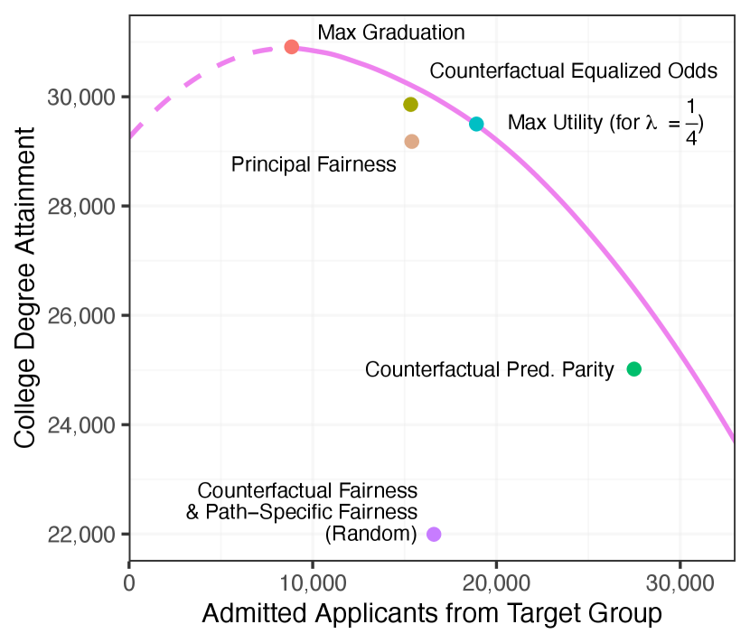
For the utility function in Eq. (6) with $\lambda=\tfrac{1}{4}$, we apply Theorem B.1 to compute utility-maximizing policies for each of the above causal definitions of fairness. We plot the results in Figure 2, where, for each policy, the horizontal axis shows the expected number of admitted applicants from the target race group, and the vertical axis shows the expected number of college graduates. Additionally, for the family of utilities $\mathcal{U}$ given by Eq. (6) for $\lambda\geq 0$, we depict the Pareto frontier by the solid purple curve, computed via Proposition 1.⁸⁸8For all the cases we consider, the optimal policies admit the maximum proportion of students allowed under the budget $b$ (i.e., $\operatorname{Pr}(D=1)=b$). To compute the Pareto frontier in Figure 2, it is sufficient—by Proposition 1 and Footnote 7—to sweep over (standardized) group-specific threshold policies relative to the utility $u_{0}(x)=\mathbb{E}[Y(1)|X=x]$. For reference, the dashed purple line corresponds to max-utility policies constrained to satisfy the level of diversity indicated on the $x$-axis, though these policies are not on the Pareto frontier, as they result in fewer college graduates and lower diversity than the policy that maximizes graduation alone (indicated by the “max graduation” point in Figure 2).

For each fairness definition, the depicted policies are strongly Pareto dominated, meaning that there is an alternative feasible policy favored by all decision makers with preferences in $\mathcal{U}$. In particular, for each definition of causal fairness, there is an alternative feasible policy in which one simultaneously achieves more student-body diversity and more college graduates. In some instances, the efficiency gap is quite stark. Utility-maximizing policies constrained to satisfy either counterfactual fairness or path-specific fairness require one to admit each applicant independently with fixed probability $b$ (where $b$ is the budget), regardless of academic preparedness or group membership.⁹⁹9For path-specific fairness, we set $\Pi$ equal to the single path $A\rightarrow E\rightarrow T\rightarrow D$, and set $W=X$ in this example. These results show that constraining decision-making algorithms to satisfy popular definitions of causal fairness can have unintended consequences, and may even harm the very groups they were ostensibly designed to protect.

The patterns illustrated in Figure 2 and discussed above are not idiosyncracies of our particular example, but rather hold quite generally. Indeed, Theorem 1 shows that for almost every joint distribution of $X$, $Y(0)$, and $Y(1)$ such that $u(X)$ has a density, any decision policy satisfying counterfactual equalized odds or conditional principal fairness is Pareto dominated. Similarly, for almost every joint distribution of $X$ and $X_{\Pi,A,a}$, we show that policies satisfying path-specific fairness (including counterfactual fairness) are Pareto dominated. (NB: The analogous statement for counterfactual predictive parity is not true, which we address in Proposition 2.)

The notion of almost every distribution that we use here was formalized by Christensen (1972), Hunt et al. (1992), Anderson & Zame (2001), and others (cf. Ott & Yorke, 2005, for a review). Suppose, for a moment, that combinations of covariates and outcomes take values in a finite set of size $m$. Then the space of joint distributions on covariates and outcomes can be represented by the unit $(m-1)$-simplex: $\Delta^{m-1}=\{p\in\mathbb{R}^{m}\mid p_{i}\geq 0\ \text{and}\ \sum_{i=1}^{m}p_{i}=1\}$. Since $\Delta^{m-1}$ is a subset of an $(m-1)$-dimensional hyperplane in $\mathbb{R}^{m}$, it inherits the usual Lebesgue measure on $\mathbb{R}^{m-1}$. In this finite-dimensional setting, almost every distribution means a subset of distributions that has full Lebesgue measure on the simplex. Given a property that holds for almost every distribution in this sense, that property holds almost surely under any probability distribution on the space of distributions that is described by a density on the simplex. We use a generalization of this basic idea that extends to infinite-dimensional spaces, allowing us to consider distributions with arbitrary support. (See the Appendix for further details.)

To prove this result, we make relatively mild restrictions on the set of distributions and utilities we consider to exclude degenerate cases, as formalized by Definition 9 below.

In particular, $\mathcal{U}$-fineness ensures that the distribution of $u(X)$ has a density. In the absence of $\mathcal{U}$-fineness, corner cases can arise in which an especially large number of policies may be Pareto efficient, in particular when $u(X)$ has large atoms and $X$ can be used to predict the potential outcomes $Y(0)$ and $Y(1)$ even after conditioning on $u(X)$. See Prop. E.7 for details. Our example of college admissions, where $\mathcal{U}$ is defined by Eq. (6), is $\mathcal{U}$-fine.

The proof of Theorem 1 is given in the Appendix. At a high-level, the proof proceed in three steps, which we outline below using the example of counterfactual equalized odds. First, we show that for almost every fixed $\mathcal{U}$-fine joint distribution $\mu$ of $X$ and $Y(1)$ there is at most one policy $d^{*}(x)$ satisfying counterfactual equalized odds that is not strongly Pareto dominated. To see why, note that for any specific $y_{0}$, since counterfactual equalized odds requires that $D\mathchoice{\mathrel{\hbox to0.0pt{$\displaystyle\perp$\hss}\mkern 2.0mu{\displaystyle\perp}}}{\mathrel{\hbox to0.0pt{$\textstyle\perp$\hss}\mkern 2.0mu{\textstyle\perp}}}{\mathrel{\hbox to0.0pt{$\scriptstyle\perp$\hss}\mkern 2.0mu{\scriptstyle\perp}}}{\mathrel{\hbox to0.0pt{$\scriptscriptstyle\perp$\hss}\mkern 2.0mu{\scriptscriptstyle\perp}}}A\mid Y(1)=y_{0}$, setting the threshold for one group determines the thresholds for all the others; the budget constraint then can be used to fix the threshold for the original group. Second, we construct a “slice” around $\mu$ such that for any distribution $\nu$ in the slice, $d^{*}(x)$ is still the only policy that can potentially lie on the Pareto frontier while satisfying counterfactual equalized odds. We create the slice by strategically perturbing $\mu$ only where $Y(1)=y_{1}$, for some $y_{1}\neq y_{0}$. This perturbation moves mass from one side of the thresholds of $d^{*}(x)$ to the other, consequently breaking the balance requirement $D\mathchoice{\mathrel{\hbox to0.0pt{$\displaystyle\perp$\hss}\mkern 2.0mu{\displaystyle\perp}}}{\mathrel{\hbox to0.0pt{$\textstyle\perp$\hss}\mkern 2.0mu{\textstyle\perp}}}{\mathrel{\hbox to0.0pt{$\scriptstyle\perp$\hss}\mkern 2.0mu{\scriptstyle\perp}}}{\mathrel{\hbox to0.0pt{$\scriptscriptstyle\perp$\hss}\mkern 2.0mu{\scriptscriptstyle\perp}}}A\mid Y(1)=y_{1}$ for almost every $\nu$ in the slice. This phenomenon is similar to the problem of infra-marginality (Simoiu et al., 2017; Ayres, 2002), which likewise afflicts non-causal notions of fairness (Corbett-Davies et al., 2017; Corbett-Davies & Goel, 2018). Finally, we appeal to the notion of prevalence to stitch the slices together, showing that for almost every distribution, any policy satisfying counterfactual equalized odds is strongly Pareto dominated. Analogous versions of this general argument apply to the cases of conditional principal fairness and path-specific fairness.¹¹¹¹11This argument does not depend in an essential way on the definitions being causal. In Corollary E.5, we show an analogous result for the non-counterfactual version of equalized odds.

In some common settings, path-specific fairness with $W=X$ constrains decisions so severely that the only allowable policies are constant (i.e., $d(x_{1})=d(x_{2})$ for all $x_{1},x_{2}\in\mathcal{X}$). For instance, in our running example, path-specific fairness requires admitting all applicants with the same probability, irrespective of academic preparation or group membership. Thus, all applicants are admitted with probability $b$, where $b$ is the budget, under the optimal policy constrained to satisfy path-specific fairness.

To build intuition for this result, we sketch the argument for a finite covariate space $\mathcal{X}$. Given a policy $d$ that satisfies path-specific fairness, select $x^{*}\in\arg\max_{x\in\mathcal{X}}d(x)$.

By the definition of path-specific fairness, for any $a\in\mathcal{A}$,

That is, the probability of an individual with covariates $x^{*}$ receiving a positive decision must be the average probability of the individuals with covariates $x$ in group $a$ receiving a positive decision, weighted by the probability that an individual with covariates $x^{*}$ in the real world would have covariates $x$ counterfactually.

Next, we suppose that there exists an $a^{\prime}\in\mathcal{A}$ such that $\operatorname{Pr}(X_{\Pi,A,a^{\prime}}=x\mid X=x^{*})>0$ for all $x\in\alpha^{-1}(a^{\prime})$. In this case, because $d(x)\leq d(x^{*})$ for all $x\in\mathcal{X}$, Eq. (9) shows that in fact $d(x)=d(x^{*})$ for all $x\in\alpha^{-1}(a^{\prime})$.

Now, let $x^{\prime}$ be arbitrary. Again, by the definition of path-specific fairness, we have that

where we use in the third equality the fact $d(x)=d(x^{*})$ for all $x\in\alpha^{-1}(a^{\prime})$, and in the final equality the fact that $X_{\Pi,A,a^{\prime}}$ is supported on $\alpha^{-1}(a^{\prime})$.

Theorem 2 formalizes and extends this argument to more general settings, where $\operatorname{Pr}(X_{\Pi,A,a^{\prime}}=x\mid X=x^{*})$ is not necessarily positive for all $x\in\alpha^{-1}(a^{\prime})$. The proof of Theorem 2 is in the Appendix, along with extensions to continuous covariate spaces and a more complete characterization of $\Pi$-fair policies for finite $\mathcal{X}$.

The first condition of Theorem 2 holds for any reduced set of covariates $Z$ that is not causally affected by changes in $A$ (e.g., $Z$ is not a descendent of $A$). The second condition requires that among individuals with covariates $x$, a positive fraction have covariates $x^{\prime}$ in a counterfactual world in which they belonged to another group $a^{\prime}$. Because $\zeta(x)$ is the same in the real and counterfactual worlds—since $Z$ is unaffected by $A$, by the first condition—we only consider $x^{\prime}$ such that $\zeta(x^{\prime})=\zeta(x)$ in the second condition.

In our running example, the only non-race covariate is test score, which is downstream of race. Further, among students with a given test score, a positive fraction achieve any other test score in the counterfactual world in which their race is altered. As such, the empty set of reduced covariates—formally encoded by setting $\zeta$ to a constant function—satisfies the conditions of Theorem 2. The theorem then implies that under any $\Pi$-fair policy, every applicant is admitted with equal probability.

Even when decisions are not perfectly uniform lotteries, as in our admissions example, Theorem 2 suggests that enforcing $\Pi$-fairness can lead to unexpected outcomes. For instance, suppose we modify our admissions example to additionally include age as a covariate that is causally unconnected to race—as some past work has done. In that case, $\Pi$-fair policies would admit students based on their age alone, irrespective of test score or race. Although in some cases such restrictive policies might be desirable, this strong structural constraint implied by $\Pi$-fairness appears to be a largely unintended consequence of the mathematical formalism.

The conditions of Theorem 2 are relatively mild, but do not hold in every setting. Suppose that in our admissions example it were the case that $T_{\Pi,A,a_{0}}=T_{\Pi,A,a_{1}}+c$ for some constant $c$—that is, suppose the effect of intervening on race is a constant change to an applicant’s test score. Then the second condition of Theorem 2 would no longer hold for a constant $\zeta$. Indeed, any multiple-threshold policy in which $t_{a_{0}}=t_{a_{1}}+c$ would be $\Pi$-fair. In practice, though, such deterministic counterfactuals would seem to be the exception rather than the rule. For example, it seems reasonable to expect that test scores would depend on race in complex ways that induce considerable heterogeneity.

Lastly, we note that $W\neq X$ in some variants of path-specific fairness (e.g., Zhang & Bareinboim, 2018; Nabi & Shpitser, 2018), in which case Theorem 2 does not apply. Although, in that case, policies are typically still Pareto dominated in accordance with Theorem 1.

We conclude our analysis by investigating counterfactual predictive parity, the least demanding of the causal notions of fairness we have considered, requiring only that $Y(1)\mathchoice{\mathrel{\hbox to0.0pt{$\displaystyle\perp$\hss}\mkern 2.0mu{\displaystyle\perp}}}{\mathrel{\hbox to0.0pt{$\textstyle\perp$\hss}\mkern 2.0mu{\textstyle\perp}}}{\mathrel{\hbox to0.0pt{$\scriptstyle\perp$\hss}\mkern 2.0mu{\scriptstyle\perp}}}{\mathrel{\hbox to0.0pt{$\scriptscriptstyle\perp$\hss}\mkern 2.0mu{\scriptscriptstyle\perp}}}A\mid D=0$. As such, it is in general possible to have a policy on the Pareto frontier that satisfies this condition. However, in Proposition 2, we show that this cannot happen in some common cases, including our example of college admissions.

In that setting, when the target group has lower average graduation rates—a pattern that often motivates efforts to actively increase diversity—decision policies constrained to satisfy counterfactual predictive parity are Pareto dominated. The proof of the proposition is in the Appendix.

References

- Anderson & Zame (2001) Anderson, R. M. and Zame, W. R. Genericity with infinitely many parameters. Advances in Theoretical Economics, 1(1):1–62, 2001.
- Ayres (2002) Ayres, I. Outcome tests of racial disparities in police practices. Justice Research and Policy, 4(1-2):131–142, 2002.
- Benji (2020) Benji. The sum of an uncountable number of positive numbers. Mathematics Stack Exchange, 2020. URL https://math.stackexchange.com/q/20661. (version: 2020-05-29).
- Berk et al. (2021) Berk, R., Heidari, H., Jabbari, S., Kearns, M., and Roth, A. Fairness in criminal justice risk assessments: The state of the art. Sociological Methods & Research, 50(1):3–44, 2021.
- Bertrand & Mullainathan (2004) Bertrand, M. and Mullainathan, S. Are Emily and Greg more employable than Lakisha and Jamal? A field experiment on labor market discrimination. American Economic Review, 94(4):991–1013, 2004.
- Billingsley (1995) Billingsley, P. Probability and Measure. Wiley Series in Probability and Mathematical Statistics. John Wiley & Sons, Inc., New York, third edition, 1995. ISBN 0-471-00710-2. A Wiley-Interscience Publication.
- Brozius (2019) Brozius, H. Conditional expectation - . Mathematics Stack Exchange, 2019. URL https://math.stackexchange.com/q/3247577. (Version: 2019-06-01).
- Cai et al. (2020) Cai, W., Gaebler, J., Garg, N., and Goel, S. Fair allocation through selective information acquisition. In Proceedings of the AAAI/ACM Conference on AI, Ethics, and Society, pp. 22–28, 2020.
- Carey & Wu (2022) Carey, A. N. and Wu, X. The causal fairness field guide: Perspectives from social and formal sciences. Frontiers in Big Data, 5, 2022.
- Chiappa (2019) Chiappa, S. Path-specific counterfactual fairness. In Proceedings of the AAAI Conference on Artificial Intelligence, volume 33, pp. 7801–7808, 2019.
- Chohlas-Wood et al. (2021a) Chohlas-Wood, A., Coots, M., Brunskill, E., and Goel, S. Learning to be fair: A consequentialist approach to equitable decision-making. arXiv preprint arXiv:2109.08792, 2021a.
- Chohlas-Wood et al. (2021b) Chohlas-Wood, A., Nudell, J., Yao, K., Lin, Z., Nyarko, J., and Goel, S. Blind justice: Algorithmically masking race in charging decisions. In Proceedings of the 2021 AAAI/ACM Conference on AI, Ethics, and Society, pp. 35–45, 2021b.
- Chouldechova (2017) Chouldechova, A. Fair prediction with disparate impact: A study of bias in recidivism prediction instruments. Big data, 5(2):153–163, 2017.
- Chouldechova & Roth (2020) Chouldechova, A. and Roth, A. A snapshot of the frontiers of fairness in machine learning. Communications of the ACM, 63(5):82–89, 2020.
- Christensen (1972) Christensen, J. P. R. On sets of Haar measure zero in Abelian Polish groups. Israel Journal of Mathematics, 13(3-4):255–260, 1972.
- Cleary (1968) Cleary, T. A. Test bias: Prediction of grades of Negro and white students in integrated colleges. Journal of Educational Measurement, 5(2):115–124, 1968.
- Corbett-Davies & Goel (2018) Corbett-Davies, S. and Goel, S. The measure and mismeasure of fairness: A critical review of fair machine learning. arXiv preprint arXiv:1808.00023, 2018.
- Corbett-Davies et al. (2017) Corbett-Davies, S., Pierson, E., Feller, A., Goel, S., and Huq, A. Algorithmic decision making and the cost of fairness. In Proceedings of the 23rd ACM SIGKDD International Conference on Knowledge Discovery and Data Mining, pp. 797–806, 2017.
- Coston et al. (2020) Coston, A., Mishler, A., Kennedy, E. H., and Chouldechova, A. Counterfactual risk assessments, evaluation, and fairness. In Proceedings of the 2020 Conference on Fairness, Accountability, and Transparency, pp. 582–593, 2020.
- Darlington (1971) Darlington, R. B. Another look at “cultural fairness”. Journal of Educational Measurement, 8(2):71–82, 1971.
- Dwork et al. (2012) Dwork, C., Hardt, M., Pitassi, T., Reingold, O., and Zemel, R. Fairness through awareness. In Proceedings of the 3rd Innovations in Theoretical Computer Science Conference, pp. 214–226, 2012.
- Gaebler et al. (2022) Gaebler, J., Cai, W., Basse, G., Shroff, R., Goel, S., and Hill, J. A causal framework for observational studies of discrimination. Statistics and Public Policy, 2022.
- Galhotra et al. (2022) Galhotra, S., Shanmugam, K., Sattigeri, P., and Varshney, K. R. Causal feature selection for algorithmic fairness. Proceedings of the 2022 International Conference on Management of Data (SIGMOD), 2022.
- Goel et al. (2017) Goel, S., Perelman, M., Shroff, R., and Sklansky, D. A. Combatting police discrimination in the age of big data. New Criminal Law Review: An International and Interdisciplinary Journal, 20(2):181–232, 2017.
- Goldin & Rouse (2000) Goldin, C. and Rouse, C. Orchestrating impartiality: The impact of “blind” auditions on female musicians. American Economic Review, 90(4):715–741, 2000.
- Greiner & Rubin (2011) Greiner, D. J. and Rubin, D. B. Causal effects of perceived immutable characteristics. Review of Economics and Statistics, 93(3):775–785, 2011.
- Grogger & Ridgeway (2006) Grogger, J. and Ridgeway, G. Testing for racial profiling in traffic stops from behind a veil of darkness. Journal of the American Statistical Association, 101(475):878–887, 2006.
- Hardt et al. (2016) Hardt, M., Price, E., and Srebro, N. Equality of opportunity in supervised learning. Advances in Neural Information Processing Systems, 29:3315–3323, 2016.
- Holland (1986) Holland, P. W. Statistics and causal inference. Journal of the American Statistical Association, 81(396):945–960, 1986.
- Hu & Kohler-Hausmann (2020) Hu, L. and Kohler-Hausmann, I. What’s sex got to do with machine learning? In Proceedings of the 2020 ACM Conference on Fairness, Accountability, and Transparency, 2020.
- Hunt et al. (1992) Hunt, B. R., Sauer, T., and Yorke, J. A. Prevalence: a translation-invariant “almost every” on infinite-dimensional spaces. Bulletin of the American Mathematical Society, 27(2):217–238, 1992.
- Imai & Jiang (2020) Imai, K. and Jiang, Z. Principal fairness for human and algorithmic decision-making. arXiv preprint arXiv:2005.10400, 2020.
- Imai et al. (2020) Imai, K., Jiang, Z., Greiner, J., Halen, R., and Shin, S. Experimental evaluation of algorithm-assisted human decision-making: Application to pretrial public safety assessment. arXiv preprint arXiv:2012.02845, 2020.
- Imbens & Rubin (2015) Imbens, G. W. and Rubin, D. B. Causal Inference in Statistics, Social, and Biomedical Sciences. Cambridge University Press, 2015.
- Kasy & Abebe (2021) Kasy, M. and Abebe, R. Fairness, equality, and power in algorithmic decision-making. In Proceedings of the 2021 ACM Conference on Fairness, Accountability, and Transparency, pp. 576–586, 2021.
- Kemeny & Snell (1976) Kemeny, J. G. and Snell, J. L. Finite Markov Chains. Undergraduate Texts in Mathematics. Springer-Verlag, New York-Heidelberg, 1976. Reprinting of the 1960 original.
- Kilbertus et al. (2017) Kilbertus, N., Rojas-Carulla, M., Parascandolo, G., Hardt, M., Janzing, D., and Schölkopf, B. Avoiding discrimination through causal reasoning. In Proceedings of the 31st International Conference on Neural Information Processing Systems, pp. 656–666, 2017.
- Kleinberg et al. (2017) Kleinberg, J., Mullainathan, S., and Raghavan, M. Inherent trade-offs in the fair determination of risk scores. In 8th Innovations in Theoretical Computer Science Conference (ITCS). Schloss Dagstuhl-Leibniz-Zentrum fuer Informatik, 2017.
- Kusner et al. (2017) Kusner, M., Loftus, J., Russell, C., and Silva, R. Counterfactual fairness. In Proceedings of the 31st International Conference on Neural Information Processing Systems, pp. 4069–4079, 2017.
- Liang et al. (2021) Liang, A., Lu, J., and Mu, X. Algorithmic design: Fairness versus accuracy. arXiv preprint arXiv:2112.09975, 2021.
- Liu et al. (2018) Liu, L. T., Dean, S., Rolf, E., Simchowitz, M., and Hardt, M. Delayed impact of fair machine learning. In International Conference on Machine Learning, pp. 3150–3158. PMLR, 2018.
- Loftus et al. (2018) Loftus, J. R., Russell, C., Kusner, M. J., and Silva, R. Causal reasoning for algorithmic fairness. arXiv preprint arXiv:1805.05859, 2018.
- Mhasawade & Chunara (2021) Mhasawade, V. and Chunara, R. Causal multi-level fairness. In Proceedings of the 2021 AAAI/ACM Conference on AI, Ethics, and Society, pp. 784–794, 2021.
- Mishler et al. (2021) Mishler, A., Kennedy, E. H., and Chouldechova, A. Fairness in risk assessment instruments: Post-processing to achieve counterfactual equalized odds. In Proceedings of the 2021 ACM Conference on Fairness, Accountability, and Transparency, pp. 386–400, 2021.
- Nabi & Shpitser (2018) Nabi, R. and Shpitser, I. Fair inference on outcomes. In Proceedings of the AAAI Conference on Artificial Intelligence, volume 32, 2018.
- Ott & Yorke (2005) Ott, W. and Yorke, J. Prevalence. Bulletin of the American Mathematical Society, 42(3):263–290, 2005.
- Page (2007) Page, S. E. Making the difference: Applying a logic of diversity. Academy of Management Perspectives, 21(4):6–20, 2007.
- Pearl (2001) Pearl, J. Direct and indirect effects. In Proceedings of the Seventeenth Conference on Uncertainty and Artificial Intelligence, 2001, pp. 411–420. Morgan Kaufman, 2001.
- Pearl (2009a) Pearl, J. Causal inference in statistics: An overview. Statistics surveys, 3:96–146, 2009a.
- Pearl (2009b) Pearl, J. Causality. Cambridge University Press, second edition, 2009b.
- Pierson et al. (2020) Pierson, E., Simoiu, C., Overgoor, J., Corbett-Davies, S., Jenson, D., Shoemaker, A., Ramachandran, V., Barghouty, P., Phillips, C., Shroff, R., and Goel, S. A large-scale analysis of racial disparities in police stops across the United States. Nature Human Behaviour, 4(7):736–745, 2020.
- Rao (2005) Rao, M. M. Conditional measures and applications, volume 271 of Pure and Applied Mathematics (Boca Raton). Chapman & Hall/CRC, Boca Raton, FL, second edition, 2005.
- Rudin (1987) Rudin, W. Real and Complex Analysis. McGraw-Hill Book Co., New York, third edition, 1987. ISBN 0-07-054234-1.
- Rudin (1991) Rudin, W. Functional Analysis. International Series in Pure and Applied Mathematics. McGraw-Hill, Inc., New York, second edition, 1991. ISBN 0-07-054236-8.
- Silva (2008) Silva, C. E. Invitation to Ergodic Theory, volume 42 of Student Mathematical Library. American Mathematical Society, Providence, RI, 2008.
- Simoiu et al. (2017) Simoiu, C., Corbett-Davies, S., and Goel, S. The problem of infra-marginality in outcome tests for discrimination. The Annals of Applied Statistics, 11(3):1193–1216, 2017.
- Steele (2019) Steele, R. Space of vector measures equipped with the total variation norm is complete. Mathematics Stack Exchange, 2019. URL https://math.stackexchange.com/q/3197508. (Version: 2019-04-22).
- Wang et al. (2019) Wang, Y., Sridhar, D., and Blei, D. M. Equal opportunity and affirmative action via counterfactual predictions. arXiv preprint arXiv:1905.10870, 2019.
- Williams (1983) Williams, T. S. Some issues in the standardized testing of minority students. Journal of Education, pp. 192–208, 1983.
- Woodworth et al. (2017) Woodworth, B., Gunasekar, S., Ohannessian, M. I., and Srebro, N. Learning non-discriminatory predictors. In Conference on Learning Theory, pp. 1920–1953. PMLR, 2017.
- Wu et al. (2019) Wu, Y., Zhang, L., Wu, X., and Tong, H. PC-fairness: A unified framework for measuring causality-based fairness. Advances in Neural Information Processing Systems, 32, 2019.
- Zafar et al. (2017a) Zafar, M. B., Valera, I., Gomez Rodriguez, M., and Gummadi, K. P. Fairness beyond disparate treatment & disparate impact: Learning classification without disparate mistreatment. In Proceedings of the 26th International Conference on World Wide Web, pp. 1171–1180, 2017a.
- Zafar et al. (2017b) Zafar, M. B., Valera, I., Rodriguez, M. G., Gummadi, K. P., and Weller, A. From parity to preference-based notions of fairness in classification. In Proceedings of the 31st International Conference on Neural Information Processing Systems, pp. 228–238, 2017b.
- Zhang & Bareinboim (2018) Zhang, J. and Bareinboim, E. Fairness in decision-making—the causal explanation formula. In Thirty-Second AAAI Conference on Artificial Intelligence, 2018.
- Zhang et al. (2017) Zhang, L., Wu, Y., and Wu, X. A causal framework for discovering and removing direct and indirect discrimination. In Proceedings of the 26th International Joint Conference on Artificial Intelligence, pp. 3929–3935, 2017.
Appendix A Path-specific Counterfactuals
Constructing policies which satisfy path-specific fairness requires computing path-specific counterfactual values of features. In Algorithm 1, we describe the formal construction of path-specific counterfactuals , for an arbitrary variable (or collection of variables) in the DAG. To generate a sample from the distribution of , we first sample values for the exogenous variables. Then, in the first loop, we traverse the DAG in topological order, setting to and iteratively computing values of the other nodes based on the structural equations in the usual fashion. In the second loop, we set to , and then iteratively compute values for each node. is computed using the structural equation at that node, with value for each of its parents that are connected to it along a path in , and the value for all its other parents. Finally, we set to .
Appendix B Constructing Causally Fair Policies
In order to construct causally fair policies, we prove that the optimization problem in Eq. (7) can be efficiently solved as a single linear program—in the case of counterfactual equalized odds, conditional principal fairness, counterfactual fairness, and path-specific fairness—or as a series of linear programs in the case of counterfactual predictive parity.
Theorem B.1.
Consider the optimization problem given in Eq. (7).
-
1.
If is the class of policies that satisfies counterfactual equalized odds or conditional principal fairness, and the distribution of is known and supported on a finite set of size , then a utility-maximizing policy constrained to lie in can be constructed via a linear program with variables and constraints.
2.
If is the class of policies that satisfies path-specific fairness (including counterfactual fairness), and the distribution of is known and supported on a finite set of size , then a utility-maximizing policy constrained to lie in can be constructed via a linear program with variables and constraints.
3.
Suppose is the class of policies that satisfies counterfactual predictive parity, that the distribution of is known and supported on a finite set of size , and that the optimization problem in Eq. (7) has a feasible solution. Further suppose is supported on points, and let be the unit -simplex. Then one can construct a set of linear programs , with each having variables and constraints, such that the solution to one of the LPs in is a utility-maximizing policy constrained to lie in .
Proof.
Let ; then, we seek decision variables , , corresponding to the probability of making a positive decision for individuals with covariate value . Therefore, we require that .
Letting denote the mass of at , note that the objective function equals and the budget constraint are both linear in the decision variables.
We now show that each of the causal fairness definitions can be enforced via linear constraints. We do so in three parts as listed in theorem.
Theorem B.1 Part 1
First, we consider counterfactual equalized odds. A decision policy satisfies counterfactual equalized odds when Since is binary, this condition is equivalent to the expression for all and such that . Expanding this expression and replacing by the corresponding decision variable , we obtain that
for each and each of the finitely many values such that . These constraints are linear in the by inspection.
Next, we consider conditional principal fairness. A decision policy satisfies conditional principal fairness when , where denotes a reduced set of the covariates . Again, since is binary, this condition is equivalent to the expression for all , , and satisfying . As above, expanding this expression and replacing by the corresponding decision variable yields linear constraints of the form
for each and each of the finitely many values of such that satisfies . Again, these constraints are linear by inspection.
Theorem B.1 Part 2
Suppose a decision policy satisfies path-specific fairness for a given collection of paths and a (possibly) reduced set of covariates meaning that for every , .
Recall from the definition of path-specific counterfactuals that , where . Since , , it follows that
An analogous calculation yields that . Equating these expressions gives
for each and each of the finitely many such that . Again, each of these constraints is linear by inspection.
Theorem B.1 Part 3
A decision policy satisfies counterfactual predictive parity if or equivalently, for all . We may rewrite this expression to obtain:
where .
Expanding the numerator on the left-hand side of the above equation yields
Similarly, expanding the denominator yields
for each of the finitely many . Therefore, counterfactual predictive parity corresponds to