Causal Effect of Functional Treatment
Abstract
Functional data often arise in the areas where the causal treatment effect is of interest. However, research concerning the effect of a functional variable on an outcome is typically restricted to exploring the association rather than the casual relationship. The generalized propensity score, often used to calibrate the selection bias, is not directly applicable to a functional treatment variable due to a lack of definition of probability density function for functional data. Based on the functional linear model for the average dose-response functional, we propose three estimators, namely, the functional stabilized weight estimator, the outcome regression estimator and the doubly robust estimator, each of which has its own merits. We study their theoretical properties, which are corroborated through extensive numerical experiments. A real data application on electroencephalography data and disease severity demonstrates the practical value of our methods.
Keywords: double robustness; functional data analysis; functional linear model; functional stabilized weight; treatment effect.
1 Introduction
In observational studies, a fundamental question is to investigate the causal effect of a treatment variable on an outcome. Traditionally, a large amount of works focus on a binary treatment variable (i.e., treatment versus control); see e.g., Rosenbaum and Rubin (1983); Hirano et al. (2003); Imai and Ratkovic (2014, 2015); Chan et al. (2016); Athey et al. (2018); Ding et al. (2019); Tan (2020); Guo et al. (2021). Recently, there is a growing interest in studying more complex treatment variables, e.g., categorical (Lopez and Gutman, 2017a, b; Li and Li, 2019) and continuous variables (Hirano and Imbens, 2004; Galvao and Wang, 2015; Kennedy et al., 2017; Fong et al., 2018; Kennedy, 2019; Ai et al., 2021; Bonvini and Kennedy, 2022).
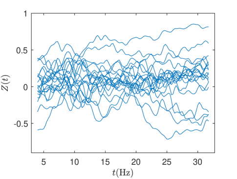
Our interest is to estimate the average dose-response functional (ADRF) of a functional treatment variable. Functional data, usually collected repeatedly over a continuous domain, arise in many fields such as astronomy, economics and biomedical sciences. Such data are essentially of infinite dimension and thus fundamentally different from scalar variables; see Wang et al. (2016) for a review on functional data analysis. Our setting is substantially distinct from those of the observational longitudinal studies (Robins, 2000; Robins et al., 2000; Moodie and Stephens, 2012; Imai and Ratkovic, 2015; Zhao et al., 2015; Kennedy, 2019), where the treatment variable takes binary values at each time point and the outcome variable also depends on time. In contrast, the functional treatment variable considered here is real-valued over a continuous domain (not limited to time but can be space, frequency, etc.) and the outcome variable is a scalar that does not vary with respect to (w.r.t.) that continuous domain. Real data applications of our setting can be found in the literature on the scalar-on-function regression; see Morris (2015) for a review. For example, we may be interested in the causal relationship between daily temperature and crop harvest (Wong et al., 2019), spectrometric data and fat content of certain types of food (Ferraty and Vieu, 2006), daily air pollution and mortality rate (Kong et al., 2016), etc. Our work is motivated by an electroencephalography (EEG) dataset (Ciarleglio et al., 2022), which was collected to investigate possible causation between the human neuronal activities and severity of the major depressive disorder. A random subsample of 20 frontal asymmetric curves measuring intensity of the human neuronal activities is shown in Figure 1.
In a nonrandomized observational study, it is impossible to identify the causal effect without imposing any assumption. In addition to basic assumptions like the stable unit treatment value assumption, consistency and positivity, a routinely used condition for identification is the unconfoundedness assumption (Rosenbaum and Rubin, 1983) i.e., the potential outcome is independent of the treatment given all the confounding covariates. For a continuous scalar treatment, under the unconfoundedness assumption, the generalized propensity score or the stabilized weight (Hirano and Imbens, 2004; Imai and van Dyk, 2004; Galvao and Wang, 2015; Kennedy et al., 2017; Ai et al., 2021; Bonvini and Kennedy, 2022) has been widely used to calibrate the selection bias, which relies upon the (conditional) density of the treatment variable. However, the probability density function of functional data generally does not exist (Delaigle and Hall, 2010). Therefore, in our context, neither of the generalized propensity score or stabilized weight is well defined, and thus the traditional methods are not directly applicable. To circumvent the problem, Zhang et al. (2021) proposed to approximate the functional treatment variable based on functional principal component analysis (FPCA) and defined a stabilized weight function by the (conditional) probability density of the PC scores to adjust the selection bias. However, their estimator is not well defined when the number of PCs tends to infinity and thus asymptotic consistency is not guaranteed.
Under the unconfoundedness assumption in the context of a functional treatment variable, we propose three estimators of the ADRF, including a functional stabilized weight (FSW) method, a partially linear outcome regression (OR) method and a doubly robust (DR) approach by combining the two. Specifically, the first estimator assumes a functional linear model for the ADRF and incorporates a new FSW. In contrast to Zhang et al. (2021), our FSW is well defined and guarantees the identification of the ADRF. By constructing a novel consistent nonparametric estimator of the FSW, we can estimate the ADRF by functional linear regression with the weighted outcome. Our second estimator assumes a more restrictive linear model taking the confounding variables into account. The model quantifies the ADRF by the expectation of the linear model with respect only to the confounding variables, which is computed through a backfitting algorithm. Further, by combining the first two estimators, we propose a new DR estimator, which is consistent if either of the first two estimators is consistent. In particular, it enjoys a fast convergence rate as the second estimator if the partially linear model is correctly specified; while it imposes less restrictive modelling assumptions as the first estimator, which is still consistent although has a slower convergence rate. Such double robustness is different from those in the literature on a continuous scalar treatment variable (see e.g., Kennedy et al., 2017; Bonvini and Kennedy, 2022), where the DR estimator is consistent if one of two models for the conditional outcome and the generalized propensity score is correctly specified. In our case, the functional linear model for the ADRF is required for the consistency of all the three estimators; and the FSW, serving the role of the generalized propensity score, is estimated nonparametrically.
The rest of the paper is organized as follows. We introduce the basic setup for identification of ADRF in Section 2, followed by development of our three estimators in Section 3. We investigate the convergence rates of the estimators in Section 4, and provide detailed cross-validation procedures for selecting tuning parameters in Section 5. The simulation and the real data analysis are presented in Sections 6 and 7, respectively. Section 8 concludes with discussion, and the supplementary material contains all the technical details.
2 Identification of Average Dose-Response Functional
We consider a functional treatment variable such that the observed treatment variable, denoted by , is a smooth real-valued random function defined on a compact interval , with . Let be the potential outcome given the treatment for , the Hilbert space of squared integrable functions on . For each individual, we only observe a random treatment and the corresponding outcome . We are interested in estimating the ADRF, , for any .
Unlike an observational longitudinal study (Robins, 2000; Robins et al., 2000; Moodie and Stephens, 2012; Imai and Ratkovic, 2015; Zhao et al., 2015; Kennedy, 2019), here we assume that the outcome variable does not depend on , where the interval is not limited to representing a time interval, but can also be a space, a domain of frequencies, etc. Instead of considering the association between and as in the traditional regression setting, here we investigate their causal relationship. We assume that the functional variable is fully or densely observed. Essentially, our methodology can be applied when is only sparsely observed as long as the trajectory of can be well reconstructed, while development of asymptotic properties in such cases would be much more challenging (Zhang and Wang, 2016).
A fundamental problem of causal inference is that we never observe simultaneously for all . This is a more severe issue in our context, compared to the traditional scalar treatment case, because is a functional variable valued in an infinite dimensional space. It is then impossible to identify from the observed data alone without any assumption. Let be the -dimensional observable confounding covariates that are related to both and . We impose the following assumptions in order to identify .
Assumption 1
-
(i)
Unconfoundedness: Given , is independent of for all , i.e., .
-
(ii)
Stable unit treatment value assumption: There is no interference among the units, i.e., each individual’s outcome depends only on their own level of treatment intensity.
-
(iii)
Consistency: a.s. if .
-
(iv)
Positivity: The conditional density satisfies a.s.
Assumption 1 is a natural extension of the classical identification assumption in the literature of scalar treatment effect (Rosenbaum and Rubin, 1983; Hirano and Imbens, 2004; Kennedy et al., 2017) to the context of a functional treatment variable. The positivity condition (iv) in Assumption 1 is different from that widely used for identifying the scalar treatment effect, where the generalized propensity score, defined by the probability density of the treatment variable conditional on the confounding covariates, is required to be positive. However, the probability and the conditional probability density functions of functional data, i.e., and , generally do not exist (Delaigle and Hall, 2010). To circumvent this problem, we impose the positivity condition for the conditional density , which is well defined.
Under Assumption 1, the ADRF can be identified from the observable variables in the following three ways,
| (2.1) |
Alternatively, we have
| (2.2) |
where is called the functional stabilized weight (FSW). Note that if were a scalar random variable, we have , where the right-hand side is the classical stabilized weight. Let denote the expectation w.r.t. . Noting that and , together with (2.1) and (2.2), we can also identify as
| (2.3) |
3 Models and Estimation Methods
For all the three methods, we make the following functional linear model assumption on the ADRF:
| (3.1) |
where is the scalar intercept, and is the slope function. Such model is widely used in the literature of scalar-on-function regression. Under such a model, the slope function becomes the quantity of primary interest convenient for the causal inference, because it measures the intensity of the functional treatment effect. For example, to compute the average treatment effect (ATE), , of two given , it suffices to compute .
3.1 Functional Stabilized Weight Estimator
Our functional stabilized weight (FSW) estimator does not rely on any model assumption other than (3.1). In particular, equation (2.2) suggests that we can estimate in (3.1) using the classical functional linear regression technique (e.g., Hall and Horowitz, 2007) with the response variable replaced by , provided an estimator of . To facilitate the development, suppose that an estimator of is available for now. Let be the covariance function of . Its eigenvalues and the corresponding orthonormal eigenfunctions are defined as follows,
| (3.2) |
where , also called the PC basis, is a complete basis of . According to the Karhunen–Loéve expansion, we have
| (3.3) |
where and .
With no ambiguity, let denote the linear operator such that , for a function . Combining (2.2), (3.1) and (3.3), we can write
where . It follows that , where . Noting that is an orthonormal complete basis of , we can write and , and combining with (3.2), we obtain for all that
The above argument suggests that we can estimate by with being a truncation parameter and , where the ’s and ’s are the eigenvalues and the eigenfunctions of the empirical covariance function , respectively, and is the empirical estimator of . Also, the estimator of is given by
with . We then define . Finally, the estimator of is given by .
It remains to estimate the FSW, . In particular, we need to estimate the weights at the sample points, , for . A naive approach would first estimate the densities and and then take the ratio, which, however, may lead to unstable estimates because an estimator of the denominator is difficult to derive and may be too close to zero. Also, approximating by its PC scores would not alleviate the challenge but pose additional difficulty in theoretical justification. To circumvent these problems, we treat as a whole and develop a robust nonparametric estimator. The idea of estimating the density ratio directly has also been exploited in Ai et al. (2021) for a scalar treatment variable. However, their method is not applicable to the functional treatment.
Specifically, when the treatment was a scalar, Ai et al. (2021) found that the moment equation
| (3.4) |
holds for any integrable functions and and it identifies . Denoting the support of by , they further estimated the function by maximizing a generalized empirical likelihood, subject to the restriction of the empirical counterpart of (3.4), where the spaces of integrable functions and are approximated by a growing number of basis functions; see Section 4 of Ai et al. (2021) for details. However, those restrictions are not applicable in our context where is a random function in . In particular, it is unclear whether (3.4) still identifies . Moreover, the space of functionals is generally nonseparable, which impedes a consistent approximation of using the basis expansion.
To overcome the challenge of estimating , we derive a novel expanding set of equations that can identify from functional data and avoid approximating a general functional . Specifically, instead of estimating the function , we estimate its projection for every fixed , and find that
| (3.5) |
holds for any integrable function . In particular, the following proposition shows that (3.5) indeed identifies the function for every fixed .
Proposition 3.1.
For any fixed ,
holds for all integrable functions if and only if a.s.
The proof is given in Supplement A. This result indicates that is fully characterized by (3.5), and thus we can use it to define our estimator. Since (3.5) is defined for a fixed and we need to estimate at all sample points , we consider the leave-one-out index set to estimate at each . Specifically, for a given sample point , the right-hand side of (3.5) can be estimated by its empirical version , and we propose to estimate the left-hand side of (3.5) by the Nadaraya–Watson estimator for a functional covariate (see e.g., Ferraty and Vieu, 2006),
where denotes a semi-metric in , is a bandwidth and is a kernel function quantifying the proximity of and . Commonly used choices for include the norm and the projection metric , where denotes a projection operation to a subspace of . The projection metric may yield better asymptotic properties; see Section 4 for more details, and see Section 5 on how to choose and .
As it is not possible to solve (3.5) for an infinite number of ’s from a given finite sample, we use a growing number of basis functions to approximate any suitable function . Specifically, let be a set of known basis functions, which may serve as a finite dimensional sieve approximation to the original function space of all integrable functions. We define our estimator of , for , as the solution to the equations,
| (3.6) |
which asymptotically identifies as and . However in practice, a finite number of equations as in (3.6) are not able to identify a unique solution. Indeed, for any strictly increasing and concave function , replacing by would satisfy (3.6), where is the first derivative of and is a -dimensional vector maximizing the strictly concave function defined as
| (3.7) |
This can be verified by noting that the gradient corresponds to (3.6) with replaced by . Therefore, for a given strictly increasing and concave function together with defined above, we define our estimator of as , which also induces the estimator by replacing by .
To gain more insight on the function , we investigate the generalized empirical likelihood interpretation of our estimator. As shown in Supplement B, the estimator defined by (3.7) is the dual solution to the following local generalized empirical likelihood maximization problem. For each , ,
| (3.8) |
where is a distance measure between and 1 for . The function is continuously differentiable satisfying and , where is the inverse function of , the first derivative of . The sample moment restriction stabilizes our weight estimator.
Our estimator is the desired weight closest to the baseline uniform weight 1 locally around a small neighbourhood of each , subject to the finite sample version of the moment restriction in Proposition 3.1. The uniform weight can be considered as a baseline because when and are unconditionally independent for all (i.e., a randomized trial without confoundedness), the functional stabilized weights should be uniformly equal to 1. Different choices of correspond to different distance measures. For example, if we take , then is the information entropy and the weights correspond to the exponential tilting (Imbens et al., 1998). Other choices include with , the empirical likelihood (Owen, 1988), and with , yielding the implied weights of the continuous updating of the generalized method of moments (Hansen et al., 1996). We suggest to choose which guarantees a positive weight estimator .
3.2 Outcome Regression Estimator and Doubly Robust Estimator
To estimate the ADRF based on the outcome regression (OR) identification method in (2.1), an estimator of is required. Thus, based on the functional linear model in (3.1), we further assume the following partially linear model,
| (3.9) |
where and are the same as those in (3.1), is the slope coefficient for and is the error variable with and uniformly for all and . Without loss of generality, we assume that ; otherwise the non-zero mean can be absorbed into .
Recalling from (2.1), we can see that (3.9) implies (3.1). Indeed, model (3.9) imposes a stronger structure than model (3.1). For example, the linear part can be replaced by any nonparametric function of , which still implies model (3.1). However, model (3.9) gives a simpler estimator of with a faster convergence rate and a better interpretability of the effects of the treatment and the confounding variables on the outcome.
It remains to estimate the unknown parameters and in (3.9), for which the backfitting algorithm (Buja et al., 1989) can be adapted to our context. In the first step, we set to be zero and apply the same method as in Section 3.1 to regress on , which gives the initial estimators of and in (3.9). Specifically, we estimate initially by with , where the ’s and ’s are the same as those in Section 3.1, while with . We then define . Finally, the initial estimator of is defined as .
In the second step, we use the traditional least square method to regress the residual on , for . Specifically, we estimate by , where is an matrix with the -th entry being , the -th element of , and
Subsequently, we can repeat the first step with replaced by to update the estimators of and . This procedure is iterated until the outcome regression (OR) estimators of , and , denoted by , and , are stabilized.
The OR estimator is easy to implement but requires strong parametric assumptions, while the FSW estimator requires less modelling assumptions but subject to a slow convergence rate. It is thus of interest to develop an estimator by combining these two that possesses more attractive properties.
Note that (2.3) satisfies the so-called doubly robust (DR) property: for two generic functions and , it holds that
| (3.10) |
if either or but not necessarily both are satisfied; see Supplement C for the derivation.
Under model (3.1), (3.10) equals . To estimate and , it suffices to conduct the functional linear regression as in Section 3.1 to regress an estimator of on . Specifically, we estimate by the OR estimator, , and by . We define the DR estimator of as , where with . Here, is defined as
where
Also, the DR estimator of is defined as .
Provided that model (3.1) is correctly specified, according to the DR property (3.10), the DR estimator is consistent if either or is consistent. The consistency of mainly depends on correct specification of the partially linear model (3.9), while the consistency of , as a nonparametric estimator, relies on less restrictive (but technical) assumptions; see Section 4 for details.
4 Asymptotic Properties
We investigate asymptotic convergence rates of our proposed three estimators. Recall that our main model is as in (3.1). Although the estimators of are based on the estimators of , they are essentially empirical mean estimators, which can achieve the convergence rate; see Shin (2009). Thus, our primary focus is to derive the convergence rates of our estimators of , which, depending on the smoothness of and , are slower than those in the finite dimensional settings.
Recall that denotes the support of , and let be the support of . To derive the convergence rate of , we first provide the uniform convergence rate of the estimator of the FSW over and , which requires the following conditions.
Condition A
-
(A1)
The set is compact. For all and , is strictly bounded away from zero and infinity.
-
(A2)
For all , and a constant such that , where is the inverse function of .
-
(A3)
The eigenvalues of are bounded away from zero and infinity uniformly in and . There exists a sequence of constants satisfying .
-
(A4)
There exists a continuously differentiable function , for , such that for all , is strictly bounded away from zero and infinity. There exists such that is bounded.
-
(A5)
The kernel is bounded, Lipschitz and supported on with .
-
(A6)
For and , there exists such that for all and all , all and all , and are bounded.
-
(A7)
Let be the Kolmogorov -entropy of , i.e., , where is the minimal number of open balls in of radius (with the semi-metric ) covering . It satisfies for some , and for large enough.
Condition (A1) requires that is compactly supported, which can be relaxed by restricting the tail behaviour of the distribution of at the sacrifice of more tedious technical arguments. The boundedness of in Condition (A1) (or some equivalent condition) is also commonly required in the literature (Kennedy et al., 2017; Ai et al., 2021; D’Amour et al., 2021). This condition can be relaxed if other smoothness assumptions are made on the potential outcome distribution (Ma and Wang, 2020). Condition (A2) essentially assumes that the convergence rate of the sieve approximation for is polynomial. This can be satisfied, for example, with if is discrete, and with if has continuous components and is a power series, where is the degree of smoothness of w.r.t. the continuous components in for any fixed . Further, Condition (A3) ensures that the sieve approximation conditional on a functional variable is not degenerate. Similar conditions are routinely assumed in the literature of sieve approximation (Newey, 1997). Conditions (A4) to (A6) are standard in functional nonparametric regression (Ferraty and Vieu, 2006; Ferraty et al., 2010). In particular, the function in Condition (A4), also referred to as the small ball probability, has been studied extensively in the literature (Li and Shao, 2001; Ferraty and Vieu, 2006); Condition (A5) requires that is compactly supported, which is not satisfied for the Gaussian kernel but convenient for technical arguments; the variable in Condition (A6) serves as the role of the response variable in the traditional regression setting. Condition (A7) is less standard: it regularizes the support by controlling its Kolmogorov entropy, which is used to establish the uniform convergence rate on . This condition is satisfied, for example, if is a compact set, is a projection metric and ; see Ferraty et al. (2010) for other examples.
Theorem 4.1 provides the sup-norm convergence rate of over the support of and . The proof is given in Supplement D. The term and the term can be viewed as the convergence rates of the bias and standard deviation, respectively.
To provide the convergence rate of , we recall that under model (3.1). Let be the residual variable. Let and be two constants and the ’s be some generic positive constants.
Condition B
-
(B1)
The variable has a finite fourth moment, i.e., .
- (B2)
-
(B3)
The coefficient satisfies , for all .
Condition (B1) makes a mild restriction on the moment of . Condition (B2) imposes regularity conditions on the random process , which, in particular, requires that the differences of the adjacent eigenvalues do not decay too fast. Condition (B3) assumes an upper bound for the decay rate of , the coefficients of projected on . The latter two conditions are adopted from Hall and Horowitz (2007) for technical purposes.
Theorem 4.2.
The proof of Theorem 4.2 is given in Supplement E. The convergence rate of in Theorem 4.2 can be quite slow mainly because of the small ball probability function . In the case of Gaussian process endowed with a metric, has an exponential decay rate of (Li and Shao, 2001), which leads to a non-infinitesimal rate of . However, can be much larger by choosing a proper semi-metric (Ferraty and Vieu, 2006; Ling and Vieu, 2018) so that the final convergence rate of reaches a polynomial decay of . Another way to improve the convergence rate is to impose additional structure assumptions. For example, if we assume that the slope function can be fully characterized by a finite number of PC basis functions, or the random process essentially lies on a finite dimensional space (not necessarily Euclidean; see Lin and Yao, 2021), then the truncation parameter does not need to tend to infinity and the convergence rate of can be much faster. Without such assumptions, estimating in an infinite dimensional space with a nonparametric estimator of leads to a cumbersome convergence rate.
The OR estimator relies on FPCA and the partially linear model (3.9). Additional conditions are needed to derive the convergence rate of .
Condition C
-
(C1)
The covariate has finite fourth moment, i.e., . For and , .
-
(C2)
Let and . For , , and is positive definite with .
Conditions (C1) and (C2) adopted from Shin (2009) make mild assumptions on the covariate to ensure -consistency of the estimated coefficient .
Theorem 4.3.
Because is theoretically equivalent to the least square estimator proposed by Shin (2009) provided that each component estimator is unique (Buja et al., 1989), the theorem above is a direct result from Theorem 3.2 in Shin (2009) and thus its proof is omitted. The convergence rate of is the same as that of the estimated slope function in the traditional functional linear regression (see Hall and Horowitz, 2007), i.e., such rate remains unchanged despite of the additional estimation of . Compared with Theorem 4.2, the convergence rate here is much faster. Specifically, the part of the convergence rate , which is the convergence rate of , is replaced by a faster one , because the nonparametric estimator is not used.
According to the DR property (3.10), the estimator inherits advantages from and , depending on which conditions are satisfied. Specifically, if model (3.1) is correctly specified, has the same convergence rate as given that the conditions in Theorem 4.2 are satisfied. If the stronger model assumption (3.9) holds, then enjoys the faster convergence rate as , provided that Condition C is satisfied.
5 Selection of Tuning Parameters
For the FSW estimator, our methodology requires a kernel function with a metric , basis functions and tuning parameters , and . Using a compactly supported kernel would make the denominator of the first term in (3.7) too small for some and destabilize the maximization of in (3.7). Therefore, we suggest using the Gaussian kernel, , with the semi-metric being the norm. To develop an estimating strategy for that is applicable for a generic dataset, we standardize the ’s and use a unified set of choices for . Letting , , we transform the ’s,
so that they have support on . Let be the -th component of and be the -th standard Legendre polynomial on . If were given, we define and , for , and . We restrict the range of such that is a positive integer, and orthonormalize the resulting matrix .
We suggest to select and jointly by an -fold cross validation (CV). Specifically, we randomly split the dataset into parts, . Let denote the remaining sample with excluded. We define the CV loss,
where is the estimated PC score, , and are obtained by applying the method in Section 3.1 to . We choose the one from a given candidate set of such that is minimized.
For the OR estimator, we need to select the truncation parameter , which can be chosen by an -fold CV similar to the above derivation. Specifically, we consider
where , and are obtained by applying the method in Section 3.2 to . From a given candidate set of , we choose the one that minimizes .
Similarly, for the DR estimator, we still need to select the truncation parameter . This can be done by minimizing the CV loss,
where denotes the number of elements in , , , are obtained by applying the methods in Section 3.2 to .
6 Simulation Study
As the ADRF is parametrized by a functional linear model, , we mainly focus on the performances of the estimators of , which measures the intensity of the functional treatment effect. In addition to the methods of functional stabilized weight (FSW), outcome regression (OR) and double robustness (DR) developed in Section 3, we also consider the method using the nonparametric principal component weight (PCW) proposed by Zhang et al. (2021), which assumes the same functional linear model for the ADRF, as well as the Naive method directly using the functional linear regression of on .
We choose the number of PCs used in estimating the PCW so as to explain 95% of the variance of following Zhang et al. (2021), and take for FSW with . For a fair comparison, we use such truncation parameter in estimating for all other methods.
| Model | FSW | OR | DR | PCW | Naive | |
|---|---|---|---|---|---|---|
| (i) | 20.44 (32.44) | 19.39 (26.33) | 20.34 (29.14) | 37.24 (47.63) | 47.32 (33.41) | |
| 8.66 (11.91) | 7.73 (14.05) | 7.94 (14.08) | 23.58 (34.93) | 33.56 (16.27) | ||
| (ii) | 62.32 (68.12) | 79.71 (124.73) | 64.26 (100.92) | 69.14 (169.68) | 83.96 (131.40) | |
| 37.71 (42.06) | 39.23 (54.55) | 34.15 (49.04) | 35.62 (48.69) | 43.02 (57.89) | ||
| (iii) | 39.97 (39.36) | 43.99 (68.86) | 46.68 (72.61) | 96.56 (81.09) | 148.51 (69.76) | |
| 21.34 (13.11) | 13.94 (14.82) | 14.86 (17.36) | 66.68 (68.84) | 118.98 (27.22) | ||
| (iv) | 26.16 (27.40) | 58.16 (45.99) | 61.16 (54.35) | 114.26 (55.43) | 156.95 (51.66) | |
| 18.27 (17.56) | 48.42 (30.19) | 49.88 (35.27) | 91.86 (30.02) | 139.97 (32.99) |
We consider the sample sizes and 500. For , we generate the functional treatment , for , by , where , , , , , with the ’s being the independent standard normal variables, and for . For the slope function , we define . The ’s and are the same as those in Zhang et al. (2021). We consider four models for the covariate and the outcome variable :
-
(i)
and ,
-
(ii)
and ,
-
(iii)
and ,
-
(iv)
and ,
where and are generated independently. The PC scores of affect covariate linearly in models (i) and (ii) and nonlinearly in models (iii) and (iv), and covariate affects the outcome variable linearly in models (i) and (iii) and nonlinearly in models (ii) and (iv). The functional linear model (3.1) for the ADRF is correctly specified for all four models, while the partially linear model (3.9) is only correctly specified for models (i) and (iii). Due to the confounding effect of , the Naive method ignoring is expected to be biased. For each combination of model and sample size, we replicate 200 simulations and evaluate the results by the integrated squared error (ISE) of the slope function, , where denotes the estimator produced by the FSW, OR, DR, PCW and Naive methods, respectively.
Table 1 summarizes the mean and the standard deviation of the ISEs for all configurations. Our proposed estimators FSW, OR and DR show consistency with sample size increases, and outperform PCW and Naive almost in all the cases. In particular, our three estimators are close to each other and are better than those of PCW and Naive under models (i) and (iii), where covariate affects the outcome variable linearly. In the cases where the partially linear model (3.9) is misspecified, FSW and DR, followed closely by PCW, outperform OR under model (ii); FSW performs the best, followed by OR and DR, which still outperform PCW and Naive significantly under model (iv). Our results suggest that, in the case where the partially linear model is unlikely to hold, FSW or DR is preferred over OR. The performance of PCW is better than Naive but inferior to our methods under all models.
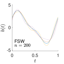
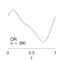
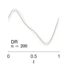
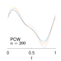
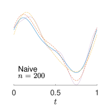
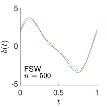
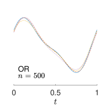
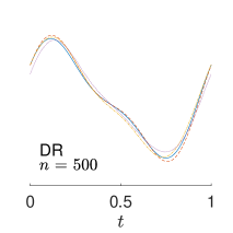
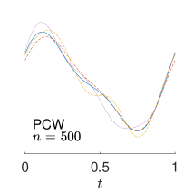
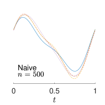
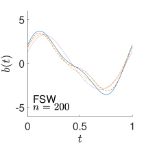
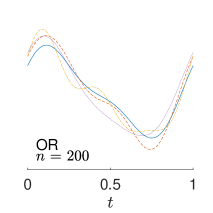
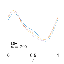
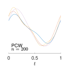
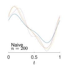
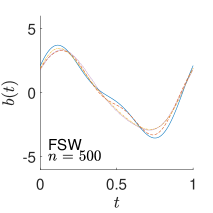
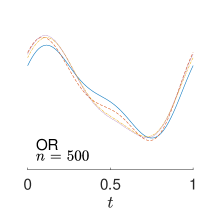
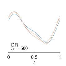
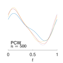
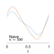
To give visualization of representative estimated slope functions, we show the so-called quartile curves of the samples corresponding to the first, second and third quartile values of 200 ISEs in Figure 2 for model (i). It can be seen that the estimated curves using all the methods except Naive are close to the truth, and those produced by PCW and Naive tend to be more variable than others. Figure 3 corresponds to the results under model (iv), i.e., a more challenging model structure. The differences among the estimators are more significant: FSW performs the best, followed by OR and DR, while PCW and Naive are more biased and variable than the first three.
7 Real Data Analysis
We illustrate estimation of the ADRF using the five methods, FSW, OR, DR, PCW and Naive, on the electroencephalography (EEG) dataset from Ciarleglio et al. (2022). The EEG is a relatively low-cost tool to measure human neuronal activities. The measurements are taken from multiple electrodes placed on scalps of subjects, and they are then processed and transformed to produce current source density curves on the frequency domain that provide information of the intensity of neuronal activities. In particular, the frontal asymmetry curves, considered as potential biomarkers for major depressive disorder, are treated as the functional treatment variable , for Hz. The outcome variable is defined as , where is the quick inventory of depressive symptomatology (QIDS) score measuring severity of depressive symptomatology. A larger value of indicates more severe depressive disorder. We are interested in investigating the causal effect of the intensity of neuronal activities represented by the frontal asymmetry curves on the severity of major depressive disorder. Potential confounding covariates include age , sex ( for female and for male) and Edinburgh Handedness Inventory score (ranging from to corresponding to completely left to right handedness). Individuals with missing are removed, which results in a sample of size 85 males and 151 females. The means (standard deviations) of , and are 2.73 (0.72), 35.97 (13.07) and 72.69 (48.76), respectively. For comparison of the estimated ADRF using different methods, the confounding variables are centralized.
As in Section 6, we use the number of PCs explaining 95% of the variance of (equal to for this dataset) in estimating PCW. We minimize with to choose the truncation parameter used in estimating the slope function for all methods as well as tuning parameters and used in FSW. As a result, explaining about 80% of the variance of is chosen to estimate the slope function.
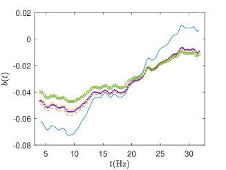
The left panel of Figure 4 shows the estimated slope functions. All the estimated slope functions have the same increasing trend over frequencies, while they have negative effect on the outcome variable for low frequencies. In other words, subjects with higher frontal asymmetry values on the low frequency domain tend to be healthier. This is consistent with the observations in Ciarleglio et al. (2022), where the authors found a negative association between the frontal asymmetry curves and the major depressive disorder status, using their functional regression model. More specifically, in the left panel of Figure 4, the estimated slope functions of FSW is the steepest and shows the largest effect in the low frequency domain. In contrast, the estimated slope function of Naive has overall smallest absolute values; the other three curves are quite close to each other.
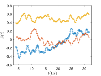
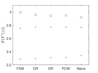
To illustrate visually the above negative effect found from the estimated slope function, we compute the estimated ADRF of three curves, which correspond to the smallest, median and largest average frontal asymmetry values over low frequencies 4 to 15 Hz. The middle panel of Figure 4 exhibits the selected curves and the right panel shows the corresponding estimated using all methods, which are around 2.9, 2.8 and 2.3 for the three curves, respectively.
8 Discussion
In the case of a functional treatment variable, we propose three estimators of the ADRF, namely, the FSW estimator, the OR estimator and the DR estimator, based on the functional linear model for the ADRF. The consistency of the FSW estimator relies on the functional linear model of by developing a nonparametric estimator of the weight; while the OR estimator requires a more restrictive linear model for in terms of . The DR estimator is consistent if either of the first two estimators is consistent. Asymptotic convergence rates are provided, and numerical results demonstrate great advantages of our methods.
It is of interest to construct the confidence band for the slope function to better quantify the ADRF or ATE, which, however, is difficult even in the simpler context of functional linear regression. As shown in Cardot et al. (2007), it is impossible for an estimator of the slope function to converge in distribution to a nondegenerate random element under the norm topology. For the OR estimator, it is possible to adapt the method proposed by Imaizumi and Kato (2019) to our context to construct an approximate confidence band. For the other two estimators, construction of the confidence band is challenging due to the less restrictive modelling assumption and the nonparametric estimator of the FSW, which warrants further investigation.
References
- Ai et al. (2021) Ai, C., O. Linton, K. Motegi, and Z. Zhang (2021). A unified framework for efficient estimation of general treatment models. Quantitative Economics 12(3), 779–816.
- Athey et al. (2018) Athey, S., G. W. Imbens, and S. Wager (2018). Approximate residual balancing: debiased inference of average treatment effects in high dimensions. Journal of the Royal Statistical Society: Series B (Statistical Methodology) 80(4), 597–623.
- Bonvini and Kennedy (2022) Bonvini, M. and E. H. Kennedy (2022). Fast convergence rates for dose-response estimation. arXiv preprint arXiv:2207.11825.
- Buja et al. (1989) Buja, A., T. Hastie, and R. Tibshirani (1989). Linear smoothers and additive models. The Annals of Statistics, 453–510.
- Cardot et al. (2007) Cardot, H., A. Mas, and P. Sarda (2007). Clt in functional linear regression models. Probability Theory and Related Fields 138(3), 325–361.
- Chan et al. (2016) Chan, K. C. G., S. C. P. Yam, and Z. Zhang (2016). Globally efficient non-parametric inference of average treatment effects by empirical balancing calibration weighting. Journal of the Royal Statistical Society: Series B (Statistical Methodology) 78(3), 673–700.
- Ciarleglio et al. (2022) Ciarleglio, A., E. Petkova, and O. Harel (2022). Elucidating age and sex-dependent association between frontal eeg asymmetry and depression: An application of multiple imputation in functional regression. Journal of the American Statistical Association 117(537), 12–26.
- Delaigle and Hall (2010) Delaigle, A. and P. Hall (2010). Defining probability density for a distribution of random functions. The Annals of Statistics 38(2), 1171–1193.
- Ding et al. (2019) Ding, P., A. Feller, and L. Miratrix (2019). Decomposing treatment effect variation. Journal of the American Statistical Association 114(525), 304–317.
- D’Amour et al. (2021) D’Amour, A., P. Ding, A. Feller, L. Lei, and J. Sekhon (2021). Overlap in observational studies with high-dimensional covariates. Journal of Econometrics 221(2), 644–654.
- Ferraty et al. (2010) Ferraty, F., A. Laksaci, A. Tadj, and P. Vieu (2010). Rate of uniform consistency for nonparametric estimates with functional variables. Journal of Statistical planning and inference 140(2), 335–352.
- Ferraty and Vieu (2006) Ferraty, F. and P. Vieu (2006). Nonparametric functional data analysis: theory and practice, Volume 76. Springer.
- Fong et al. (2018) Fong, C., C. Hazlett, and K. Imai (2018). Covariate balancing propensity score for a continuous treatment: Application to the efficacy of political advertisements. The Annals of Applied Statistics 12, 156–177.
- Galvao and Wang (2015) Galvao, A. F. and L. Wang (2015). Uniformly semiparametric efficient estimation of treatment effects with a continuous treatment. Journal of the American Statistical Association 110(512), 1528–1542.
- Guo et al. (2021) Guo, W., X.-H. Zhou, and S. Ma (2021). Estimation of optimal individualized treatment rules using a covariate-specific treatment effect curve with high-dimensional covariates. Journal of the American Statistical Association 116(533), 309–321.
- Hall and Horowitz (2007) Hall, P. and J. L. Horowitz (2007). Methodology and convergence rates for functional linear regression. The Annals of Statistics 35(1), 70–91.
- Hansen et al. (1996) Hansen, L. P., J. Heaton, and A. Yaron (1996). Finite-sample properties of some alternative gmm estimators. Journal of Business & Economic Statistics 14(3), 262–280.
- Hirano and Imbens (2004) Hirano, K. and G. W. Imbens (2004). The propensity score with continuous treatments. Applied Bayesian Modeling and Causal Inference from Incomplete-data Perspectives 226164, 73–84.
- Hirano et al. (2003) Hirano, K., G. W. Imbens, and G. Ridder (2003). Efficient estimation of average treatment effects using the estimated propensity score. Econometrica 71(4), 1161–1189.
- Imai and Ratkovic (2014) Imai, K. and M. Ratkovic (2014). Covariate balancing propensity score. Journal of the Royal Statistical Society: Series B (Statistical Methodology) 76(1), 243–263.
- Imai and Ratkovic (2015) Imai, K. and M. Ratkovic (2015). Robust estimation of inverse probability weights for marginal structural models. Journal of the American Statistical Association 110(511), 1013–1023.
- Imai and van Dyk (2004) Imai, K. and D. A. van Dyk (2004). Causal inference with general treatment regimes: Generalizing the propensity score. Journal of the American Statistical Association 99, 854–866.
- Imaizumi and Kato (2019) Imaizumi, M. and K. Kato (2019). A simple method to construct confidence bands in functional linear regression. Statistica Sinica 29(4), 2055–2081.
- Imbens et al. (1998) Imbens, G. W., R. H. Spady, and P. Johnson (1998). Information theoretic approaches to inference in moment condition models. Econometrica 66(2), 333.
- Kennedy (2019) Kennedy, E. H. (2019). Nonparametric causal effects based on incremental propensity score interventions. Journal of the American Statistical Association 114(526), 645–656.
- Kennedy et al. (2017) Kennedy, E. H., Z. Ma, M. D. McHugh, and D. S. Small (2017). Non-parametric methods for doubly robust estimation of continuous treatment effects. Journal of the Royal Statistical Society: Series B (Statistical Methodology) 79(4), 1229–1245.
- Kong et al. (2016) Kong, D., K. Xue, F. Yao, and H. H. Zhang (2016). Partially functional linear regression in high dimensions. Biometrika 103(1), 147–159.
- Li and Li (2019) Li, F. and F. Li (2019). Propensity score weighting for causal inference with multiple treatments. The Annals of Applied Statistics 13(4), 2389–2415.
- Li and Shao (2001) Li, W. V. and Q.-M. Shao (2001). Gaussian processes: inequalities, small ball probabilities and applications. Handbook of Statistics 19, 533–597.
- Lin and Yao (2021) Lin, Z. and F. Yao (2021). Functional regression on the manifold with contamination. Biometrika 108(1), 167–181.
- Ling and Vieu (2018) Ling, N. and P. Vieu (2018). Nonparametric modelling for functional data: selected survey and tracks for future. Statistics 52(4), 934–949.
- Lopez and Gutman (2017a) Lopez, M. J. and R. Gutman (2017a). Estimating the average treatment effects of nutritional label use using subclassification with regression adjustment. Statistical methods in medical research 26(2), 839–864.
- Lopez and Gutman (2017b) Lopez, M. J. and R. Gutman (2017b). Estimation of causal effects with multiple treatments: a review and new ideas. Statistical Science, 432–454.
- Ma and Wang (2020) Ma, X. and J. Wang (2020). Robust inference using inverse probability weighting. Journal of the American Statistical Association 115(532), 1851–1860.
- Moodie and Stephens (2012) Moodie, E. E. and D. A. Stephens (2012). Estimation of dose–response functions for longitudinal data using the generalised propensity score. Statistical methods in medical research 21(2), 149–166.
- Morris (2015) Morris, J. S. (2015). Functional regression. Annual Review of Statistics and Its Application 2, 321–359.
- Newey (1997) Newey, W. K. (1997). Convergence rates and asymptotic normality for series estimators. Journal of Econometrics 79(1), 147–168.
- Owen (1988) Owen, A. B. (1988). Empirical likelihood ratio confidence intervals for a single functional. Biometrika 75(2), 237–249.
- Robins (2000) Robins, J. M. (2000). Marginal structural models versus structural nested models as tools for causal inference. In Statistical models in epidemiology, the environment, and clinical trials, pp. 95–133. Springer.
- Robins et al. (2000) Robins, J. M., M. A. Hernan, and B. Brumback (2000). Marginal structural models and causal inference in epidemiology. Epidemiology 11(5), 550–560.
- Rosenbaum and Rubin (1983) Rosenbaum, P. R. and D. B. Rubin (1983). The central role of the propensity score in observational studies for causal effects. Biometrika 70, 45–55.
- Shin (2009) Shin, H. (2009). Partial functional linear regression. Journal of Statistical Planning and Inference 139(10), 3405–3418.
- Tan (2020) Tan, Z. (2020). Model-assisted inference for treatment effects using regularized calibrated estimation with high-dimensional data. The Annals of Statistics 48(2), 811–837.
- Wang et al. (2016) Wang, J.-L., J.-M. Chiou, and H.-G. Müller (2016). Functional data analysis. Annual Review of Statistics and its Application 3, 257–295.
- Wong et al. (2019) Wong, R. K., Y. Li, and Z. Zhu (2019). Partially linear functional additive models for multivariate functional data. Journal of the American Statistical Association 114(525), 406–418.
- Zhang and Wang (2016) Zhang, X. and J.-L. Wang (2016). From sparse to dense functional data and beyond. The Annals of Statistics 44(5), 2281–2321.
- Zhang et al. (2021) Zhang, X., W. Xue, and Q. Wang (2021). Covariate balancing functional propensity score for functional treatments in cross-sectional observational studies. Computational Statistics & Data Analysis.
- Zhao et al. (2015) Zhao, Y.-Q., D. Zeng, E. B. Laber, and M. R. Kosorok (2015). New statistical learning methods for estimating optimal dynamic treatment regimes. Journal of the American Statistical Association 110(510), 583–598.