Causal Identification of Sufficient, Contrastive and Complete Feature Sets
in Image Classification

Recent progress in artificial intelligence and the ever increasing deployment of AI systems has highlighted the need to understand better why some decisions are made by such systems. For example, one may need to know why a classifier decides that an MRI scan showed evidence of a tumor (Blake et al. 2023). Answering such questions is the province of causality. A causal explanation for an image classification is a special case of explanations in actual causality (Halpern 2019) and identifies a minimal set of pixels which, by themselves, are sufficient to re-create the original decision (Chockler and Halpern 2024).

Logic-based approaches provide formal guarantees for explanations, but their framework assumes that the model is given explicitly as a function. Their formal abductive explanations, or prime implicants (PI), are defined as sets of features such that, if they take the given values, always lead to the same decision (Shih, Choi, and Darwiche 2018). Logic-based methods can also compute contrastive explanations, that is, those features which, if altered, change the original decision. These abductive and contrastive explanations require a model to be monotonic or linear to be effectively computable (Marques-Silva et al. 2021), and therefore are not suitable for image classifiers.

In this paper, we show that causal explanations enjoy all the formal properties of logic-based explanations, while not putting any restrictions on the model and being efficiently computable for black-box image classifiers. We prove equivalence between abductive explanations and causal explanations and introduce a variation of causal explanations equivalent to contrastive explanations. Furthermore, we augment the actual causality framework with the model’s confidence in the classification, introducing $\delta$-confident explanations, and use these to produce more fine-grained results. We also introduce a causal version of the completeness property for explanations, following (Srinivas and Fleuret 2019). The differences between explanations of the classification of the same image reveal important information about the decision process of the model. In particular, we call the the difference between a complete explanation and a sufficient one adjustment pixels.

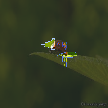
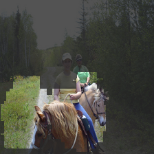
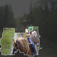
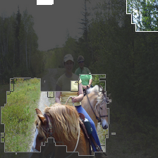
We examine the relationship between contrastive and adjustment pixel sets by examining the semantic distance between the original classification and the classifications of these pixel sets, as illustrated in Figure 1. Our approach allows us to formally subdivide an image into its sufficient pixels, contrastive pixels, and adjustment pixels. We prove complexity results for our definitions, giving a justification to efficient approximation algorithms.

Our algorithms are based on rex (Chockler et al. 2024). In Section 4 we introduce black-box approximation algorithms to compute contrastive, complete, and $\delta$-confident causal explanations for image classifiers. Our algorithms do not require any knowledge of the model, no access to the model internals, nor do they require any specific properties of the model. We implemented our algorithms and present experimental results on three state-of-the-art models and three standard benchmark datasets.

We use the word ‘explanation’ for the remainder of the paper as a convenience. We do not intend, nor seek to imply, that causal explanations are more or less interpretable than other form of explanation. Instead, we are interested in the formal partitioning of pixels in an image into different functional sets. These functional sets reveal important information about the inner workings of the model.

Due to the lack of space, some theoretical and evaluation results are deferred to the supplementary material.

There are many different definitions of explanation in the literature, some are saliency-based (Selvaraju et al. 2017), some are gradient-based (Srinivas and Fleuret 2019), Shapley-based (Lundberg and Lee 2017b) or train locally interpretable models (Ribeiro, Singh, and Guestrin 2016). Logic-based explanations are rather different in having a mathematically precise definition of explanation. Causal explanations, as defined in (Chockler and Halpern 2024) (and their approximations computed by rex (Chockler et al. 2024)), have much more in common with the rigorous definitions of logic-based explanations.

In this section we prove equivalences between definitions and properties satisfied by causal explanations. We start with formalization of logic-based explanations in the actual causality framework. For a given classification problem as defined in Section 2.3, we define a depth $2$ causal model $M$ as follows. The set of endogenous input variables is the set of features $\mathcal{F}$, with each variable $i\in\mathcal{F}$ having a domain $D_{i}$. The output of the classifier is the output variable $O$ of the model, with the domain $K$. An instance $(v,c)$ corresponds to a context $\vec{u}$ for $M$ that assigns to $\mathcal{F}$ the values defined by $v$, and the output is $c$. The set $\mathcal{K}$ of contexts is defined as the feature space $\mathbb{F}=D_{1}\times D_{2}\dots\times D_{m}$. As the classifier is not constant, there exist two inputs $v$ and $v^{\prime}$ such that $(M,v)\models O=c$, $(M,v^{\prime})\models O=c^{\prime}$, and $c\neq c^{\prime}$. It is easy to see that $M$ is a depth-$2$ causal model with all input variables being causally independent.

We use rex (Chockler et al. 2024) as a basis for computing the definitions provided in this paper. rex uses an approximation of causal responsibility to rank features. Responsibility is a quantitative measure of causality and, roughly speaking, measures the amount of causal influence on the classification (Chockler and Halpern 2004). Algorithm 1 details the greedy algorithm for approximation of $\delta$-sufficient-contrastive explanations, that is, explanations which are both sufficient and contrastive. Unfortunately, the precise computation of contrastive explanations is intractable, as follows from the intractability of actual causes in depth-$2$ causal models with independent inputs (Chockler et al. 2024).

We use a responsibility map created by rex (Algorithm 1, 4). A full description of rex can be found in Chockler et al. (2024).  rex approximates the causal responsibility of pixels in an image $I$ by performing an initial partition of $I$. Intuitively, a part of $I$ has the highest causal responsibility if it, by itself, is sufficient for the classification. A part of $I$ is lower in causal responsibility if it is not sufficient by itself, but it is sufficient together with several other parts. A part is completely irrelevant if it is neither. rex starts from large parts and then refines the important parts iteratively.

We use the resulting responsibility map to rank pixels by their responsibility for the desired classification. We use $2$ different sets of contexts, $\mathcal{K}^{+}$ and $\mathcal{K}^{-}$ (Algorithm 1, 5) to discover explanations. $\mathcal{K}^{+}$ is created by inserting pixels into an image created from the baseline occlusion value, as dictated by their approximate causal responsibility. In the case of a typical ImageNet model, which accepts an input tensor $224\times 224$, the total size of $\mathcal{K}^{+}$ is $50176$. In order to calculate the contrast of this, we also consider the opposite: the context $\mathcal{K}^{-}$, which replaces pixels from the original image with the baseline value, in accordance with their ranking by responsibility. The procedure is similar to the one used for insertion/deletion curves (Petsiuk, Das, and Saenko 2018). $\mathcal{K}^{+}$ ($\mathcal{K}^{-}$) is the set of contexts of all images produced by inserting (occluding) pixels, based on their pixel ranks, over a baseline value. In our experiments, we use the same baseline value for both $\mathcal{K}^{+}$ and $\mathcal{K}^{-}$. Our algorithm computes explanations which are both sufficient and contrastive.

Algorithm 2 details the procedure for extracting the adjustment pixels, given an image and a $\delta$-sufficient-contrastive explanation. In practice, the equality of 8 is difficult to achieve. Our implementation allows for a user-provided degree of precision. In our experiments, we set this to $4$ decimal places.

In this section, we present an analysis of various models and datasets viewed through the lens of contrast and completeness. To the best of our knowledge, there are no other tools that compute sufficient, contrastive and complete explanations for image classifiers. As shown in Section 3.2, these causal explanations have the same formal properties as logic-based explanations, but are also efficiently computable. Our algorithms have been included in the publicly available XAI tool rex ¹¹1https://github.com/ReX-XAI/ReX. rex was used with default parameters for all experiments, in particular, the random seed is $0$, baseline value $0$, and the number of iterations was $20$.

To the best of our knowledge, no-one has previously investigated the relationship of original classifications to contrastive explanations. Due to the hierarchical nature of the ImageNet dataset—it forms a tree—we can calculate the shortest path between the original classification and its contrastive class. We do the same with the completeness requirements, isolating the adjustment pixels, classifying them and calculating the shortest path to the original classification. For reasons of space, we include only a representative selection of results here. Complete results may be found in the supplementary material.

We examine $3$ models, all from TorchVision: a ResNet50, a MobileNet and Swin_t. All models were used with their default preprocessing procedures as provided by TorchVision. We also used $3$ different datasets, ImageNet-1K validation (approximately $4000$ images) (Russakovsky et al. 2015), PascalVoc20212 (Everingham et al. 2012) and a dataset of ‘complex’ images, ECSSD (Shi et al. 2016). We chose these datasets due to their being publicly available and well-studied. On a NVidia A100 GPU running Ubuntu LTS 22.04 we found that runtime varied greatly depending on the model under test. The ResNet50 and MobileNet were both very quick, taking approximately $6$ seconds per image. The Swin_t model was slower, taking approximately $16$ seconds per image. Our implementation makes extensive use of batched inference for efficiency, so models which do not accept batches will likely be slower.

Figure 4 shows the relative sizes of sufficient, contrastive and adjustment pixel sets for the $3$ different models on ImageNet. These are $\delta$-explanations where $\delta=1$. See supplementary material for other models and settings of $\delta$ . In general, ResNet50 requires the fewest pixels for both sufficiency and contrast, and also has very low adjustment pixel size. MobileNet and Swin_t appear to be much more similar in their behavior, though Swin_t has slightly greater contrastive requirements in general.

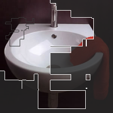
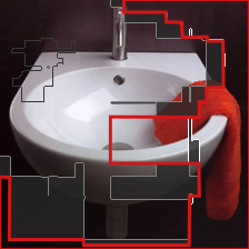
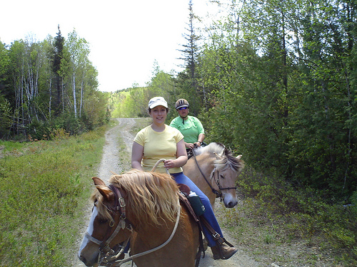
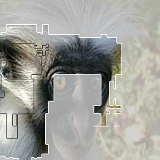
Figure 6 shows the shortest path between the original classification and its contrast class, according to the ImageNet hierarchy. In general, across all models, the distance between the two classes is not great, given that the maximum distance is $24$. This is not always the case, however: Figure 3(a) shows an example of a (mis-)classification where the contrast classification is ‘moped’. The adjustment pixels are classified as ‘picket fence’. It is worth noting that the initial confidence was already low on this image. At the other extreme Figure 6 reveals a few cases where the distance between the original classification and its contrast was very small. Manual inspection reveals that these cases represent refinements inside a larger class. Figure 5, for example, reveals the ResNet50 model required the highlighted pixels to refine the classification to colobus monkey. Without them, the classification is still monkey, but a different subclass – guenon.

We have demonstrated the concordances between logic-based and causal explanations. We have also introduced definitions for causal contrastive explanations and causal complete explanations. We have created algorithms for approximating these definitions and incorporated them into the tool rex. We have computed contrastive and complete explanations on $3$ different datasets with $3$ different models. We find that different models have different sufficiency, contrastive and adjustment requirements. Finally, we have examined the relationship between the original, contrastive and adjustment pixel predictions.

References

- Bach et al. (2015) Bach, S.; Binder, A.; Montavon, G.; Klauschen, F.; Müller, K.-R.; and Samek, W. 2015. On Pixel-wise Explanations for Non-linear Classifier Decisions by Layer-wise Relevance Propagation. PLOS One, 10(7).
- Beckers (2021) Beckers, S. 2021. Causal sufficiency and actual causation. Journal of Philosophical Logic, 50: 1341–1374.
- Blake et al. (2023) Blake, N.; Chockler, H.; Kelly, D. A.; Pena, S. C.; and Chanchal, A. 2023. MRxaI: Black-Box Explainability for Image Classifiers in a Medical Setting. arXiv preprint arXiv:2311.14471.
- Chockler and Halpern (2004) Chockler, H.; and Halpern, J. Y. 2004. Responsibility and Blame: A Structural-Model Approach. J. Artif. Intell. Res., 22: 93–115.
- Chockler and Halpern (2024) Chockler, H.; and Halpern, J. Y. 2024. Explaining Image Classifiers. In Proceedings of the 21st International Conference on Principles of Knowledge Representation and Reasoning, KR.
- Chockler, Kelly, and Kroening (2025) Chockler, H.; Kelly, D. A.; and Kroening, D. 2025. Multiple Different Explanations for Image Classifiers. In ECAI European Conference on Artificial Intelligence.
- Chockler et al. (2024) Chockler, H.; Kelly, D. A.; Kroening, D.; and Sun, Y. 2024. Causal Explanations for Image Classifiers. arXiv preprint arXiv:2411.08875.
- Everingham et al. (2012) Everingham, M.; Van Gool, L.; Williams, C. K. I.; Winn, J.; and Zisserman, A. 2012. The PASCAL Visual Object Classes Challenge 2012 (VOC2012) Results. http://www.pascal-network.org/challenges/VOC/voc2012/workshop/index.html.
- Glymour and Wimberly (2007) Glymour, C.; and Wimberly, F. 2007. Actual causes and thought experiments. In Campbell, J.; O’Rourke, M.; and Silverstein, H., eds., Causation and Explanation, 43–67. Cambridge, MA: MIT Press.
- Griffin, Holub, and Perona (2022) Griffin, G.; Holub, A.; and Perona, P. 2022. Caltech 256.
- Hall (2007) Hall, N. 2007. Structural equations and causation. Philosophical Studies, 132: 109–136.
- Halpern (2019) Halpern, J. Y. 2019. Actual Causality. The MIT Press.
- Halpern and Pearl (2005) Halpern, J. Y.; and Pearl, J. 2005. Causes and explanations: a structural-model approach. Part I: causes. British Journal for Philosophy of Science, 56(4): 843–887.
- Hitchcock (2001) Hitchcock, C. 2001. The intransitivity of causation revealed in equations and graphs. Journal of Philosophy, XCVIII(6): 273–299.
- Hitchcock (2007) Hitchcock, C. 2007. Prevention, preemption, and the principle of sufficient reason. Philosophical Review, 116: 495–532.
- Ignatiev et al. (2020) Ignatiev, A.; Narodytska, N.; Asher, N.; and Marques-Silva, J. 2020. On Relating ’Why?’ and ’Why Not?’ Explanations. CoRR, abs/2012.11067.
- Ignatiev, Narodytska, and Marques-Silva (2019) Ignatiev, A.; Narodytska, N.; and Marques-Silva, J. 2019. Abduction-based explanations for Machine Learning models. In Proceedings of the Thirty-Third AAAI Conference on Artificial Intelligence and Thirty-First Innovative Applications of Artificial Intelligence Conference and Ninth AAAI Symposium on Educational Advances in Artificial Intelligence, AAAI’19/IAAI’19/EAAI’19. AAAI Press. ISBN 978-1-57735-809-1.
- Izza et al. (2024) Izza, Y.; Ignatiev, A.; Stuckey, P. J.; and Marques-Silva, J. 2024. Delivering Inflated Explanations. Proceedings of the AAAI Conference on Artificial Intelligence, 38(11): 12744–12753.
- Kelly, Chanchal, and Blake (2025) Kelly, D. A.; Chanchal, A.; and Blake, N. 2025. I Am Big, You Are Little; I Am Right, You Are Wrong. In IEEE/CVF International Conference on Computer Vision, ICCV. IEEE.
- Kindermans et al. (2022) Kindermans, P.-J.; Hooker, S.; Adebayo, J.; Alber, M.; Schütt, K. T.; Dähne, S.; Erhan, D.; and Kim, B. 2022. The (Un)reliability of Saliency Methods, 267–280. Berlin, Heidelberg: Springer-Verlag. ISBN 978-3-030-28953-9.
- Lundberg and Lee (2017a) Lundberg, S. M.; and Lee, S.-I. 2017a. A Unified Approach to Interpreting Model Predictions. In Advances in Neural Information Processing Systems (NeurIPS), volume 30, 4765–4774.
- Lundberg and Lee (2017b) Lundberg, S. M.; and Lee, S.-I. 2017b. A Unified Approach to Interpreting Model Predictions. In Guyon, I.; Luxburg, U. V.; Bengio, S.; Wallach, H.; Fergus, R.; Vishwanathan, S.; and Garnett, R., eds., Advances in Neural Information Processing Systems, volume 30. Curran Associates, Inc.
- Marques-Silva et al. (2021) Marques-Silva, J.; Gerspacher, T.; Cooper, M. C.; Ignatiev, A.; and Narodytska, N. 2021. Explanations for Monotonic Classifiers. In Meila, M.; and Zhang, T., eds., Proceedings of the 38th International Conference on Machine Learning, volume 139 of Proceedings of Machine Learning Research, 7469–7479. PMLR.
- Miller (2019) Miller, T. 2019. Explanation in artificial intelligence: Insights from the social sciences. Artificial Intelligence, 267: 1–38.
- Papadimitriou and Yannakakis (1982) Papadimitriou, C. H.; and Yannakakis, M. 1982. The complexity of facets (and some facets of complexity). JCSS, 28(2): 244–259.
- Petsiuk, Das, and Saenko (2018) Petsiuk, V.; Das, A.; and Saenko, K. 2018. RISE: Randomized Input Sampling for Explanation of Black-box Models. In British Machine Vision Conference (BMVC). BMVA Press.
- Ribeiro, Singh, and Guestrin (2016) Ribeiro, M. T.; Singh, S.; and Guestrin, C. 2016. “Why Should I Trust You?” Explaining the Predictions of Any Classifier. In Knowledge Discovery and Data Mining (KDD), 1135–1144. ACM.
- Russakovsky et al. (2015) Russakovsky, O.; Deng, J.; Su, H.; Krause, J.; Satheesh, S.; Ma, S.; Huang, Z.; Karpathy, A.; Khosla, A.; Bernstein, M.; Berg, A. C.; and Fei-Fei, L. 2015. ImageNet Large Scale Visual Recognition Challenge. International Journal of Computer Vision (IJCV), 115(3): 211–252.
- Selvaraju et al. (2017) Selvaraju, R. R.; Cogswell, M.; Das, A.; Vedantam, R.; Parikh, D.; and Batra, D. 2017. Grad-CAM: Visual Explanations from Deep Networks via Gradient-based Localization. In International Conference on Computer Vision (ICCV), 618–626. IEEE.
- Shi et al. (2016) Shi, J.; Yan, Q.; Xu, L.; and Jia, J. 2016. Hierarchical Image Saliency Detection on Extended CSSD. IEEE Transactions on Pattern Analysis and Machine Intelligence, 38(4): 717–729.
- Shih, Choi, and Darwiche (2018) Shih, A.; Choi, A.; and Darwiche, A. 2018. A symbolic approach to explaining Bayesian network classifiers. In Proceedings of the 27th International Joint Conference on Artificial Intelligence, IJCAI’18, 5103–5111. AAAI Press. ISBN 9780999241127.
- Shrotri et al. (2022) Shrotri, A. A.; Narodytska, N.; Ignatiev, A.; Meel, K. S.; Marques-Silva, J.; and Vardi, M. Y. 2022. Constraint-Driven Explanations for Black-Box ML Models. Proceedings of the AAAI Conference on Artificial Intelligence, 36(8): 8304–8314.
- Srinivas and Fleuret (2019) Srinivas, S.; and Fleuret, F. 2019. Full-gradient representation for neural network visualization. In Proceedings of the 33rd International Conference on Neural Information Processing Systems. Red Hook, NY, USA: Curran Associates Inc.
- Weslake (2015) Weslake, B. 2015. A partial theory of actual causation. British Journal for the Philosophy of Science, To appear.
- Woodward (2003) Woodward, J. 2003. Making Things Happen: A Theory of Causal Explanation. Oxford, U.K.: Oxford University Press.
Appendix A Code and Data
Our algorithms have been included in the open source XAI tool rex. rex is available at https://github.com/ReX-XAI/ReX. Complete data and analysis code can be found at the following anonymous link https://figshare.com/s/7d822f952abcbe54ca93.
Appendix B Proofs
All definition references are to the main paper, unless explicitly stated otherwise.
Lemma 5.
For image classifiers, causal explanations (Definition 3) are abductive (Definition 5).
Proof.
For an instance , a set of variables and their values as defined by satisfy Definition 5 iff they satisfy EXIC1 in Definition 3. Moreover, is subset-minimal in iff it satisfies EXIC2 in Definition 3. Note that EXIC3 does not have an equivalent clause in the definition of abductive explanations, hence the other direction does not necessarily hold. ∎
Lemma 6.
Contrastive explanations (Definition 6) are equivalent to actual causes (Definition 1) in the same setting.
Recall that the framework of logic-based explanations translates to causal models of depth with all input variables being independent. An instance in Definition 6 exists iff for a context defined by , (AC1), where is the restriction of to the variables in . In this type of causal models, in AC2 is empty, hence Definition 6 holds for iff AC2 holds. Finally, is minimal iff AC3 holds. ∎
Lemma 7.
A contrastive explanation always exists.
Complete replacement of the pixels in an image is a contrastive explanation if no smaller subset is a contrastive explanation. ∎
This introduces a small complexity in the practical computation of contrastive explanations. It requires that the chosen baseline value does not that the same classification as an image , otherwise the baseline value does not introduce a contrastive element. rex checks for this problem automatically.
The following result follows from Lemma 6 and DP-completeness of actual causes in depth- causal models with independent inputs (Chockler et al. 2024). The class DP consists of those languages for which there exist a language in NP and a language in co-NP such that (Papadimitriou and Yannakakis 1982).
Lemma 8.
Given an input image, the decision problem of a contrastive explanation is DP-complete.
Proof follows Chockler, Kelly, and Kroening (2025) ∎
Appendix C Experimental Results
Figure 7 shows the results across all datasets and models with . In general, all models follow a fairly similar pattern. It is interesting to note that MobileNet requires more pixels in general for a causal explanation, but also the lowest number of pixels for adjustment. This suggests that, for MobileNet at least, the contrastive explanation encodes nearly all of its completeness into the contrastive explanation.
Figure 8 shows the length of the shortest path between the original classification and the adjustment pixels.
Appendix D Different
Figure 9 shows results for all datasets when the -confident explanation threshold is . If minimality is taken as a quality indicatory, this setting of sees a general deterioration of quality. The adjustment pixels sets are larger in general across all models and datasets. This suggests that this is a payoff between contrast and completeness: forcing the contrast explanation to have a higher confidence reduces the size of the adjustment pixel set, whereas a lower leads to a smaller contrast explanation and larger adjustment set. Users should bear this in mind when decided what aspect of a model’s behavior they wish to explore.
Figure 11 shows the distance in the ImageNet hierarchy across datasets and models, given a for contrastive explanations, i.e. the contrastive explanation must contain at least of the original confidence.
Appendix E Caltech-256
Figure 12 shows a small study on different classes from Caltech-256 (Griffin, Holub, and Perona 2022). These are, in general, simple images compared to ImageNet. The general pattern seen in Figure 7 does not change.
Figure 13 shows the contrast and adjustment distance in the ImageNet hierarchy on a small study of different classes from Caltech-256. This follows a similar pattern to Figure 6 in the main paper.