Causal Inference from Small High-dimensional Datasets
Abstract
Many methods have been proposed to estimate treatment effects with observational data. Often, the choice of the method considers the application’s characteristics, such as type of treatment and outcome, confounding effect, and the complexity of the data. These methods implicitly assume that the sample size is large enough to train such models, especially the neural network-based estimators. What if this is not the case? In this work, we propose Causal-Batle, a methodology to estimate treatment effects in small high-dimensional datasets in the presence of another high-dimensional dataset in the same feature space. We adopt an approach that brings transfer learning techniques into causal inference. Our experiments show that such an approach helps to bring stability to neural network-based methods and improve the treatment effect estimates in small high-dimensional datasets. The code for our method and all our experiments is available at github.com/causal-batle.
1 Introduction
Causal inference has received a lot of attention in the past few years. Being a trendy topic has its perks: it pushes the edge of methods, brings light to important discussions, incentives researchers to adopt best practices to make their methods reproducible, and creates new benchmarks. At the same time, some might be tired of reading ‘yet, another treatment effect estimator’. While it is true there is an abundance of treatment effect estimators; each method might be suitable for a different type of application: continuous versus binary treatments, single treatment versus multiple treatments, missing confounders versus causal sufficiency, low-dimensional datasets versus high-dimensional datasets, and the list goes on. Yet, in this work, we will propose another treatment effect estimator.
To illustrate our approach, consider a Computational Biology (CB) application: CB applications often have very detailed information from each patient, such as SNPs, genes, mutations, and parental information, but only a few patients. Hence, small high-dimensional datasets. The main bottleneck to collecting more samples is the high costs of finding new patients, plus the event’s rarity. In pharmacogenomics, for instance, some applications aim to explore the side effects of drugs adopted on certain pediatric cancer treatments. Collecting information about these patients is quite challenging for several reasons: first, it requires the families’ commitment in a very stressful and delicate time of their lives; second, it is a rare disease; finally, it requires a common effort between hospitals and doctors to refer the patients. While there are methods to estimate binary treatment effects [4, 6, 18, 19], and methods to estimate treatment effects with high-dimensional datasets [7], there is a lack of methods to estimate treatment effects in small high-dimensional datasets, such as the case of several computational biology applications.
In the Machine Learning (ML) community, transfer learning is the go-to method when handling small datasets. In that case, the overall goal is to transfer knowledge from a large source-domain dataset to a small target-domain dataset. However, transfer learning for causal inference has been underexplored. In the causal inference literature, Pearl and Bareinboim [14], Bareinboim and Pearl [2], and Guo et al. [5] explore the transfer of knowledge from Randomized Control Trials (RCTs) to observational data. Yang and Ding [23] and Chau et al. [3] focused on data fusion, which combines several datasets with a two-step estimation method or combines DAGs with a common node. Nevertheless, these methods do not adopt typical transfer learning approaches from the ML community. At the same time, most of the existing transfer learning approaches from the ML community focus on predictive and classification tasks. When causality is mentioned or used, it usually improves the transfer learning or domain adaptation method (Causality for ML versus ML for causality).
This paper focuses on applications with a small high-dimensional dataset (target-domain), where a large unlabeled dataset is also available (source-domain). The unlabeled dataset is employed to learn a better latent representation that allows us to estimate potential outcomes in the target-domain. We assume that the target-domain and source-domain share the same feature space.
Our main contributions are as follows:
-
•
We introduce and formalize the problem of transfer learning for causal inference from small high-dimensional datasets and discuss the underlying assumptions and the identifiability of the treatment effect.
-
•
We propose Causal-Batle, a causal inference method that uses transfer learning to estimate treatment effects on small high-dimensional datasets.
-
•
We validate Causal-Batle in three datasets and compare with state-of-the-art methods to evaluate if the transfer learning approach contributes to improving the estimates.
2 Related Work
Our work combines treatment effect estimation and transfer learning:
Treatment Effect Estimation: There are many methods to estimate treatment effects, each one with its own set of assumptions, targeting different types of applications. This work estimates the average treatment effect in a binary treatment setting. Starting with the most traditional methods, AIPW [4] adopts a two-step estimation approach, and BART [6] adopts a bayesian random forest approach. Recently, many methods have adopted Machine Learning components, like neural networks, to estimate treatment effects. Target [18], CEVAE [11], Dragonnet [19], and X-learner [9] are some of examples of ML-based approaches. CEVAE [11] has also adopted a variational autoencoder to estimate latent variables used to replace unobserved confounders. CEVAE and other methods [22] have claimed robustness to missing confounders. These methods, however, have been under large scrutiny by the community, with several counterexamples showing their limitations and situations where they fail [15, 24]. Considering high-dimensional datasets, Jesson et al. [7] has suggested that bayesian neural networks tend to perform better than their regular neural network counterparts. However, the challenge is that bayesian deep neural networks require larger datasets for training, which are often unavailable.
Transfer Learning (TL): TL aims to improve applications with limited data by leveraging knowledge from other related domains [25]. Transfer knowledge between causal experiments has been previously explored as transportability of causal knowledge [14, 2, 5], where the core idea is to transfer knowledge from one experiment to another. These works assume at least two experiments available with covariates, treatment, and an outcome. In practice, the transportability of causal knowledge performs an adjustment for new populations considering the causal graph and results from previous experiments. Causal data fusion [23, 3] combines different datasets to perform the estimation of treatment effects. The datasets’ fusion is incorporated into causal inference methods, either as a smaller validation set with additional information or a two-step estimation method that combines causal graphs through a shared node. Causal-Batle adopts transfer learning techniques explored in the ML community. It uses an unlabeled source-domain to improve the treatment effect estimations on a labeled target-domain, where the labels are the treatment and the observed outcomes. In the ML community, such a technique is classified as heterogeneous transfer learning [25].
3 Causal-batle
The main goal of this work is to estimate treatment effects from small high-dimensional datasets in applications where a second high-dimensional dataset is available in the same feature space but without treatment assignment or outcomes. The challenge in such applications is to extract a meaningful representation from the high-dimensional covariates, given the small number of samples. Therefore, for applications with a second dataset with a shared feature space, we propose a method that performs Causal inference with Unlabeled and Small Labeled data using Bayesian neural networks and Transfer Learning (Causal-Batle).
3.1 Notation
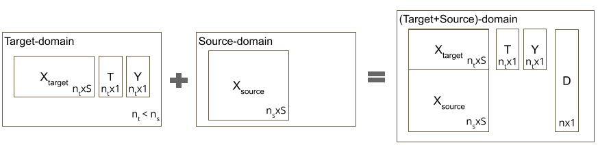
Causal-Batle is a treatment effect estimator for observational studies. We assume two domains: the target-domain and the source-domain. The target-domain is the small high-dimensional dataset we extract the treatment effect from, and it is composed of covariates , a binary treatment assignment , and continuous outcome . The source-domain contains the covariates , which are from the same feature space as . Here, we assume the source-domain is unlabeled (without treatment assignment or outcomes). Consider , and , where and are the sample sizes of the source-domain and target-domain, respectively. We create a new binary variable , which encodes the sample’s domain. We define the target-domain set as and .
The individual treatment effect (ITE) for a given sample is defined as , where is the potential outcomes under . The challenge is each sample either has a or associated, never both. A solution is to work with the Average Treatment Effect (ATE), the focus of our work, defined as . We define outcome models as , and estimate ATE as .
3.2 Assumptions
In this section, we list the underlying assumptions of Causal-Batle. To illustrate our methodology, we adopt a dragonnet architecture [19] as the backbone of our neural network. Other backbones architecture could also be adopted, such as convolutional neural networks for image-based applications.
Assumption 1: The target-domain covariates and source-domain covariates are in the same feature space.
Assumption 2: Stable Unit Treatment Value Assumption (SUTVA) [17] - the response of a particular unit depends only on the treatment(s) assigned, not the treatments of other units.
Assumption 3: Ignorability - the outcome is independent of the treatment given the covariates ().
Definition 1: Back-door Criterion [13] - Given a pair of variables in a directed acyclic graph , a set of variables satisfies the backdoor criterion relative to if no node in is a descendant of , and blocks every path between and that contains an arrow into .
Theorem 1: Identifiability [13] - If a set of variables satisfies the back-door criterion relative to , then the causal effect of on is identifiable.
Assumption 1 is related to our TL component to ensure both domains share the same features. According to Assumption 2, our target-domain is generated as , where is the observational distribution of the target-domain. Assumption 2 is also a standard causal inference assumption, which guarantees that one unit does not affect other units. According to Assumption 3, the observed covariates contain all the confounders of the treatment and outcome . Assumption 3 guarantees that will block all back-door paths and satisfy the back-door criterion (Definition 1). Thus, the identifiability of the treatment effect is guaranteed by Theorem 1. Note that we assume a setting with strong ignorability (Assumption 3). If that is not the case, one might need to choose a different backbone architecture and make extra assumptions to guarantee identifiability. However, while there are recent works exploring how to estimate treatment effects with unobserved confounders [20, 12, 11, 22], they still have several known limitations [15, 24]. Furthermore, working with unobserved confounders is not the focus of this paper.
Theorem 2: Sufficiency of Propensity Score [16, 19] - If the average treatment effect is identifiable from observational data by adjusting for , i.e., , then adjusting for the propensity score also suffices:
According to the Sufficiency of Propensity Score, it suffices to use only the information in relevant to predicting the propensity score, . The propensity score is predicted by , and all the relevant information to predict is the output of . For the proof, please refer to the original publication Rosenbaum and Rubin [16].
3.3 Architecture
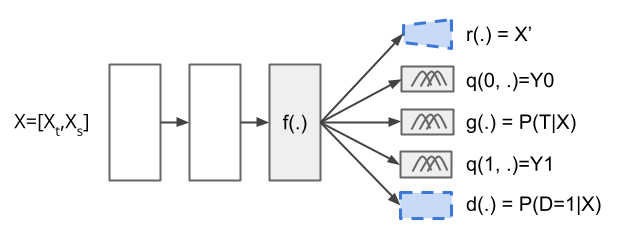
Causal-Batle builds upon existing neural network methods that estimate treatment effects. While not tied to any specific architecture, we will explain our methodology using a Dragonnet [19] as a backbone. The Dragonnet is a neural network with three heads: one to predict the treatment assignment given the input features, and the other two to predict the outcome if treated and untreated. It assumes no hidden confounders and relies on the Sufficiency of Propensity Score (Theorem 1) to estimate its outcomes, later used to estimate the treatment effects. The Dragonnet architecture has five key components: a shared representation of the input covariates , treatment assignment prediction , a targeted regularization, and the prediction of the outcome if treated and untreated. Jesson et al. [7] showed that for high-dimensional datasets, Bayesian neural networks tend to yield better results than their non-Bayesian neural network counterpart. They proposed a modification that suits most treatment effect estimators based on neural networks: a Gaussian mixture on the last layer.
| (1) |
where , , and are the observed outcome, the treatment assigned, and the covariates, respectively, and are the neural network weights.
Up to this point, all components of the architecture address only the estimation of the outcome in a high-dimensional setting. Note that these components assume the sample size is sufficiently large to train such a neural network. It is also worth noticing that, regardless of the backbone adopted (in our case, Dragonnet), training the shared representation is the most expensive step: this is the component with the largest number of weights, which receives as input the high-dimensional data and outputs a lower-dimensional representation of that data, used as input by the other components.
Causal-Batle focuses on improving the training of , the hardest part of the architecture. The idea is to use the source-domain to improve the representation of (hence, transfer knowledge from source-domain to target-domain). With a better trained , the estimation of the outcome models and the propensity score would yield better results.
Causal-Batle adds two new components to the network architecture: a discriminator and a reconstruction layer , and their corresponding terms in the loss function. The overall architecture is shown in Figure 2, with the two new components highlighted with blue-traced boards. The discriminator component is a binary classifier defined as . Therefore, for a given sample , the discriminator will predict whether it belongs to the source or target-domain. The adversarial loss incentives to extract patterns common to both domains and fool . The adversarial loss also helps remove spurious correlations and potential biases present in only one of the domains, improving ’s representation. The reconstruction component is to ensure ’s representation is meaningful. For the reconstruction component , in our work, we adopt an autoencoder for simplicity, but we point out that one could replace it with more sophisticated methods, such as variational autoencoders.
Similarly to Jesson et al. [7], Causal-Batle adopts a Bayesian neural network with a Gaussian Mixture for the outcomes (See Equation 1), and for the propensity score, with a Bernoulli Distribution:
| (2) |
Causal-Batle does not assume a distribution for the discriminator . Instead, it adopts a neural network classification node, which allows it to use traditional losses for adversarial learning.
3.4 Loss Functions
The exact loss function will depend on the backbone architecture adopted. Here, we will present the loss function for the example given in Figure 2, which is a bayesian dragonnet architecture. Note that we have samples in the target-domain, samples in the source-domain, and
There is a loss associated with each grey/blue square. Starting with the outcome model loss: we only observe the outcome for either or , with representing a distribution. Therefore, we define the loss as the log probability:
| (3) |
The propensity score loss is also calculated using log probability.
| (4) |
To capture the losses associated with the transfer learning components, we adopt a second binary cross entropy loss for the discriminator. Defining :
| (5) |
and to compete with the discriminator loss, we have the adversarial loss:
| (6) |
Finally, the reconstruction loss ensures the features extracted by are meaningful. Denoting by the reconstruction of input , we have:
| (7) |
The final loss is defined as:
| (8) |
where the array are the losses’ weights.
3.5 Treatment Effect Estimation
3.6 Source-domain and Target-domain relationship
This section discusses the relationship between the source and target-domain. Causal-Batle aims to use the unlabeled source-domain to learn a better representation of the labeled target-domain. There are three losses associated with the transfer learning: the discriminator loss , the adversarial loss , and the reconstruction loss . Here, we discuss the impact of (target-domain distribution) and (source-domain distribution) in our proposed methodology.
-
•
: will be large, as the discriminator will have a hard time trying to distinguish elements from two identical distributions while working against the adversarial loss. The loss, on the other hand, will thrive. A large collection of samples from the same distribution will help to find a good representation of the input data, lowering the .
-
•
: will be low, as would be able to identify these differences and use them. Still, would attempt to fool , which would push to learn a domain agnostic representation.
This means that, in practice, regardless of the and distributions, the losses would push to have a meaningful representation of . The key is to find a balance between the adversarial loss, the discriminator loss, and the reconstruction loss, which, as shown in Equation 8 is controlled by the weights (hyper-parameters) .
4 Experiments
Our experiments compare Causal-Batle against some of the most adopted causal inference baselines for binary treatments: Dragonnet [19], Bayesian Dragonnet [7], AIPW [4], and CEVAE [11]. Note that none of these baselines adopt transfer-learning techniques. The main questions we want to investigate are:
-
•
Does the transfer learning approach improve the treatment effect estimates compared to existing treatment effect methods?
-
•
What is the impact of the ratio between the sizes of (unlabeled source-domain) and (labeled target-domain)?
To make a fair comparison between Causal-Batle and the baselines, we adopt the following scheme:
Setting 1 - Datasets with only : In the evaluation, we also adopted traditional benchmark datasets, which do not have an unlabeled source domain. To adapt to our setting, we splited the samples of into two sets: samples to and samples to . The quantity represents the proportion of the dataset used as target-domain, with . We removed the labels (treatment assignment and outcome) from the samples in . The baselines receive the labeled target-dataset , and Causal-Batles receives the target-dataset and the unlabeled source-dataset .
Setting 2 - Datasets with and : Baselines are trained using only . Causal-Batle would have access to both domains.
We define the ratio as , representing the target-domain’s size relative to the source-domain. The Causal-Batle ideal use-cause is for applications with low . The code to an implemented version of Causal-Batle is available at github/HiddenForDoubleBlindSubmission. We simulated each dataset times and fitted each method times. Therefore, each given combination of (dataset method) was repeated times for consistency and reproducibility. For the Causal-Batle, Dragonnet, and Bayesian Dragonnet, we adopted the same backbone architecture to have a fair comparison. As metric, we adopt the Mean Absolute Error (MAE) between the estimated treatment effect and the true treatment effect , defined as . In our plots and tables, we report the average value over all the repetitions: . Low values of MAE are desirable. The experiments were run using GPUs on Colab Pro+.
4.1 Datasets
We adopted the three datasets to validate our proposed method. Please check our Appendix for an extended description of the datasets:
GWAS [22, 1]: The Genome-Wide Association Study (GWAS) dataset is a semi-simulated dataset that explores sparse settings. Proposed initially to handle multiple treatments, we adapt it to have one binary treatment and a continuous outcome . We split the data into two datasets, as explained in Setting 1. Note that and have the same distribution. We simulated a small high-dimensional dataset with 2k samples and 10k covariates.
IHDP[6]: The Infant Health and Development Program (IHDP) is a popular causal inference semi-synthetic benchmark dataset with binary treatment and continuous outcome. This dataset has ten repetitions, with 23 covariates and approximately 747 samples. We adopted Setting 1. Note that this dataset is not high-dimensional; still, it is a classic dataset in Causal Inference.
CMNIST [8]: A semi-synthetic dataset that adapts the MNIST [10] dataset to causal inference. It contains a binary treatment and continuous outcome. We follow the setup from Jesson et al. [8] with small adaptations to contain a source and a target-domain. Jesson et al. [8] generates the treatment assignments and the outcomes partially based on the images’ representation. In our adaption, we also follow this scheme, but we only used two randomly selected digits . Therefore, in our target-domain, we have the images of the digits and . We map the high-dimensional images to a one-dimensional array (See Appendix for more details), which is used to simulate the treatments and the outcome . For the source-domain, we use the images of the other digits. As the source-domain is unlabeled, there is no treatment or outcome produced, and we use the images as they are observed. We follow Setting 2.
4.2 Experimental Results
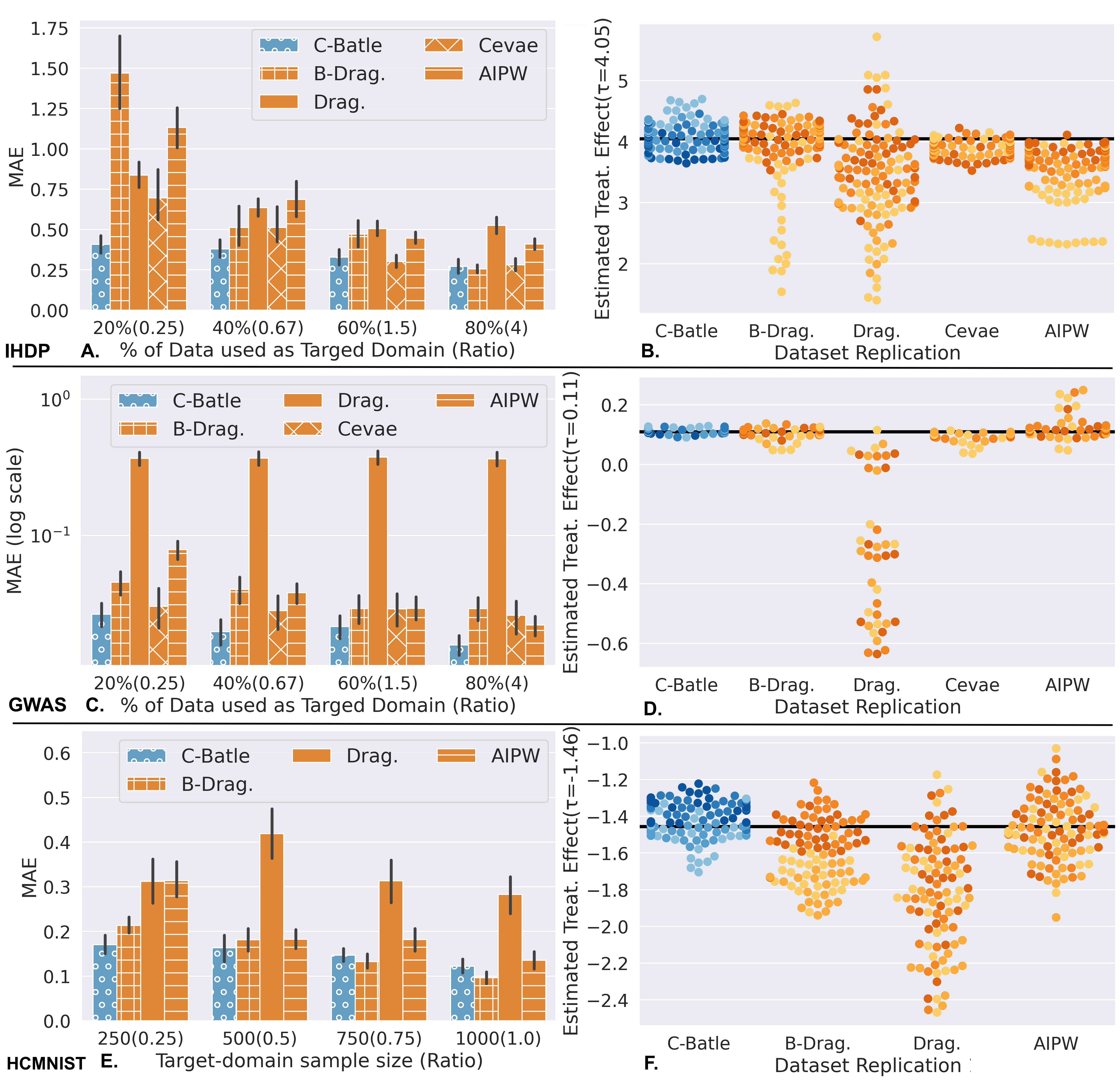
Setting 1 (Figure 3A-D): We explored the following ratios , with low being the ideal use-case of Causal-Batle. For the IHDP dataset, we adopted datasets replications with model repetitions, for a total of estimated values for each . For the GWAS dataset, we adopted dataset replications with model repetitions for each (). The IHDP dataset is not a small high-dimensional dataset; however, it is a classic benchmark dataset. With , Causal-Batle outperforms all the other baselines as shown in Figure 3.A. With , the performance of all methods improves, including Causal-Batle, which stays in the top 2. Figure 3.B shows the model repetitions on a dataset replication, where the colors indicate the value (lighter colors low ). Besides having the lowest MAE’s, Causal-Batle estimations are well distributed around the true value, while some baselines often underestimate the true values, especially for low values (light-colored dots).
The GWAS dataset fits more in our ideal use-case, containing 2k samples and 10k covariates. As a reminder, means that all methods will receive samples as , which contains the treatment assignment and the outcome of interest; Causal-Batle, on top of the , also receives , which contains unlabeled samples (only covariates available, without treatment assignment nor outcome). Figure 3.C shows that Causal-Batle has the lowest MAE among all methods considered, with the distance between Causal-Batle and the other methods decreasing as increases. Figure 3.D shows that Causal-Batle estimated values are well distributed around the true value. Note that the Bayesian Dragonnet and CEVAE are also well distributed around the true value; however, they underestimate with low values.
Setting 2 (Figure 3E-F): The HCMNIST had dataset replications and model repetitions, for a total of estimated values for each . As Figure 3.E shows, Causal-Batle has the smallest MAE for , and the second-best MAE for . According to the experimental results in Figure 3.F, both Causal-Batle and the Bayesian Dragonnet tend to underestimate the treatment effect with low values (light colors). However, Causal-Batle has lower variance, and its estimates are more accurate than Bayesian Dragonnet’s estimates.
Discussion: Causal-Batle has more accurate estimates (low MAE) than the baselines for low values. Note that the only difference between Causal-Batle and the Bayesian Dragonnet is the transfer learning components (discriminator loss, adversarial loss, reconstruction loss, and the use of the dataset). An explanation for these results is that transfer learning improves the estimates. Considering the IHDP dataset, when , the simpler architecture of the Bayesian Dragonnet performs better, indicating a possible threshold for the IHDP dataset when a simpler architecture is preferable over a more complex one with transfer learning. For the GWAS and HCMNIST datasets, that threshold is above and . Note that we did not experiment with CEVAE with the HCMNIST as that would require many changes to the CEVAE to work with image data, which was not our focus. Finally, we investigated Dragonnet’s poor performance. Our main hypothesis is that the Bayesian component included in the Bayesian Dragonnet and Causal-Batle reduces the variability and improves estimates. The Bayesian component predicts the outcome and the treatment assignment as a Gaussian Mixture and Bernoulli distribution, respectively, and predictions are calculated using MC-dropout (30 forward passes).
5 Conclusion
This paper addresses an important and underexplored problem: causal inference in small high-dimensional datasets. In Section 2 we describe existing approaches to estimate treatment effects with a binary treatment and continuous outcome, along with their main limitations. We later describe in Section 3 our assumptions and our proposed method, Causal-Batle, and the main characteristics of the target and source-domain datasets. Finally, in Section 4 we validate our method, comparing it with existing methods in three different datasets. The Causal-Batle ideal use case is tested in our experiments when we have low . Under this setting, Causal-Batle has the best performance among all the baselines considered. In other settings, with larger target-domain datasets, the performance is comparable to the baselines. Therefore, according to our experimental results, the transfer learning components of Causal-Batle improved the treatment effect estimations for low values of compared to other methods.
Causal-Batle, like other machine learning methods, could have negative societal impacts if misused, fed biased data, or applied to unethical applications. In general, we believe most Causal-Batle negative characteristics are inherent to the field (of machine learning) rather than our proposed method. Ethics guidelines can help reduce unethical applications while the others can be mitigated by increasing the transparency in methodologies, datasets, and code availability. Causal-Batle’s dependence on the availability of an unlabeled source-domain dataset in the same feature space as the target-domain dataset can be considered a limitation of our approach, along with the strong ignorability assumption that is often difficult to guarantee in real-world applications. To address the first limitation, we recommend checking the baselines adopted by our work, in particular the Bayesian Dragonnet[7] and CEVAE[11], as these two methods do not need external source-domain datasets. As for the strong ignorability assumption, one might adopt a sensitivity analysis [21] to investigate the impact of unobserved confounders on the estimation of treatment effects.
Overall, Causal-Batle demonstrated to be a good estimator for its intended use case. Such a setting is very common in Computational Biology applications, where we often have high-dimensional datasets with genetic information but a limited number of samples available with treatment assignment and observed outcome. Yet, several unlabeled datasets in the same feature space could be used under certain assumptions to improve causal inference in small high-dimensional datasets. Another use-case example is when images are used as covariates to perform causal inference - a topic that has recently received more attention. In this case, if only a few labeled images are available to estimate the treatment effects, one could adopt several unlabeled (similar) images to improve the feature extraction component of Causal-Batle, and, consequently, improve the treatment effect estimation.
References
- Aoki and Ester [2021] Raquel Aoki and Martin Ester. Parkca: Causal inference with partially known causes. Pac Symp Biocomputing, 2021.
- Bareinboim and Pearl [2014] Elias Bareinboim and Judea Pearl. Transportability from multiple environments with limited experiments: Completeness results. Advances in neural information processing systems, 27:280–288, 2014.
- Chau et al. [2021] Siu Lun Chau, Jean-Francois Ton, Javier Gonzalez, Yee Whye Teh, and Dino Sejdinovic. BayesIMP: Uncertainty quantification for causal data fusion. In Thirty-Fifth Conference on Neural Information Processing Systems, 2021. URL https://openreview.net/forum?id=aSjbPcve-b.
- Glynn and Quinn [2010] Adam N Glynn and Kevin M Quinn. An introduction to the augmented inverse propensity weighted estimator. Political analysis, 18(1):36–56, 2010.
- Guo et al. [2021] Wenshuo Guo, Serena Wang, Peng Ding, Yixin Wang, and Michael I Jordan. Multi-source causal inference using control variates. arXiv preprint arXiv:2103.16689, 2021.
- Hill [2011] Jennifer L Hill. Bayesian nonparametric modeling for causal inference. Journal of Computational and Graphical Statistics, 20(1):217–240, 2011.
- Jesson et al. [2020] Andrew Jesson, Sören Mindermann, Uri Shalit, and Yarin Gal. Identifying causal-effect inference failure with uncertainty-aware models. Advances in Neural Information Processing Systems, 33, 2020.
- Jesson et al. [2021] Andrew Jesson, Sören Mindermann, Yarin Gal, and Uri Shalit. Quantifying ignorance in individual-level causal-effect estimates under hidden confounding. In International Conference on Machine Learning, page pages 4829–4838, 2021.
- Künzel et al. [2019] Sören R Künzel, Jasjeet S Sekhon, Peter J Bickel, and Bin Yu. Metalearners for estimating heterogeneous treatment effects using machine learning. Proceedings of the national academy of sciences, 116(10):4156–4165, 2019.
- LeCun [1998] Yann LeCun. The mnist database of handwritten digits. http://yann. lecun. com/exdb/mnist/, 1998.
- Louizos et al. [2017] Christos Louizos, Uri Shalit, Joris M Mooij, David Sontag, Richard Zemel, and Max Welling. Causal effect inference with deep latent-variable models. Advances in neural information processing systems, 30, 2017.
- Mastouri et al. [2021] Afsaneh Mastouri, Yuchen Zhu, Limor Gultchin, Anna Korba, Ricardo Silva, Matt J Kusner, Arthur Gretton, and Krikamol Muandet. Proximal causal learning with kernels: Two-stage estimation and moment restriction. Advances in Neural Information Processing Systems, 2021.
- Pearl [1995] Judea Pearl. Causal diagrams for empirical research. Biometrika, 82(4):669–688, 1995.
- Pearl and Bareinboim [2011] Judea Pearl and Elias Bareinboim. Transportability of causal and statistical relations: A formal approach. In Twenty-fifth AAAI conference on artificial intelligence, 2011.
- Rissanen and Marttinen [2021] Severi Rissanen and Pekka Marttinen. A critical look at the consistency of causal estimation with deep latent variable models. Advances in Neural Information Processing Systems, 34, 2021.
- Rosenbaum and Rubin [1983] Paul R Rosenbaum and Donald B Rubin. The central role of the propensity score in observational studies for causal effects. Biometrika, 70(1):41–55, 1983.
- Rubin [1980] Donald B Rubin. Randomization analysis of experimental data: The fisher randomization test comment. Journal of the American Statistical Association, 75(371):591–593, 1980.
- Shalit et al. [2017] Uri Shalit, Fredrik D Johansson, and David Sontag. Estimating individual treatment effect: generalization bounds and algorithms. In International Conference on Machine Learning, pages 3076–3085. PMLR, 2017.
- Shi et al. [2019] Claudia Shi, David Blei, and Victor Veitch. Adapting neural networks for the estimation of treatment effects. In Advances in Neural Information Processing Systems, pages 2503–2513, 2019.
- Tchetgen et al. [2020] Eric J Tchetgen Tchetgen, Andrew Ying, Yifan Cui, Xu Shi, and Wang Miao. An introduction to proximal causal learning. arXiv preprint arXiv:2009.10982, 2020.
- Veitch and Zaveri [2020] Victor Veitch and Anisha Zaveri. Sense and sensitivity analysis: Simple post-hoc analysis of bias due to unobserved confounding. Advances in Neural Information Processing Systems, 33:10999–11009, 2020.
- Wang and Blei [2019] Yixin Wang and David M Blei. The blessings of multiple causes. Journal of the American Statistical Association, (just-accepted), 2019.
- Yang and Ding [2019] Shu Yang and Peng Ding. Combining multiple observational data sources to estimate causal effects. Journal of the American Statistical Association, 2019.
- Zheng et al. [2021] Jiajing Zheng, Alexander D’Amour, and Alexander Franks. Copula-based sensitivity analysis for multi-treatment causal inference with unobserved confounding. arXiv preprint arXiv:2102.09412, 2021.
- Zhuang et al. [2020] Fuzhen Zhuang, Zhiyuan Qi, Keyu Duan, Dongbo Xi, Yongchun Zhu, Hengshu Zhu, Hui Xiong, and Qing He. A comprehensive survey on transfer learning. Proceedings of the IEEE, 109(1):43–76, 2020.
Appendix A Appendix
A.1 HCMNIST[8]
Proposed by Jesson et al. [8], it is an adaptation of the MNIST[10] dataset to causal inference. This dataset contains a binary treatment and continuous outcome. We follow the setup from Jesson et al. [8] with small adaptations to contain a source and a target-domain. In our adaption, we randomly pick two digits to be our target-domain, and we use another randomly chosen digit to be our source-domain. As the source-domain is unlabeled, there is no treatment or outcome produced. Note that, while the digits are used to generate the data, the treatment is not the digit in the image.
For each sample (target-domain), we have the corresponding digit (). The semi-synthetic dataset is constructed as follows:
-
1.
For each digit selected for the target-domain, we calculate the average intensity across all images and standard deviation .
-
2.
The average intensity of a sample is defined as ;
-
3.
The high-dimensional images are mapped into a one-dimensional manifold . The images intensity are also standardized on the range ;
-
4.
There is a linear transformation for each digit in the target-domain, defined by ; As we have two digits, we adopted for and for .
Finally, , and can be calculated as follows:
where .
A.2 GWAS
We followed a standard GWAS dataset[song2015testing, 22, 1]. Similar to existing works, the covariates and treatments are single-nucleotide polymorphisms (SNPs). The target variable also referred to as the outcome of interest, is continuous. The main difference between Causal-Batle GWAS and the others is that in this work, we adopted only one SNP as a treatment. In contrast, most of the existing works explore multiple treatment settings.
-
1.
The 1000 Genome Project (TGP) is used as allele Frequency , where is the number of samples and the number of SNPs.
-
2.
We remove highly correlated SNPs using linkage disequilibrium.
-
3.
: it extracts principal components from a PCA fitted to the TGP data base ().
-
4.
We append a new column to such that is the intercept.
-
5.
The matrix represents the simulated samples:
(10) and
-
6.
The matrix of allele frequency is obtained from .
-
7.
is used to simulate the covariates:
(11) -
8.
We randomly pick one item in to be the treatment. We set for the SNP used as a treatment, and .
-
9.
The treatment effect is simulated as .
-
10.
To add confounding effect, the samples are grouped using and three clusters . These clusters are used as per-group intercept and to define the error variance , where .
-
11.
Following a high signal-to-noise ration, the SNP’s and the per-group intercept are responsible for 40% () of the variance each, and the error is responsible for 20% () of the variance. To re-scale the noise and intercept:
(12) (13) -
12.
Finally, the outcomes are generated as:
(14)