date origdate n.d.
Causality in cognitive neuroscience: concepts, challenges, and distributional robustness
Abstract
While probabilistic models describe the dependence structure between observed variables, causal models go one step further: they predict, for example, how cognitive functions are affected by external interventions that perturb neuronal activity. In this review and perspective article, we introduce the concept of causality in the context of cognitive neuroscience and review existing methods for inferring causal relationships from data. Causal inference is an ambitious task that is particularly challenging in cognitive neuroscience. We discuss two difficulties in more detail: the scarcity of interventional data and the challenge of finding the right variables. We argue for distributional robustness as a guiding principle to tackle these problems. Robustness (or invariance) is a fundamental principle underlying causal methodology. A causal model of a target variable generalises across environments or subjects as long as these environments leave the causal mechanisms intact. Consequently, if a candidate model does not generalise, then either it does not consist of the target variable’s causes or the underlying variables do not represent the correct granularity of the problem. In this sense, assessing generalisability may be useful when defining relevant variables and can be used to partially compensate for the lack of interventional data.
1 Introduction
Cognitive neuroscience aims to describe and understand the neuronal underpinnings of cognitive functions such as perception, attention, or learning. The objective is to characterise brain activity and cognitive functions, and to relate one to the other. The submission guidelines for the Journal of Cognitive Neuroscience, for example, state: “The Journal will not publish research reports that bear solely on descriptions of function without addressing the underlying brain events, or that deal solely with descriptions of neurophysiology or neuroanatomy without regard to function.” We think that understanding this relation requires us to relate brain events and cognitive function in terms of the cause-effect relationships that govern their interplay. A causal model could, for example, describe how cognitive functions are affected by external interventions that perturb neuronal activity (cf. Section 2.1). [86] argue that “the ultimate phenomenon of theoretical interest in all FC [functional connectivity] research is understanding the causal interaction among neural entities”.
Causal inference in cognitive neuroscience is of great importance and perplexity. This motivates our discussion of two pivotal challenges. First, the scarcity of interventional data is problematic as several causal models may be equally compatible with the observed data while making conflicting predictions only about the effects of interventions (cf. Section 3.1). Second, the ability to understand how neuronal activity gives rise to cognition depends on finding the right variables to represent the neuronal activity (cf. Section 3.2). Our starting point is the well-known observation that causal models of a target (or response) variable are distributionally robust and thus generalise across environments, subjects, and interventional shifts [37, 1, 71]. Models that do not generalise are either based upon the wrong variables that do not represent causal entities or include variables that are not causes of the target variable. We thus propose to pursue robust (or invariant) models. That way, distributional robustness may serve as a guiding principle towards a causal understanding of cognitive function and may help us tackle both challenges mentioned above.
1.1 Running examples
We consider the following simplified examples. Assume that the consumption of alcohol affects reaction times in a cognitive task. In a randomised controlled trial we find that drinking alcoholic (versus non-alcoholic) beer results in slowed reaction times hereinafter. Therefore, we may write ‘’ and call alcohol a cause of reaction time and reaction time an effect of alcohol. Intervening on the cause results in a change in the distribution of the effect. In our example, prohibiting the consumption of any alcoholic beers results in faster reaction times.
In cognitive neuroscience one may wish to describe how the neuronal activity is altered upon beer consumption and how this change in turn affects the reaction time. For this, we additionally require a measurement of neuronal activity, say a functional magnetic resonance imaging (fMRI) scan and voxel-wise blood-oxygen-level dependent (BOLD) signals, that can serve as explanans in a description of the phenomenon ‘’. We distinguish the following two scenarios:
Running Example A, illustrated in Figure 1(a).
A so-called treatment or stimulus variable (say, consumption of alcohol) affects neuronal activity as measured by a -dimensional feature vector and the target variable reflects a cognitive function (say, reaction time). We may concisely write for a treatment that affects neuronal activity which in turn maintains a cognitive function [[, this is analogous to the ‘stimulus brain activity response’ set-up considered in]]weichwald2014causal,weichwald2015causal.
Running Example B, illustrated in Figure 1(b).
We may wish to describe how neuronal entities cause one another and hence designate one such entity as the target variable . In this example, we consider a target variable corresponding to a specific brain signal or region instead of a behavioural or cognitive response.
1.2 Existing work on causality in the context of cognitive neuroscience
Several methods such as Granger causality or constraint-based methods have been applied to the problem of inferring causality from cognitive neuroscience data. We describe these methods in Section 2.3. In addition, there are ongoing conceptual debates that revolve around the principle of causality in cognitive neuroscience, some of which we now mention. [65] raise concerns about the “lure of causal statements” and expound the problem of confounding when interpreting functional connectivity. Confounders are similarly problematic for multi-voxel pattern analyses [106, 122]. The causal interpretation of encoding and decoding (forward and backward, univariate and multivariate) models has received much attention as they are common in the analysis of neuroimaging data: [25] examine the differences between the model types, [38] point out that the weights of linear backward models may be misleading, and [119] extend the latter argument to non-linear models and clarify which causal interpretations are warranted from either model type. Feature relevance in mass-univariate and multivariate models can be linked to marginal and conditional dependence statements that yield an enriched causal interpretation when both are combined [119]; this consideration yields refined results in neuroimaging analyses [45, 3, 112] and explains improved functional connectivity results when combining bivariate and partial linear dependence measures [89]. Problems such as indirect measurements and varying temporal delays complicate causal Bayesian network approaches for fMRI [83, 68]. [99] present a simulation study evaluating several methods for estimating brain networks from fMRI data and demonstrate that identifying the direction of network links is difficult. The discourse on how to leverage connectivity analyses to understand mechanisms in brain networks is ongoing [110, 115, 98, 66]. Many of the above problems and findings are related to the two key challenges that we discuss in Section 3.
1.3 Structure of this work
We begin Section 2 by formally introducing causal concepts. In Section 2.1, we outline why we believe there is a need for causal models in cognitive neuroscience by considering what types of questions could be answered by an OraCle Modelling (OCM) approach. We discuss the problem of models that are observationally equivalent yet make conflicting predictions about the effects of interventions in Section 2.2. In Section 2.3, we review different causal discovery methods and their underlying assumptions. We focus on two challenges for causality in cognitive neuroscience that are expounded in Section 3: (1) the scarcity of interventional data and (2) the challenge of finding the right variables. In Section 4, we argue that one should seek distributionally robust variable representations and models to tackle these challenges. Most of our arguments in this work are presented in an i.i.d. setting and we briefly discuss the implications for time-dependent data in Section 4.5. We conclude in Section 5 and outline ideas that we regard as promising for future research.
2 Causal models and causal discovery
In contrast to classical probabilistic models, causal models induce not only an observational distribution but also a set of so-called interventional distributions. That is, they predict how a system reacts under interventions. We present an introduction to causal models that is based on pioneer work by [71] and [100]. Our exposition is inspired by [116, Chapter 2], which provides more introductory intuition into causal models viewed as structured sets of interventional distributions. For both simplicity and focus of exposition, we omit a discussion of counterfactual reasoning and other akin causality frameworks such as the potential outcomes formulation of causality [47]. We phrase this article within the framework and terminology of Structural Causal Models (SCMs) [9, 71].
An SCM over variables consists of
- structural equations
-
that relate each variable to its parents and a noise variable via a function such that , and a
- noise distribution
-
of the noise variables .
We associate each SCM with a directed causal graph where the nodes correspond to the variables and we draw an edge from to whenever appears on the right hand side of the equation . That is, if the graph contains the edge . Here, we assume that this graph is acyclic. The structural equations and noise distributions together induce the observational distribution of as simultaneous solution to the equations. ([10] formally define SCMs when the graph includes cycles.)
The following is an example of a linear Gaussian SCM:
with mutually independent standard-normal noise variables . The corresponding graph is
and the SCM induces the observational distribution , which is the multivariate Gaussian distribution
| (1) |
In addition to the observational distribution, an SCM induces interventional distributions. Each intervention denotes a scenario in which we fix a certain subset of the variables to a certain value. For example, the intervention denotes the scenario where we force and to take on the values and , respectively. The interventional distributions are obtained by (a) replacing the structural equations of the intervened upon variables by the new assignment, and (b) considering the distribution induced by the thus obtained new set of structural equations. For example, the distribution under intervention for , denoted by , is obtained by changing the equation to . In the above example, we find
where if and only if . Analogously, for and intervention on we have
The distribution of differs between the observational distribution and the interventional distribution, that is, . We call a variable an (indirect) cause of a variable if there exists an intervention on under which the distribution of is different from its distribution in the observational setting. Thus, is a cause of . The edge in the above causal graph reflects this cause-effect relationship. In contrast, remains standard-normally distributed under all interventions on . Because the distribution of remains unchanged under any intervention on , is not a cause of .
In general, interventional distributions do not coincide with the corresponding conditional distributions. In our example we have while . We further have that the conditional distribution of given its parents and is invariant under interventions on variables other than . We call a model of based on invariant (cf. Section 4.1).
We have demonstrated how an SCM induces a set of observational and interventional distributions. The interventional distributions predict observations of the system upon intervening on some of its variables. As such, a causal model holds additional content compared to a common probabilistic model that amounts to one distribution to describe future observations of the same unchanged system. Sometimes we are only interested in modelling certain interventions or cannot perform others as there may be no well-defined corresponding real-world implementation. For example, we cannot intervene on a person’s gender. In these cases it may be helpful to explicitly restrict ourselves to a set of interventions of interest. Furthermore, the choice of an intervention set puts constraints on the granularity of the model [*][cf. Section 3.2 and Rubenstein & Weichwald et al.,][]rubenstein2017causal.
2.1 When are causal models important?
We do not always need causal models to answer our research question. For some scientific questions it suffices to consider probabilistic, that is, observational models. For example, if we wish to develop an algorithm for early diagnosis of Alzheimer’s disease from brain scans, we need to model the conditional distribution of Alzheimer’s disease given brain activity. Since this can be computed from the joint distribution, a probabilistic model suffices. If, however, we wish to obtain an understanding that allows us to optimally prevent progression of Alzheimer’s disease by, for example, cognitive training or brain stimulation, we are in fact interested in a causal understanding of the Alzheimer’s disease and require a causal model.
Distinguishing between these types of questions is important as it informs us about the methods we need to employ in order to answer the question at hand. To elaborate upon this distinction, we now discuss scenarios related to our running examples and the relationship between alcohol consumption and reaction time (cf. Section 1.1). Assume we have access to a powerful OraCle Modelling (OCM) machinery that is unaffected by statistical problems such as model misspecification, multiple-testing, or small sample sizes. By asking ourselves, what queries must be answered by OCM for us to ‘understand’ the cognitive function, the difference between causal and non-causal questions becomes apparent.
Assume, firstly, we ran the reaction task experiment with multiple subjects, fed all observations to our OCM machinery, and have Kim visiting our lab today. Since OCM yields us the exact conditional distribution of reaction times for Kim having consumed units of alcoholic beer, we may be willing to bet against our colleagues on how Kim will perform in the reaction task experiment they are just about to participate in. No causal model for brain activity is necessary.
Assume, secondly, that we additionally record BOLD responses at certain locations and times during the reaction task experiment. We can query OCM for the distribution of BOLD signals that we are about to record, that is, , or the distribution of reaction times given we measure Kim’s BOLD responses , that is, . As before, we may bet against our colleagues on how Kim’s BOLD signals will look like in the upcoming reaction task experiment or bet on their reaction time once we observed the BOLD activity prior to a reaction cue. Again, no causal model for brain activity is required.
In both of the above situations, we have learned something useful. Given that the data were obtained in an experiment in which alcohol consumption was randomised, we have learned, in the first situation, to predict reaction times after an intervention on alcohol consumption. This may be considered an operational model for alcohol consumption and reaction time. In the second situation, we have learned how the BOLD signal responds to alcohol consumption. Yet, in none of the above situations have we gained understanding of the neuronal underpinnings of the cognitive function and the reaction times. Knowing the conditional distributions and for any yields no insight into any of the following questions. Which brain regions maintain fast reaction times? Where in the brain should we release drugs that excite neuronal activity in order to counterbalance the effect of alcohol? How do we need to update our prediction if we learnt that Kim just took a new drug that lowers blood pressure in the prefrontal cortex? To answer such questions, we require causal understanding.
If we had a causal model, say in form of an SCM, we could address the above questions. An SCM offers an explicit way to model the system under manipulations. Therefore, a causal model can help to answer questions about where to release an excitatory drug. It may enable us to predict whether medication that lowers blood pressure in the prefrontal cortex will affect Kim’s reaction time; in general, this is the case if the corresponding variables appear in the structural equations for or any of ’s ancestors.
Instead of identifying conditional distributions, one may formulate the problem as a regression task with the aim to learn the conditional mean functions and . These functions are then parameterised in terms of or and . We argue in Section 2.2, point (2), that such parameters do not carry a causal meaning and thus do not help to answer the questions above.
Promoted by slogans such as ‘correlation does not imply causation’ careful and associational language is sometimes used in the presentation of cognitive neuroscience studies. We believe, however, that a clear language that states whether a model should be interpreted causally (that is, as an interventional model) or non-causally (that is, as an observational model) is needed. This will help to clarify both the real world processes the model can be used for and the purported scientific claims.
Furthermore, causal models may generalise better than non-causal models. We expect systematic differences between subjects and between different trials or recording days of the same subject. These different situations, or environments, are presumably not arbitrarily different. If they were, we could not hope to gain any scientific insight from such experiments. The apparent question is, which parts of the model we can expect to generalise between environments. It is well-known that causal models capture one such invariance property, which is implicit in the definition of interventions. An intervention on one variable leaves the assignments of the other variables unaffected. Therefore, the conditional distributions of these other variables, given their parents, are also unaffected by the intervention [37, 1]. Thus, causal models may enable us to formulate more clearly which mechanisms we assume to be invariant between subjects. For example, we may assume that the mechanism how alcohol intake affects brain activity differs between subjects, whereas the mechanism from signals in certain brain regions to reaction time is invariant. We discuss the connection between causality and robustness in Section 4.
2.2 Equivalences of models
Causal models entail strictly more information than observational models. We now introduce the notion of equivalence of models [71, 76, 10]. This notion allows us to discuss the falsifiability of causal models, which is important when assessing candidate models and their ability to capture cause-effect relationships that govern a cognitive process under investigation.
We call two models observationally equivalent if they induce the same observational distribution. Two models are said to be interventionally equivalent if they induce the same observational and interventional distributions. As discussed above, for some interventions there may not be a well-defined corresponding experiment in the real world. We therefore also consider interventional equivalence with respect to a restricted set of interventions.
One reason why learning causal models from observational data is difficult is the existence of models that are observationally but not interventionally equivalent. Such models agree in their predictions about the observed system yet disagree in their predictions about the effects of certain interventions. We continue the example from Section 2 and consider the following two SCMs:
where in both cases are mutually independent standard-normal noise variables. The two SCMs are observationally equivalent as they induce the same observational distribution, the one shown in Equation (1). The models are not interventionally equivalent, however, since and for the left and right model, respectively. The two models can be told apart when interventions on or are considered. They are interventionally equivalent with respect to interventions on .
The existence of observationally equivalent models that are not interventionally equivalent has several implications. (1) Without assumptions, it is impossible to learn causal structure from observational data. This is not exclusive to causal inference from data and an analogous statement holds true for regression [36]. The regression problem is solvable only under certain simplicity assumptions, for example, on the smoothness of the regression function, which have been proven useful in real world applications. Similarly, there are several assumptions that can be exploited for causal discovery. We discuss some of these assumptions in Section 2.3. (2) As a consequence, without further restrictive assumptions on the data generating process, the estimated parameters do not carry any causal meaning. For example, given any finite sample from the observational distribution, both of the above SCMs yield exactly the same likelihood. Therefore, the above structures cannot be told apart by a method that employs the maximum likelihood estimation principle. Instead, which SCM and thus which parameters are selected in such a situation may depend on starting values, optimisation technique, or numerical precision. (3) Assume that we are given a probabilistic (observational) model of a data generating process. To falsify it, we may apply a goodness-of-fit test based on an observational sample from that process. An interventional model cannot be falsified based on observational data alone and one has to also take into account the outcome of interventional experiments. This requires that we are in agreement about how to perform the intervention in practice (see also Section 3.2). Interventional data may be crucial in particular for rejecting some of the observationally equivalent models (cf. the example above). The scarcity of interventional data therefore poses a challenge for causality in cognitive neuroscience (cf. Section 3.1).
2.3 Causal discovery
The task of learning a causal model from observational (or a combination of observational and interventional) data is commonly referred to as causal discovery or causal structure learning. We have argued in the preceding section that causal discovery from purely observational data is impossible without any additional assumptions or background knowledge. In this section, we discuss several assumptions that render (parts of) the causal structure identifiable from the observational distribution. In short, assumptions concern how causal links manifest in observable statistical dependences, functional forms of the mechanisms, certain invariances under interventions, or the order of time. We briefly outline how these assumptions can be exploited in algorithms. Depending on the application at hand, one may be interested in learning the full causal structure as represented by its graph or in identifying a local structure such as the causes of a target variable . The methods described below cover either of the two cases. We keep the description brief focussing on the main ideas and intuition, while more details can be found in the respective references.
Randomisation.
The often called ‘gold standard’ to establishing whether causes is to introduce controlled perturbations, that is, targeted interventions, to a system. Without randomisation, a dependence between and could stem from a confounder between and or from a causal link from to . If is randomised it is no further governed by the outcome of any other variable or mechanism. Instead, it only depends on the outcome of a randomisation experiment, such as the roll of a die. If we observe that under the randomisation, depends on , say the higher the higher , then there must be a (possibly indirect) causal influence from to . In our running examples, this allows us to conclude that the amount of alcoholic beer consumed causes reaction times (cf. Section 1.1). When falsifying interventional models, it suffices to consider randomised experiments as interventions [[]Proposition 6.48]peters2017elements. In practice, however, performing randomised experiments is often infeasible due to cost or ethical concerns, or impossible as, for example, we cannot randomise gender nor fully control neuronal activity in the temporal lobe. While it is sometimes argued that the experiment conducted by James Lind in 1747 to identify a treatment for scurvy is among the first randomised controlled trials, the mathematical theory and methodology was popularised by Ronald A. Fisher in the early 20th century [22].
Constraint-based methods.
Constraint-based methods rely on two assumptions that connect properties of the causal graph with conditional independence statements in the induced distribution. The essence of the first assumption is sometimes described as Reichenbach’s common cause principle [85]: If and are dependent, then there must be some cause-effect structure that explains the observed dependence, that is, either causes , or causes , or another unobserved variable causes both and , or some combination of the aforementioned. This principle is formalised by the Markov condition [[, see for example]]Lauritzen1996. This assumption is considered to be mild. Any distribution induced by an acyclic SCM satisfies the Markov condition with respect to the corresponding graph [52, 71]. The second assumption (often referred to as faithfulness), states that any (conditional) independence between random variables is implied by the graph structure [100]. For example, if two variables are independent, then neither does cause the other nor do they share a common cause. Both assumptions together establish a one-to-one correspondence between conditional independences in the distribution and graphical separation properties between the corresponding nodes.
The back-bone of the constraint-based causal discovery algorithms such as the PC algorithm is to test for marginal and conditional (in)dependences in observed data and to find all graphs that encode the same list of separation statements [100, 71]. This allows us to infer a so-called Markov equivalence class of graphs: all of its members encode the same set of conditional independences. It has been shown that two directed acyclic graphs (assuming that all nodes are observed) are Markov equivalent if and only if they have the same skeleton and v-structures [113]. Allowing for hidden variables, as done by the FCI algorithm, for example, enlarges the class of equivalent graphs and the output is usually less informative [100].
The following example further illustrates the idea of a constraint-based search. For simplicity, we assume a linear Gaussian setting, so that (conditional) independence coincides with vanishing (partial) correlation. Say we observe , , and . Assume that the partial correlation between and given vanishes while none of the other correlations and partial correlations vanish. Under the Markov and faithfulness assumptions there are multiple causal structures that are compatible with those constraints, such as , , , or
, or ,
where is unobserved. Still, the correlation pattern rules out certain other causal structures. For example, neither nor can be the correct graph structure since either case would imply that and are uncorrelated (and is not satisfied).
Variants of the above setting were considered in neuroimaging where a randomised experimental stimulus or time-ordering was used to further disambiguate between the remaining possible structures [35, 117, 118, 63]. Constraint-based causal inference methodology also clarifies the interpretation of encoding and decoding analyses in neuroimaging and has informed a refined understanding of the neural dynamics of probabilistic reward prediction and an improved functional atlas [119, 3, 112].
Direct applications of this approach in cognitive neuroscience are difficult, not only due to the key challenges discussed in Section 3, but also due to indirect and spatially smeared neuroimaging measurements that effectively spoil conditional independences. In the linear setting, there are recent advances that explicitly tackle the problem of inferring the causal structure between latent variables, say the neuronal entities, based on observations of recorded variables [96]. Further practical challenges include the difficulty of testing for non-parametric conditional independence [94] and near-faithfulness violations [109].
Score-based methods.
Instead of directly exploiting the (conditional) independences to inform our inference about the causal graph structure, score-based methods assess different graph structures by their ability to fit observed data [[, see for example]]Chickering2002. This approach is motivated by the idea that graph structures that encode the wrong (conditional) independences will also result in bad model fit. Assuming a parametric model class, we can evaluate the log-likelihood of the data and score different candidate graph structures by the Bayesian Information Criterion, for example. The number of possible graph structures to search over grows super-exponentially. That combinatorial difficulty can be dealt with by applying greedy search procedures that usually, however, do not come with finite sample guarantees. Alternatively, [127] exploit an algebraic characterisation of graph structures to maximise a score over acyclic graphs by solving a continuous optimisation problem. The score-based approach relies on correctly specifying the model class. Furthermore, in the presence of hidden variables, the search space grows even larger and model scoring is complicated by the need to marginalise over those hidden variables [48].
Restricted structural causal models.
Another possibility is to restrict the class of functions in the structural assignments and the noise distributions. Linear non-Gaussian acyclic models [95], for example, assume that the structural assignments are linear and the noise distributions are non-Gaussian. As for independent component analysis, identifiability of the causal graph follows from the Darmois-Skitovich theorem [24, 97]. Similar results hold for nonlinear models with additive noise [44, 126, 77, 12] or linear Gaussian models when the error variances of the different variables are assumed to be equal [73]. The additive noise assumption is a powerful, yet restrictive, assumption that may be violated in practical applications.
Dynamic causal modelling (DCM).
We may have prior beliefs about the existence and direction of some of the edges. Incorporating these by careful specification of the priors is an explicit modelling step in DCM [110]. Given such a prior, we may prefer one model over the other among the two observationally equivalent models presented in Section 2.2, for example. Since the method’s outcome relies on this prior information, any disagreement on the validity of that prior information necessarily yields a discourse about the method’s outcome [56]. Further, a simulation study raised concerns regarding the validity of the model selection procedure in DCM [32, 56, 33, 11, 57].
Granger causality.
Granger causality is among the most popular approaches for the analysis of connectivity between time-evolving processes. It exploits the existence of time and the fact that causes precede their effects. Together with its non-linear extensions it has been considered for the analysis of neuroimaging data with applications to electro-encephalography (EEG) and fMRI data [61, 62, 103, 104]. The idea is sometimes wrongly described as follows: If including the past of improves our prediction of compared to a prediction that is only based on the past of alone, then Granger-causes . [34] himself put forward a more careful definition that includes a reference to all the information in the universe: If the prediction of based on all the information in the universe up to time is better than the prediction where we use all the information in the universe up to time apart from the past of , then Granger-causes . In practice, we may instead resort to a multivariate formulation of Granger causality. If all relevant variables are observed (often referred to as causal sufficiency), there is a close correspondence between Granger causality and the constraint-based approach [76, Chapter 10.3.3]. Observing all relevant variables, however, is a strong assumption which is most likely violated for data sets in cognitive neuroscience. While Granger causality may be combined with a goodness-of-fit test to at least partially detect the existence of confounders [75], it is commonly applied as a computationally efficient black box approach that always outputs a result. In the presence of instantaneous effects (for example, due to undersampling) or hidden variables, these results may be erroneous [[, see, for example,]]sanchez2019estimating.
Inferring causes of a target variable.
We now consider a problem that is arguably simpler than inferring the full causal graph: identifying the causes of some target variable of interest. As outlined in the running examples in Section 1.1, we assume that we have observations of the variables , where denotes the target variable. Assume that there is an unknown structural causal model that includes the variables and that describes the data generating process well. To identify the variables among that cause , it does not suffice to regress on . The following example of an SCM shows that a good predictive model for is not necessarily a good interventional model for . Consider
where are mutually independent standard-normal noise variables. is a good predictor for , but does not have any causal influence on : the distribution of is unchanged upon interventions on .
Recently, causal discovery methods have been proposed that aim to infer the causal parents of if we are given data from different environments, that is, from different experimental conditions, repetitions, or different subjects. These methods exploit a distributional robustness property of causal models and are described in Section 4.
Cognitive function versus brain activity as the target variable.
When we are interested in inferring direct causes of a target variable , it can be useful to include background knowledge. Consider our Running Example A (cf. Section 1.1 and Figure 1(a)) with reaction time as the target variable and assume we are interested in inferring which of the variables measuring neuronal activity are causal for the reaction time . We have argued in the preceding paragraph that if a variable is predictive of , it does not necessarily have to be causal for . Assuming, however, that we can exclude that the cognitive function ‘reaction time’ causes brain activity (for example, because of time ordering), we obtain the following simplification: every that is predictive of , must be an indirect or direct cause of , confounded with , or a combination of both. This is different if our target variable is a neuronal entity as in Running Example B (cf. Figure 1(b)). Here, predictive variables can be either ancestors of , confounded with , descendants of , or some combination of the aforementioned (these statements follow from the Markov condition).
3 Two challenges for causality in cognitive neuroscience
Performing causal inference on measurements of neuronal activity comes with several challenges, many of which have been discussed in the literature (cf. Section 1.2). In the following two subsections we explicate two challenges that we think deserve special attention. In Section 4, we elaborate on how distributional robustness across environments, such as different recording sessions or subjects, can serve as a guiding principle for tackling those challenges.
3.1 Challenge 1: The scarcity of targeted interventional data
In Section 2.2 we discussed that different causal models may induce the same observational distribution while they make different predictions about the effects of interventions. That is, observationally equivalent models need not be interventionally equivalent. This implies that some models can only be refuted when we observe the system under interventions which perturb some specific variables in our model. In contrast to broad perturbations of the system, we call targeted interventions those for which the intervention target is known and for which we can list the intervened-upon variables in our model, say “ have been intervened upon.” Even if some targeted interventions are available, there may still be multiple models that are compatible with all observations obtained under those available interventions. In the worst case, a sequence of up to targeted interventional experiments may be required to distinguish between the possible causal structures over observables when the existence of unobserved variables cannot be excluded while assuming Markovianity, faithfulness, and acyclicity [28]. In general, the more interventional scenarios are available to us, the more causal models we can falsify and the further we can narrow down the set of causal models compatible with the data.
Therefore, the scarcity of targeted interventional data is a barrier to causal inference in cognitive neuroscience. Our ability to intervene on neural entities such as the BOLD level or oscillatory bandpower in a brain region is limited and so is our ability to either identify the right causal model from interventional data or to test causal hypotheses that are made in the literature. One promising avenue are non-invasive brain stimulation techniques such as transcranial magnetic or direct/alternating current stimulation which modulate neural activity by creating a field inside the brain [69, 40, 7, 50]. Since the stimulation acts broadly and its neurophysiological effects are not yet fully understood, transcranial stimulation cannot be understood as targeted intervention on some specific neuronal entity in our causal model [2, 114]. The inter-individual variability in response to stimulation further impedes its direct use for probing causal pathways between brain regions [58]. [6] review the obstacles to inferring causality from non-invasive brain stimulation studies and provide guidelines to attenuate the aforementioned. Invasive stimulation techniques, such as deep brain stimulation relying on electrode implants [64], may enable temporally and spatially more fine-grained perturbations of neural entities. [26] exemplify how to revise causal structures inferred form observational neuroimaging data on a larger cohort through direct stimulation of specific brain regions and concurrent fMRI on a smaller cohort of neurosurgical epilepsy patients. In non-human primates, concurrent optogenetic stimulation with whole-brain fMRI had been used to map the wiring of the medial prefrontal cortex [54, 53]. Yet, there are ethical barriers to large-scale invasive brain stimulation studies and it may not be exactly clear how an invasive stimulation corresponds to an intervention on, say, the BOLD response measured in some voxels. We thus believe that targeted interventional data will remain a scarcity due to physical and ethical limits to non-invasive and invasive brain stimulation.
Consider the following variant of our Running Example B (cf. Section 1.1). Assume that (a) the consumption of alcoholic beer slows neuronal activity in the brain regions , , and , (b) is a cause of , and (c) is a cause of . Here, (a) could have been established by randomising , whereas (b) and (c) may be background knowledge. Nothing is known, however, about the causal relationship between and (apart from the confounding effect of ). The following graph summarises these causal relationships between the variables:
Assume we establish on observational data that there is a dependence between and and that we cannot render these variables conditionally independent by conditioning on any combination of the remaining observable variables and . Employing the widely accepted Markov condition, we can conclude that either , , for some unobserved variable , or some combination of the aforementioned settings. Without any further assumptions, however, these models are observationally equivalent. That is, we cannot refute any of the above possibilities based on observational data alone. Even randomising does not help: The above models are interventionally equivalent with respect to interventions on . We could apply one of the causal discovery methods described in Section 2.3. All of these methods, however, employ further assumptions on the data generating process that go beyond the Markov condition. We may deem some of those assumptions implausible given prior knowledge about the system. Yet, in the absence of targeted interventions on , or , we can neither falsify candidate models obtained by such methods nor can we test all of the underlying assumptions. In Section 4.2, we illustrate how we may benefit from heterogeneity in the data, that is, from interventional data where the intervention target is unknown.
3.2 Challenge 2: Finding the right variables
Causal discovery often starts by considering observations of some variables among which we wish to infer cause-effect relationships, thereby implicitly assuming that those variables are defined or constructed in a way that they can meaningfully be interpreted as causal entities in our model. This, however, is not necessarily the case in neuroscience. Without knowing how higher-level causal concepts emerge from lower levels, for example, it is hard to imagine how to make sense and use of a causal model of the billion neurons in a human brain [39]. One may hypothesise that a model of averaged neuronal activity in distinct functional brain regions may be pragmatically useful to reason about the effect of different treatments and to understand the brain. For such an approach we need to find the right transformation of the high-dimensional observed variables to obtain the right variables for a causal explanation of the system.
The problem of relating causal models with different granularity and finding the right choice of variable transformations that enable causal reasoning has received attention in the causality literature also outside of neuroscience applications. [29] fleshes out an instructive two-variable example that demonstrates that the choice of variables for causal modelling may be underdetermined even if interventions were available. For a wrong choice of variables our ability to causally reason about a system breaks. An example of this is the historic debate about whether a high cholesterol diet was beneficial or harmful with respect to heart disease. It can be partially explained by an ambiguity of how exactly total cholesterol is manipulated. Today, we know that low-density lipoproteins and high-density lipoproteins have opposing effects on heart disease risk. Merging these variables together to total cholesterol does not yield a variable with a well-defined intervention: Referring to an intervention on total cholesterol does not specify what part of the intervention is due to a change in low-density lipoproteins (LDL) versus high-density lipoproteins (HDL). As such, only including total cholesterol instead of LDL and HDL may therefore be regarded as a too coarse-grained variable representation that breaks a model’s causal semantics, that is, the ability to map every intervention to a well-defined interventional distribution [101, 102, 107].
Yet, we may sometimes prefer to transform micro variables into macro variables. This can result in a concise summary of the causal information that abstracts away detail, is easier to communicate and operationalise, and more effectively represents the information necessary for a certain task [42, 41, 116]; for example, a causal model over billion neurons may be unwieldy for a brain surgeon aiming to identify and remove malignant brain tissue guided by the cognitive impairments observed in a patient. [88] formalise a notion of exact transformations that ensures causally consistent reasoning between two causal models where the variables in one model are transformations of the variables in the other. Roughly speaking, two models are considered causally consistent if the following two ways to reason about how the distribution of the macro-variables changes upon a macro-level intervention agree with one another: (a) find an intervention on the micro-variables that corresponds to the considered macro-level intervention, and consider the macro-level distribution implied by the micro-level intervention, and (b) obtain the interventional distribution directly within the macro-level structural causal model sidestepping any need to refer to the micro-level. If the two resulting distributions agree with one another for all (compositions of) interventions, then the two models are said to be causally consistent and we can view the macro-level as an exact transformation of the micro-level causal model that preserves its causal semantics. A formal exposition of the framework and its technical subtleties can be found in the aforementioned work. Here, we revisit a variant of the cholesterol example for an illustration of what it entails for two causal models to be causally consistent and illustrate a failure mode: Consider variables (LDL), (HDL), and (disease), where for mutually independent random variables. Then a model based on the transformed variables and is in general not causally consistent with the original model: For with the interventional distributions induced by the micro-level model corresponding to setting and or alternatively and do in general not coincide due to the differing effects of and on . Both interventions correspond to the same level of and the intervention setting with in the macro-level model. Thus, the distributions obtained from reasoning (a) and (b) above do not coincide. If, on the other hand, we had , then we could indeed use a macro-level model where we consider to reason about the distribution of under the intervention without running into conflict with the interventional distributions implied by all corresponding interventions in the micro-level model. This example can analogously be considered in the context of our running examples (cf. Section 1.1): Instead of LDL, HDL, and disease one could alternatively think of some neuronal activity () that delays motor response, some neuronal activity () that increases attention levels, and the detected reaction time () assessed by subjects performing a button press; the scenario then translates into how causal reasoning about the cause of slowed reaction times is hampered once we give up on considering and as two separate neural entities and instead try to reason about the average activity . [49] observe similar problems for causal reasoning when aggregating variables and show that the observational and interventional stationary distributions of a bivariate autoregressive processes cannot in general be described by a two-variable causal model. A recent line of research focuses on developing a notion of approximate transformations of causal models [5, 4]. While there exist first approaches to learn discrete causal macro-variables from data [16, 15], we are unaware of any method that is generally applicable and learns causal variables from complex high-dimensional data.
In cognitive neuroscience, we commonly treat large-scale brain networks or brain systems as causal entities and then proceed to infer interactions between those [123, 82]. [99] demonstrate that this should be done with caution: Network identification is strongly susceptible to slightly wrong or different definitions of the regions of interest (ROIs) or the so-called atlas. Analyses based on Granger causality depend on the level of spatial aggregation and were shown to reflect the intra-areal properties instead of the interactions among brain regions if an ill-suited aggregation level is considered [17]. Currently, there does not seem to be consensus as to which macroscopic entities and brain networks are the right ones to (causally) reason about cognitive processes [108]. Furthermore, the observed variables themselves are already aggregates: A single fMRI voxel or the local field potential at some cortical location reflects the activity of thousands of neurons [55, 30]; EEG recordings are commonly considered a linear superposition of cortical electromagnetic activity which has spurred the development of blind source separation algorithms that try to invert this linear transformation to recover the underlying cortical variables [70].
4 Causality and leveraging robustness
4.1 Robustness of causal models
The concept of causality is linked to invariant models and distributional robustness. Consider again the setting with a target variable and covariates , as described in the running examples in Section 1.1. Suppose that the system is observed in different environments. Suppose further that the generating process can be described by an SCM, that are the causal parents of , and that the different environments correspond to different interventions on some of the covariates, while we neither (need to) know the interventions’ targets nor its precise form. In our reaction time example, the two environments may represent two subjects (say, a left-handed subject right after having dinner and a trained race car driver just before a race) that differ in the mechanisms for , , and . Then the joint distribution over may be different between the environments and also the marginal distributions may vary. Yet, if the interventions do not act directly on the causal model is invariant in the following sense: the conditional distribution of is the same in all environments. In the reaction time examples this could translate to the neuronal causes that facilitate fast (versus slow) reaction times to be the same across subjects. This invariance can be formulated in different ways. For example, we have for all and , where and denote the indices of two environments, and for almost all
| (2) |
Equivalently,
| (3) |
where the variable represents the environment. In practice, we often work with model classes such as linear or logistic regression for modelling the conditional distribution . For such model classes, the above statements simplify. In case of linear models, for example, Equations (2) and (3) translate to regression coefficients and error variances being equal across different environments.
For an example, consider a system that, for environment , is governed by the following structural assignments
SCM for :
![[Uncaptioned image]](https://cdn.awesomepapers.org/papers/0a28c407-6386-4358-8682-04400ecd317b/x1.png)
with mutually independent and standard-normal, and where environment corresponds to an intervention changing the weight of in the assignment for to . Here, for example, and are so-called invariant sets: the conditionals and are the same in both environments. The invariant models and generalise to a new environment , which changes the same weight to , in that they would still predict well. Note that is a non-causal model. The lack of invariance of is illustrated by the different regression lines in the scatter plot on the right.
The validity of (2) and (3) follows from the fact that the interventions do not act on directly and can be proved using the equivalence of Markov conditions [[]Section 6.6]Lauritzen1996,Peters2016jrssb. Here, we try to argue that it also makes sense intuitively. Suppose that someone proposes to have found a complete causal model for a target variable , using certain covariates (for , we may again think of the reaction time in Example A). Suppose that fitting that model for different subjects yields significantly different model fits – maybe even with different signs for the causal effects from variables in to such that is violated. In this case, we would become sceptical about whether the proposed model is indeed a complete causal model. Instead, we might suspect that the model is missing an important variable describing how reaction time depends on brain activity.
In practice, environments can represent different sources of heterogeneity. In a cognitive neuroscience setting, environments may be thought of as different subjects who react differently, yet not arbitrarily so (cf. Section 2.1), to varying levels of alcohol consumption. Likewise, different experiments that are thought to involve the same cognitive processes may be thought of as environments; for example, the relationship ‘neuronal activity reaction time’ (cf. Example A, Section 1.1) may be expected to translate from an experiment that compares reaction times after consumption of alcoholic versus non-alcoholic beers to another experiment where subjects are exposed to Burgundy wine versus grape juice. The key assumption is that the environments do not alter the mechanism of —that is, —directly or, more formally, there are no interventions on . To test whether a set of covariates is invariant, as described in (2) and (3), no causal background knowledge is required.
The above invariance principle is also known as ‘modularity’ or ‘autonomy’. It has been discussed not only in the field of econometrics [37, 1, 43], but also in philosophy of science. [121] discusses how the invariance idea rejects that ‘either a generalisation is a law or else is purely accidental’. In our notion, the criteria (2) and (3) depend on the environments . In particular, a model may be invariant with respect to some changes, but not with respect to others. In this sense, robustness and invariance should always be thought with respect to a certain set of changes. [121] introduces the possibility to talk about various degrees of invariance, beyond the mere existence or absence of invariance, while acknowledging that mechanisms that are sensitive even to mild changes in the background conditions are usually considered as not scientifically interesting. [13] analyses the relationship between invariant and causal relations using linear deterministic systems and draws conclusions analogous to the ones discussed above. In the context of the famous Lucas critique [59], it is debated to which extent invariance can be used for predicting the effect of changes in economic policy [14]: Economy consists of many individual players who are capable of adapting their behaviour to a change in policy. In cognitive neuroscience, we believe that the situation is different. Cognitive mechanisms do change and adapt, but not necessarily arbitrarily quickly. Some cognitive mechanism of an individual at the same day can be assumed to be invariant with respect to changes in the visual input, say. Depending on the precise setup, however, we may expect moderate changes of the mechanisms, say, for example, the development of cognitive function in children or learning effects. In other settings, where mechanisms may be subject to arbitrary large changes, scientific insight seems impossible (see Section 2.1).
4.2 Distributional robustness and scarcity of interventional data
The idea of distributional robustness across changing background conditions may help us to falsify causal hypotheses, even when interventional data is difficult to obtain, and in this sense may guide us towards models that are closer to the causal ground truth. For this, suppose that the data are obtained in different environments and that we expect a causal model for to yield robust performance across these environments (see Section 4.1). Even if we lack targeted interventional data in cognitive neuroscience and thus cannot test a causal hypothesis directly, we can test the above implication. We can test the invariance, for example, using conditional independence tests or specialised tests for linear models [19]. We can, as a surrogate, hold out one environment, train our model on the remaining environments, and evaluate how well that model performs on the held-out data (cf. Figure 2); the reasoning is that a non-invariant model may not exhibit robust predictive performance and instead yield a bad predictive performance for one or more of the folds. If a model fails the above then either (1) we included the wrong variables, (2) we have not observed important variables, or (3) the environment directly affects . Tackling (1), we can try to refine our model and search for different variable representations and variable sets that render our model invariant and robust in the post-analysis. In general, there is no way to recover from (2) and (3), however.
While a model that is not invariant across environments cannot be the complete causal model (assuming the environments do not act directly on the target variable), it may still have non-trivial prediction performance and predict better than a simple baseline method in a new, unseen environment. The usefulness of a model is questionable, however, if its predictive performance on held-out environments is not significantly better than a simple baseline. Conversely, if our model shows robust performance on the held-out data and is invariant across environments, it has the potential of being a causal model (while it need not be; see Section 4.1 for an example). Furthermore, a model that satisfies the invariance property is interesting in itself as it may enable predictions in new, unseen environments. For this line of argument, it does not suffice to employ a cross-validation scheme that ignores the environment structure and only assesses predictability of the model on data pooled across environments. Instead, we need to respect the environment structure and assess the distributional robustness of the model across these environments.
For an illustration of the interplay between invariance and predictive performance, consider a scenario in which , where is unobserved. Here, we regard different subjects as different environments and suppose that (unknown to us) the environment acts on : One may think of a variable pointing into . Let us assume that our study contains two subjects, one that we use for training and another one that we use as held-out fold. We compare a model of the form with a model of the form . On a single subject, the latter model including all observed variables has more predictive power than the former model that only includes the causes of . The reason is that carries information about , which can be leveraged to predict . As a result, may predict well (and even better than ) on the held-out subject if it is similar to the training subject in that the distribution of does not change between the subjects. If, however, was considerably shifted for the held-out subject, then the performance of predicting by may be considerably impaired. Indeed, the invariance is violated and we have . In contrast, the causal parent model may have worse accuracy on the training subject but satisfies invariance: Even if the distribution of is different for held-out subjects compared to the training subject, the predictive performance of the model does not change. We have .
In practice, we often consider more than two environments. We hence have access to several environments when training our model, even if we leave out one of the environments to test on. In principle, we can thus already during training distinguish between invariant and non-invariant models. While some methods have been proposed that explicitly make use of these different environments during training time (cf. Section 4.4), we regard this as a mainly unexplored but promising area of research. In Section 4.2.1, we present a short analysis of classifying motor imagery conditions on EEG data that demonstrates how leveraging robustness may yield models that generalise better to unseen subjects.
In summary, employing distributional robustness as guiding principle prompts us to reject models as non-causal if they are not invariant or if they do not generalise better than a simple baseline to unseen environments, such as sessions, days, neuroimaging modalities, subjects, or other slight variations to the experimental setup. Models that are distributionally robust and do generalise to unseen environments are not necessarily causal but satisfy the prerequisites for being interesting candidate models when it comes to capturing the underlying causal mechanisms.
4.2.1 Exemplary proof-of-concept EEG analysis: leave-one-environment-out cross-validation
Here, we illustrate the proposed cross-validation scheme presented in Figure 2 on motor imagery EEG data due to [105]. The data consist of EEG recordings of subjects performing multiple trials of different motor imagery tasks. For each subject -channel EEG recordings at Hz sampling frequency are available for days with runs of trials each. We analysed the publicly available data that is bandpass filtered between and Hz and Hz notch filtered. The data was further preprocessed by re-referencing to common average reference (car) and projecting onto the orthogonal complement of the null component. Arguably, the full causal structure in this problem is unkown. Instead of assessing the causal nature of a model directly, we therefore evaluate whether distributional robustness of a model across training subjects may help to find models that generalise better to new unseen subjects.
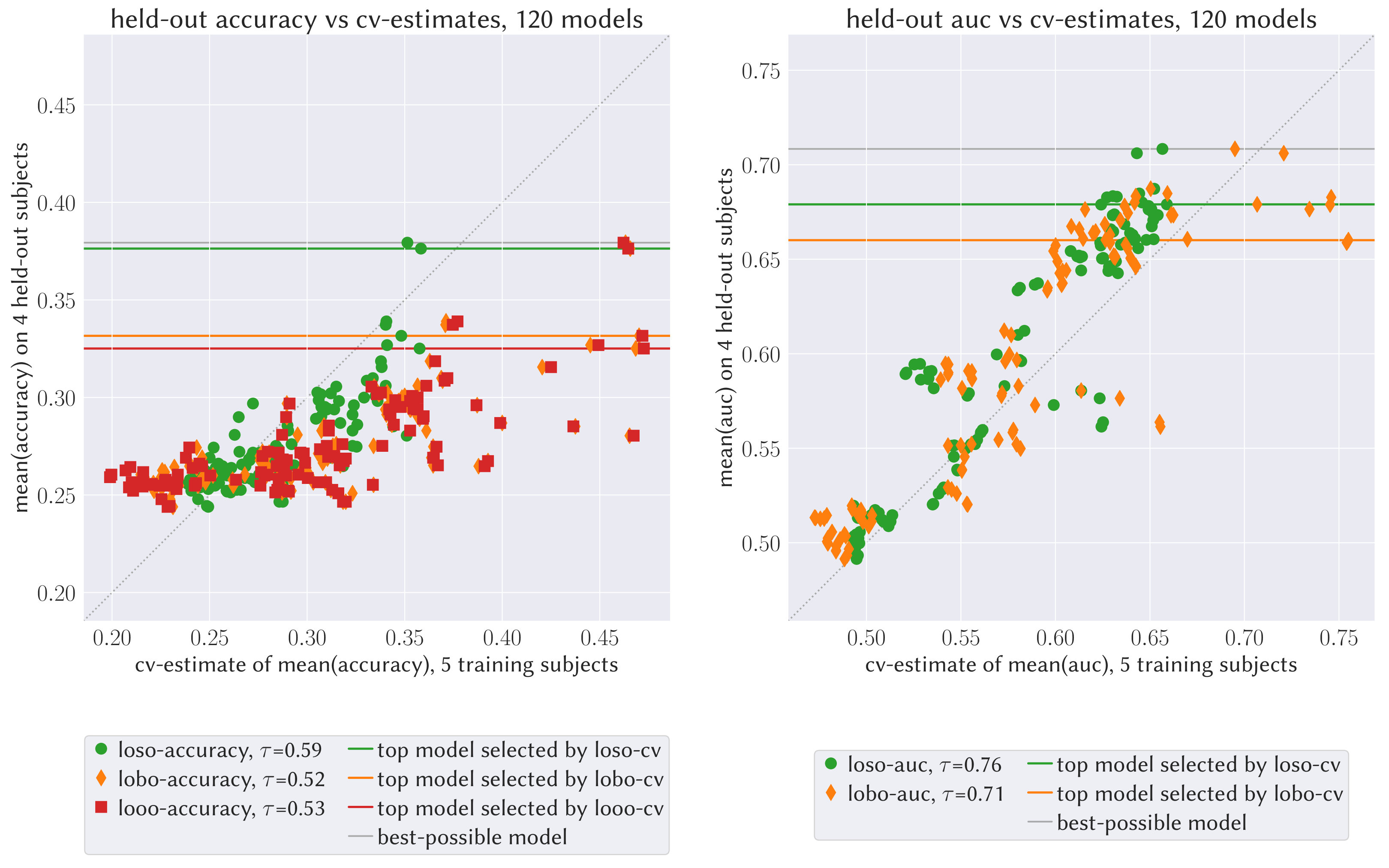
models were derived on the training data comprising recordings of the first subjects. Models relied on different sets of extracted timeseries components: the re-referenced EEG channels, different sets of PCA components with varying variance-explained ratios, and sets of coroICA components using neighbouring covariance pairs and a partition size of 15 seconds (cf. [80] for more details on coroICA). Signals were bandpass filtered in different frequency bands (, , , and ). For each trial and feature set, bandpower features for classification were obtained as the log-variance of the bandpass-filtered signal during seconds of each trial. For each of the configurations of trial features, we fitted different linear discriminant analysis classifiers without shrinkage, with automatic shrinkage based on the Ledoit-Wolf lemma, and shrinkage parameter settings , , and . These pipelines were fitted once on the entire training data and classification accuracies and areas under the receiver operating curve scores obtained on held-out subjects (-axes in Figure 3). Classifier performance was cross-validated on the training data following the following three different cross-validation schemes (cross-validation scores are shown on the -axes in Figure 3):
- loso-cv
-
Leave-one-subject-out cross-validation is the proposed cross-validation scheme. We hold out data corresponding to each training subject once, fit an LDA classifier on the remaining training data, and assess the models accuracy on the held-out training subject. The average of those cross-validation scores reflects how robustly each of the classifier models performs across environments (here subjects).
- lobo-cv
-
Leave-one-block-out cross-validation is a -fold cross-validation scheme that is similar to the above loso-cv scheme, where the training data is split into random blocks of roughly equal size. Not respecting the environment structure within the training data, this cross-validation scheme does not capture a models robustness across environments.
- looo-cv
-
Leave-one-observation-out cross-validation leaves out a single observation and is equivalent to lobo-cv with a block size of one.
In Figure 3 we display the results of the different cross-validation schemes and the Kendall’s rank correlation between the different cv-scores derived on the training data and a model’s classification performance on the four held-out subjects. The loso-cv scores correlate more strongly with held-out model performance and thereby slightly better resolve the relative model performance. Considering the held-out performance for the models with top cv-scores, we observe that selecting models based on the loso-cv score may indeed select models that tend to perform slightly better on new unseen subjects. Furthermore, comparing the displacement of the model scores from the diagonal shows that the loso-cv scheme’s estimates are less-biased than the lobo and looo cross-validation scores, when used as an estimate for the performance on held-out subjects; this is in line with [111].
4.3 Robustness and variable constructions
Whether distributional robustness holds can depend on whether we consider the right variables. This is shown by the following example. Assume that the target is caused by the two brain signals and via
for some , , and noise variable . Assume further that the environment influences the covariates and via and , but does not influence directly. Here, and may represent neuronal activity in two brain regions that are causal for reaction times while may indicate the time of day or respiratory activity. We then have the invariance property
If, however, we were to construct or—due to limited measurement ability—only be able to observe , then whenever we would find that
This conditional dependence is due to many value pairs for leading to the same value of : Given , the value of holds information about whether say or is more probable and thus–since and enter with different weights–holds information about ; and are conditionally dependent given . Thus, the invariance may break down when aggregating variables in an ill-suited way. This example is generic in that the same conclusions hold for all assignments and , as long as causal minimality, a weak form of faithfulness, is satisfied [100].
Rather than taking the lack of robustness as a deficiency, we believe that this observation has the potential to help us finding the right variables and granularity to model our system of interest. If we are given several environments, the guiding principle of distributional robustness can nudge our variable definition and ROI definition towards the construction of variables that are more suitable for causally modelling some cognitive function. If some ROI activity or some EEG bandpower feature does not satisfy any invariance across environments then we may conclude that our variable representation is misaligned with the underlying causal mechanisms or that important variables have not been observed (assuming that the environments do not act on directly).
This idea can be illustrated by a thought experiment that is a variation of the LDL-HDL example in Section 3.2: Assume we wish to aggregate multiple voxel-activities and represent them by the activity of a ROI defined by those voxels. For example, let us consider the reaction time scenario (Example A, Section 1.1) and voxels . Then we may aggregate the voxels to obtain a macro-level model in which we can still sensibly reason about the effect of an intervention on the treatment variable onto the distribution of , the ROIs average activity. Yet, the model is in general not causally consistent with the original model. First, our ROI may be chosen too coarse such that for with the interventional distributions induced by the micro-level model corresponding to setting all or alternatively to do not coincide—for example, a ROI that effectively captures the global average voxel-activity cannot resolve whether a higher activity is due to increased reaction-time-driving neuronal entities or due to some upregulation of other neuronal processes unrelated to the reaction time, such as respiratory activity. This ROI would be ill-suited for causal reasoning and non-robust as there are two micro-level interventions that imply different distributions on the reaction times while corresponding to the same intervention setting with in the macro-level model. Second, our ROI may be defined too fine grained such that, for example, the variable representation does only pick up on the left-hemisphere hub of a distributed neuronal process relevant for reaction times. If the neuronal process has different laterality in different subjects, then predicting the effects of interventions on only the left-hemispherical neuronal activity cannot be expected to translate to all subjects. Here, a macro-variable that averages more voxels, say symmetric of both hemispheres, may be more robust to reason about the causes of reaction times than the more fine grained unilateral ROI. In this sense, seeking for variable constructions that enable distributionally robust models across subjects, may nudge us to meaningful causal entities. The spatially refined and finer resolved cognitive atlas obtained by [112], whose map definition procedure was geared towards an atlas that would be robustness across multiple studies and different experimental conditions, may be seen as an indicative manifestation of the above reasoning.
4.4 Existing methods exploiting robustness
We now present some existing methods that explicitly consider the invariance of a model. While many of these methods are still in their infancy when considering real world applications, we believe that further development in that area could play a vital role when tackling causal questions in cognitive neuroscience.
Robust Independent Component Analysis.
Independent component analysis (ICA) is commonly performed in the analysis of magneto- and electro-electroencephalography (MEG and EEG) data in order to invert the inevitable measurement transformation that leaves us with observations of a linear superposition of underlying cortical (and non-cortical) activity. The basic ICA model assumes our vector of observed variables is being generated as where is a mixing matrix and is a vector of unobserved mutually independent source signals. The aim is to find the unmixing matrix . If we perform ICA on individual subjects’ data separately, the resulting unmixing matrices will often differ between subjects. This not only hampers the interpretation of the resulting sources as some cortical activity that we can identify across subjects, it also hints—in light of the above discussion—at some unexplained variation that is due to shifts in background conditions between subjects such as different cap positioning or neuroanatomical variation. Instead of simply pooling data across subjects, [80] propose a methodology that explicitly exploits the existence of environments, that is, the fact that EEG samples can be grouped by subjects they were recorded from. This way, the proposed confounding-robust ICA (coroICA) procedure identifies an unmixing of the signals that generalises to new subjects. The additional robustness resulted, for their considered example, in improved classification accuracies on held-out subjects and can be viewed as a first-order adjustment for subject specific differences. The application of ICA procedures to pooled data will generally result in components that do not robustly transfer to new subjects and are thus necessarily variables that do not lend themselves for a causal interpretation. The coroICA procedure aims to exploit the environments to identify unmixing matrices that generalise across subjects.
Causal discovery with exogenous variation.
Invariant causal prediction, proposed by [74], aims at identifying the parents of within a set of covariates . We have argued that the true causal model is invariant across environments, see Equation (2), if the data are obtained in different environments and the environment does not directly influence . That is, when enumerating all invariant models by searching through subsets of , one of these subsets must be the set of causal parents of . As a result, the intersection of all sets of covariates that yield invariant models is guaranteed to be a subset of the causes of . (Here, we define the intersection over the empty index set as the empty set.) Testing invariance with a hypothesis test to the level , say , one obtains that is contained in the set of parents of with high probability
Under faithfulness, the method can be shown to be robust against violation of the above assumptions. If the environment acts on directly, for example, there is no invariant set and in the presence of hidden variables, the intersection of invariant models can still be shown to be a subset of the ancestors of with large probability.
It is further possible to model the environment as a random variable (using an indicator variable, for example), that is often called a context variable. One can then exploit the background knowledge of its exogeneity to identify the full causal structure instead of focussing on identifying the causes of a target variable. Several approaches have been suggested [[, for example,]]Spirtes2000, Eaton2007, Zhang-ijcai2017, Mooij++_JMLR_20. Often, these methods first identify the target of the intervention and then exploit known techniques of constraint- or score-based methods. Some of the above methods also make use of time as a context variable or environment [125, 79].
Anchor regression.
We argued above that focusing on invariance has an advantage when inferring causal structure from data. If we are looking for generalisability across environments, however, focusing solely on invariance may be too restrictive. Instead, we may select the most predictive model among all invariant models. The idea of anchor regression is to explicitly trade off invariance and predictability [87]. For a target variable , predictor variables , and so-called anchor variables that represent the different environments and are normalised to have unit variance, the anchor regression coefficients are obtained as solutions to the following minimisation problem
Higher parameters steer the regression towards more invariant predictions (converging against the two stage least squares solutions in identifiable instrumental variable settings). For we recover the ordinary least square solution. The solution can be shown to have the best predictive power under shift interventions up to a certain strength that depends on . As before, the anchor variables can code time, environments, subjects, or other factors, and we thus obtain a regression that is distributionally robust against shifts in those factors.
4.5 Time series data
So far, we have mainly focused on the setting of i.i.d. data. Most of the causal inference literature dealing with time dependency considers discrete-time models. This comes with additional complications for causal inference. For example, there are ongoing efforts to adapt causal inference algorithms and account for sub- or sup-sampling and temporal aggregation [23, 46]. Problems of temporal aggregation relate to Challenge 2 of finding the right variables, which is a conceptual problem in time series models that requires us to clarify our notion of intervention for time-evolving systems [88]. When we observe time series with non-stationarities we may consider these as resulting from some unknown shift interventions. That is, non-stationarities over time may be due to shifts in the background conditions and as such can be understood as shifts in environments analogous to the i.i.d. setting. This way, we may again leverage the idea of distributional robustness for inference on time-evolving systems for which targeted interventional data is scarce. Extensions of invariant causal prediction to time series data that aim to leverage such variation have been proposed by [20, 79] and the ICA procedure described in Section 4.4 also exploits non-stationarity over time. SCMs extend to continuous-time models [72], where the idea to trade off prediction and invariance has been applied to the problem of inferring chemical reaction networks [78].
A remark is in order if we wish to describe time-evolving systems by one causal summary graph where each time series component is collapsed into one node: For this to be reasonable, we need to assume a time-homogeneous causal structure. Furthermore, it requires us to carefully clarify its causal semantics: While summary graphs can capture the existence of cause-effect relationships, they do in general not correspond to a structural causal model that admits a causal semantics nor enables interventional predictions that are consistent with the underlying time-resolved structural causal model [88, 49]. That is, the wrong choice of time-agnostic variables and corresponding interventions may be ill-suited to represent the cause-effect relationships of a time-evolving system [[, cf. Challenge 2 and]]rubenstein2017causal,janzing2018structural.
5 Conclusion and future work
Causal inference in cognitive neuroscience is ambitious. It is important to continue the open discourse about the many challenges, some of which are mentioned above. Thanks to the open and critical discourse there is great awareness and caution when interpreting neural correlates [84]. Yet, “FC [functional connectivity] researchers already work within a causal inference framework, whether they realise it or not” [86].
In this article we have provided our view on the numerous obstacles to a causal understanding of cognitive function. If we, explicitly or often implicitly, ask causal questions, we need to employ causal assumptions and methodology. We propose to exploit that causal models using the right variables are distributionally robust. In particular, we advocate distributional robustness as a guiding principle for causality in cognitive neuroscience. While causal inference in general and in cognitive neuroscience in particular is a challenging task, we can at least exploit the rational to refute models and variables as non-causal that are frail to shifts in the environment. This guiding principle does not necessarily identify causal variables nor causal models, but it nudges our search into the right direction away from frail models and non-causal variables. While we presented first attempts that aim to leverage observations obtained in different environments (cf. Section 4.4), this article poses more questions for future research than it answers.
We believe that procedures that exploit environments during training are a promising avenue for future research. While we saw mildly positive results in our case study, further research needs to show whether this trend persists in studies with many subjects. It may be possible to obtain improvements when combining predictive scores on held-out-subjects with other measures of invariance and robustness. The development of such methods may be spurred and guided by field-specific benchmarks (or competitions) that assess models’ distributional robustness across a wide range of scenarios, environments, cognitive tasks, and subjects.
When considering robustness or invariance across trainings environments, the question arises how the ability to infer causal structure and the generalisation performance to unseen environments depend on the number of training environments. While first attempts have been made to theoretically understand that relation [87, 21], most of the underlying questions are still open. We believe that an answer would depend on the strength of the interventions, the sample size, the complexity of the model class and, possibly, properties of the (meta-)distribution of environments.
We believe that advancements regarding the errors-in-variable problem may have important implications for cognitive neuroscience. Nowadays, we can obtain neuroimaging measurements at various spatial and temporal resolutions using, among others, fMRI, MEG and EEG, positron emission tomography, or near-infrared spectroscopy [31, 81]. Yet, all measurement modalities are imperfect and come with different complications. One general problem is that the observations are corrupted by measurement noise. The errors-in-variables problem complicates even classical regression techniques where we wish to model but only have access to observations of a noise-corrupted [92]. This inevitably carries over and hurdles causal inference as the measurement noise spoils conditional independence testing, biases any involved regression steps, and troubles additive noise approaches that aim to exploit noise properties for directing causal edges and methods testing for invariance. First steps addressing these issues in the context of causal discovery have been proposed by [124, 8, 91].
Summarising, we believe that there is a need for causal models if we aim to understand the neuronal underpinnings of cognitive function. Only causal models equip us with concepts that allow us to explain, describe, predict, manipulate, deal and interact with, and reason about a system and that allow us to generalise to new, unseen environments. A merely associational model suffices to predict naturally unfolding disease progression, for example. We need to obtain understanding in form of a causal model if our goal is to guide rehabilitation after cognitive impairment or to inform the development of personalised drugs that target specific neuronal populations. Distributional robustness and generalisability to unseen environments is an ambitious goal, in particular in biological systems and even more so in complex systems such as the human brain. Yet, it may be the only and most promising way forward.
Acknowledgments
The authors thank the anonymous reviewers for their constructive and helpful feedback on an earlier version of this manuscript. SW was supported by the Carlsberg Foundation.
References
- [1] J. Aldrich “Autonomy” In Oxford Economic Papers 41, 1989, pp. 15–34
- [2] Andrea Antal and Christoph S Herrmann “Transcranial alternating current and random noise stimulation: possible mechanisms” In Neural Plasticity 2016 Hindawi, 2016
- [3] Dominik R Bach, Mkael Symmonds, Gareth Barnes and Raymond J Dolan “Whole-Brain Neural Dynamics of Probabilistic Reward Prediction” In Journal of Neuroscience 37.14, 2017, pp. 3789–3798
- [4] Sander Beckers, Frederick Eberhardt and Joseph Y Halpern “Approximate Causal Abstraction” In Proceedings of the Thirty-Fifth Conference on Uncertainty in Artificial Intelligence (UAI) AUAI Press, 2019
- [5] Sander Beckers and Joseph Y Halpern “Abstracting Causal Models” In Proceedings of the Thirty-Third AAAI Conference on Artificial Intelligence AAAI Press, 2019
- [6] Til Ole Bergmann and Gesa Hartwigsen “Inferring Causality from Noninvasive Brain Stimulation in Cognitive Neuroscience” Forthcoming In Journal of Cognitive Neuroscience, 2020, pp. 1–29
- [7] Sven Bestmann and Vincent Walsh “Transcranial electrical stimulation” In Current Biology 27.23 Elsevier, 2017, pp. R1258–R1262
- [8] T. Blom, A. Klimovskaia, S. Magliacane and J.. Mooij “An Upper Bound for Random Measurement Error in Causal Discovery” In Proceedings of the 34th Annual Conference on Uncertainty in Artificial Intelligence (UAI), 2018
- [9] Kenneth A Bollen “Structural Equations with Latent Variables” John Wiley & Sons, 1989
- [10] Stephan Bongers, Jonas Peters, Bernhard Schölkopf and Joris M Mooij “Theoretical Aspects of Cyclic Structural Causal Models” In arXiv preprint arXiv:1611.06221, 2018
- [11] Michael Breakspear “Dynamic and stochastic models of neuroimaging data: A comment on Lohmann et al.” In NeuroImage 75, 2013, pp. 270–274
- [12] P. Bühlmann, J. Peters and J. Ernest “CAM: Causal Additive Models, high-dimensional order search and penalized regression” In Annals of Statistics 42, 2014, pp. 2526–2556
- [13] N. Cartwright “Two Theorems on Invariance and Causality” In Philosophy of Science 70.1, 2003, pp. 203–224
- [14] N. Cartwright “Causality, invariance and policy” In The Oxford handbook of philosophy of economics New York, NY: Oxford University Press, 2009, pp. 410–423
- [15] Krzysztof Chalupka, Frederick Eberhardt and Pietro Perona “Multi-Level Cause-Effect Systems” In Proceedings of the 19th International Conference on Artificial Intelligence and Statistics 51, Proceedings of Machine Learning Research PMLR, 2016, pp. 361–369
- [16] Krzysztof Chalupka, Pietro Perona and Frederick Eberhardt “Visual Causal Feature Learning” In Proceedings of the Thirty-First Conference on Uncertainty in Artificial Intelligence (UAI) AUAI Press, 2015
- [17] Daniel Chicharro and Stefano Panzeri “Algorithms of causal inference for the analysis of effective connectivity among brain regions” In Frontiers in Neuroinformatics 8, 2014, pp. 64
- [18] D.. Chickering “Optimal structure identification with greedy search” In Journal of Machine Learning Research 3, 2002, pp. 507–554
- [19] G.. Chow “Tests of equality between sets of coefficients in two linear regressions” In Econometrica 28, 1960, pp. 591–605
- [20] R. Christiansen and J. Peters “Invariant Causal Prediction in the Presence of Latent Variables” In arXiv preprint arXiv:1808.05541, 2018
- [21] R. Christiansen et al. “The Difficult Task of Distribution Generalization in Nonlinear Models” In arXiv preprint arXiv:2006.07433, 2020
- [22] Denis Conniffe “R.A. Fisher and the development of statistics - a view in his centerary year” In Journal of the Statistical and Social Inquiry Society of Ireland 26.3, 1991, pp. 55–108
- [23] David Danks and Sergey Plis “Learning causal structure from undersampled time series” Carnegie Mellon University, 2013
- [24] G. Darmois “Analyse générale des liaisons stochastiques” In Revue de l’Institut International de Statistique 21, 1953, pp. 2–8
- [25] Tyler Davis et al. “What do differences between multi-voxel and univariate analysis mean? How subject-, voxel-, and trial-level variance impact fMRI analysis” In NeuroImage 97, 2014, pp. 271–283
- [26] Julien Dubois et al. “Causal mapping of emotion networks in the human brain: Framework and initial findings” In Neuropsychologia, 2017
- [27] D. Eaton and K.. Murphy “Exact Bayesian structure learning from uncertain interventions” In Proceedings of the 11th International Conference on Artificial Intelligence and Statistics (AISTATS), 2007, pp. 107–114
- [28] Frederick Eberhardt “Experimental indistinguishability of causal structures” In Philosophy of Science 80.5 University of Chicago Press, 2013, pp. 684–696
- [29] Frederick Eberhardt “Green and grue causal variables” In Synthese 193.4, 2016, pp. 1029–1046
- [30] Gaute T Einevoll, Christoph Kayser, Nikos K Logothetis and Stefano Panzeri “Modelling and analysis of local field potentials for studying the function of cortical circuits” In Nature Reviews Neuroscience 14.11 Nature Publishing Group, 2013, pp. 770–785
- [31] Aaron Filler “The history, development and impact of computed imaging in neurological diagnosis and neurosurgery: CT, MRI, and DTI” In Nature Precedings Nature Publishing Group, 2009
- [32] K.. Friston, L. Harrison and W. Penny “Dynamic causal modelling” In NeuroImage 19.4, 2003, pp. 1273–1302
- [33] Karl Friston, Jean Daunizeau and Klaas Enno Stephan “Model selection and gobbledygook: Response to Lohmann et al.” In NeuroImage 75, 2013, pp. 275–278
- [34] C… Granger “Investigating Causal Relations by Econometric Models and Cross-spectral Methods” In Econometrica 37.3, 1969, pp. 424–438
- [35] Moritz Grosse-Wentrup, Dominik Janzing, Markus Siegel and Bernhard Schölkopf “Identification of causal relations in neuroimaging data with latent confounders: An instrumental variable approach” In NeuroImage 125, 2016, pp. 825–833
- [36] L. Györfi, M. Kohler, A. Krzyżak and H. Walk “A Distribution-Free Theory of Nonparametric Regression” Springer, 2002
- [37] T. Haavelmo “The Probability Approach in Econometrics” In Econometrica 12, 1944, pp. S1–S115 (supplement)
- [38] S. Haufe et al. “On the interpretation of weight vectors of linear models in multivariate neuroimaging” In NeuroImage 87, 2014, pp. 96–110
- [39] Suzana Herculano-Houzel “The remarkable, yet not extraordinary, human brain as a scaled-up primate brain and its associated cost” In Proceedings of the National Academy of Sciences 109.Supplement 1 National Academy of Sciences, 2012, pp. 10661–10668
- [40] Christoph S Herrmann, Stefan Rach, Toralf Neuling and Daniel Strüber “Transcranial alternating current stimulation: a review of the underlying mechanisms and modulation of cognitive processes” In Frontiers in human neuroscience 7 Frontiers, 2013, pp. 279
- [41] Erik P. Hoel “When the Map Is Better Than the Territory” In Entropy 19.5, 2017
- [42] Erik P Hoel, Larissa Albantakis and Giulio Tononi “Quantifying causal emergence shows that macro can beat micro” In Proceedings of the National Academy of Sciences 110.49, 2013, pp. 19790–19795
- [43] K.. Hoover “Causality in Economics and Econometrics” In The New Palgrave Dictionary of Economics Basingstoke, UK: Palgrave Macmillan, 2008
- [44] Patrik O Hoyer et al. “Nonlinear causal discovery with additive noise models” In Advances in Neural Information Processing Systems 21 (NeurIPS) NeurIPS Foundation, 2008, pp. 689–696
- [45] Alexander G Huth et al. “Decoding the Semantic Content of Natural Movies from Human Brain Activity” In Frontiers in Systems Neuroscience 10, 2016, pp. 81
- [46] Antti Hyttinen et al. “Causal discovery from subsampled time series data by constraint optimization” In Proceedings of the Eighth International Conference on Probabilistic Graphical Models 52, Proceedings of Machine Learning Research PMLR, 2016, pp. 216–227
- [47] G.. Imbens and D.. Rubin “Causal Inference for Statistics, Social, and Biomedical Sciences” Cambridge University Press, 2015
- [48] Fattaneh Jabbari, Joseph Ramsey, Peter Spirtes and Gregory Cooper “Discovery of causal models that contain latent variables through Bayesian scoring of independence constraints” In Joint European Conference on Machine Learning and Knowledge Discovery in Databases, 2017, pp. 142–157 Springer
- [49] Dominik Janzing, Paul Rubenstein and Bernhard Schölkopf “Structural causal models for macro-variables in time-series” In arXiv preprint arXiv:1804.03911, 2018
- [50] Kohitij Kar, Takuya Ito, Michael W. Cole and Bart Krekelberg “Transcranial alternating current stimulation attenuates BOLD adaptation and increases functional connectivity” In Journal of Neurophysiology 123.1, 2020, pp. 428–438
- [51] S. Lauritzen “Graphical Models” Oxford University Press, 1996
- [52] S.. Lauritzen, A.. Dawid, B.. Larsen and H.-G. Leimer “Independence properties of directed markov fields” In Networks 20, 1990, pp. 491–505
- [53] Jin Hyung Lee et al. “Global and local fMRI signals driven by neurons defined optogenetically by type and wiring” In Nature 465.7299 Nature Publishing Group, 2010, pp. 788–792
- [54] Zhifeng Liang et al. “Mapping the functional network of medial prefrontal cortex by combining optogenetics and fMRI in awake rats” In NeuroImage 117, 2015, pp. 114–123
- [55] Nikos K Logothetis “What we can do and what we cannot do with fMRI” In Nature 453.7197 Nature Publishing Group, 2008, pp. 869–878
- [56] Gabriele Lohmann, Kerstin Erfurth, Karsten Müller and Robert Turner “Critical comments on dynamic causal modelling” In NeuroImage 59.3, 2012, pp. 2322–2329
- [57] Gabriele Lohmann, Karsten Müller and Robert Turner “Response to commentaries on our paper: Critical comments on dynamic causal modelling” In NeuroImage 75, 2013, pp. 279–281
- [58] Virginia López-Alonso, Binith Cheeran, Dan Rio-Rodriguez and Miguel Fernández-del-Olmo “Inter-individual variability in response to non-invasive brain stimulation paradigms” In Brain stimulation 7.3 Elsevier, 2014, pp. 372–380
- [59] R. Lucas “Econometric policy evaluation: A critique” In Carnegie-Rochester Conference Series on Public Policy 1.1, 1976, pp. 19–46
- [60] I. M. and D. Lopez-Paz “Invariant Risk Minimization” In arXiv preprint arXiv:1907.02893, 2019
- [61] D. Marinazzo, M. Pellicoro and S. Stramaglia “Kernel-Granger causality and the analysis of dynamical networks” In Physical Review E 77.5 American Physical Society, 2008, pp. 056215
- [62] Daniele Marinazzo, Wei Liao, Huafu Chen and Sebastiano Stramaglia “Nonlinear connectivity by Granger causality” In NeuroImage 58.2, 2011, pp. 330–338
- [63] A Mastakouri, B Schölkopf and D Janzing “Selecting causal brain features with a single conditional independence test per feature” In Advances in Neural Information Processing Systems 32 (NeurIPS) NeurIPS Foundation, 2019, pp. 12532–12543
- [64] Helen S Mayberg et al. “Deep Brain Stimulation for Treatment-Resistant Depression” In Neuron 45.5 Elsevier, 2005, pp. 651–660
- [65] David Marc Anton Mehler and Konrad Paul Kording “The lure of causal statements: Rampant mis-inference of causality in estimated connectivity” In arXiv preprint arXiv:1812.03363, 2018
- [66] Ravi D Mill, Takuya Ito and Michael W Cole “From connectome to cognition: The search for mechanism in human functional brain networks” In NeuroImage 160 Elsevier, 2017, pp. 124–139
- [67] J.. Mooij, S. Magliacane and T. Claassen “Joint Causal Inference from Multiple Contexts” In Journal of Machine Learning Research 21.99, 2020, pp. 1–108
- [68] Jeanette A Mumford and Joseph D Ramsey “Bayesian networks for fMRI: A primer” In NeuroImage 86, 2014, pp. 573–582
- [69] Michael A. Nitsche et al. “Transcranial direct current stimulation: State of the art 2008” In Brain Stimulation 1.3, 2008, pp. 206–223
- [70] P.. Nunez and R. Srinivasan “Electric Fields of the Brain” Oxford University Press, 2006
- [71] Judea Pearl “Causality” Cambridge University Press, 2009
- [72] J. Peters, S. Bauer and N. Pfister “Causal models for dynamical systems” In arXiv preprint arXiv:2001.06208, 2020
- [73] J. Peters and P. Bühlmann “Identifiability of Gaussian Structural Equation Models with Equal Error Variances” In Biometrika 101.1, 2014, pp. 219–228
- [74] J. Peters, P. Bühlmann and N. Meinshausen “Causal inference using invariant prediction: identification and confidence intervals” In Journal of the Royal Statistical Society: Series B (with discussion) 78.5, 2016, pp. 947–1012
- [75] J. Peters, D. Janzing and B. Schölkopf “Causal Inference on Time Series using Structural Equation Models” In Advances in Neural Information Processing Systems 26 (NeurIPS) NeurIPS Foundation, 2013, pp. 585–592
- [76] J. Peters, D. Janzing and B. Schölkopf “Elements of Causal Inference” MIT Press, 2017
- [77] J. Peters, J.. Mooij, D. Janzing and B. Schölkopf “Causal Discovery with Continuous Additive Noise Models” In Journal of Machine Learning Research 15, 2014, pp. 2009–2053
- [78] N. Pfister, S. Bauer and J. Peters “Learning stable and predictive structures in kinetic systems” In Proceedings of the National Academy of Sciences 116.51 National Academy of Sciences, 2019, pp. 25405–25411
- [79] N. Pfister, P. Bühlmann and J. Peters “Invariant Causal Prediction for Sequential Data” In Journal of the American Statistical Association 114.527, 2018, pp. 1264–1276
- [80] Niklas Pfister, Sebastian Weichwald, Peter Bühlmann and Bernhard Schölkopf “Robustifying Independent Component Analysis by Adjusting for Group-Wise Stationary Noise” In Journal of Machine Learning Research 20.147, 2019, pp. 1–50
- [81] Russell A Poldrack “The new mind readers: What neuroimaging can and cannot reveal about our thoughts” Princeton University Press, 2018
- [82] Jonathan D Power et al. “Functional network organization of the human brain” In Neuron 72.4 Elsevier, 2011, pp. 665–678
- [83] J D Ramsey et al. “Six problems for causal inference from fMRI” In NeuroImage 49.2, 2010, pp. 1545–1558
- [84] Geraint Rees, Gabriel Kreiman and Christof Koch “Neural correlates of consciousness in humans” In Nature Reviews Neuroscience 3, 2002, pp. 261–270
- [85] H. Reichenbach “The Direction of Time” University of California Press, 1956
- [86] Andrew T Reid et al. “Advancing functional connectivity research from association to causation” In Nature neuroscience 1.10 Nature Publishing Group, 2019
- [87] Dominik Rothenhäusler, Nicolai Meinshausen, Peter Bühlmann and Jonas Peters “Anchor regression: heterogeneous data meets causality” In arXiv preprint arXiv:1801.06229, 2018
- [88] Paul K Rubenstein et al. “Causal Consistency of Structural Equation Models” In Proceedings of the Thirty-Third Conference on Uncertainty in Artificial Intelligence (UAI), 2017
- [89] Ruben Sanchez-Romero and Michael W Cole “Combining Multiple Functional Connectivity Methods to Improve Causal Inferences” Forthcoming In Journal of Cognitive Neuroscience, 2020, pp. 1–15
- [90] Ruben Sanchez-Romero et al. “Estimating feedforward and feedback effective connections from fMRI time series: Assessments of statistical methods” In Network Neuroscience 3.2, 2019, pp. 274–306
- [91] R. Scheines and J. Ramsey “Measurement error and causal discovery” In CEUR Workshop Proceedings 1792, 2016, pp. 1–7
- [92] Susanne M Schennach “Recent advances in the measurement error literature” In Annual Review of Economics 8 Annual Reviews, 2016, pp. 341–377
- [93] B. Schölkopf et al. “On causal and anticausal learning” In Proceedings of the 29th International Conference on Machine Learning (ICML) Omnipress, 2012, pp. 1255–1262
- [94] R. Shah and J. Peters “The Hardness of Conditional Independence Testing and the Generalised Covariance Measure” In Annals of Statistics (accepted), ArXiv e-prints (1804.07203), 2020
- [95] S. Shimizu, P.. Hoyer, A. Hyvärinen and A. Kerminen “A Linear Non-Gaussian Acyclic model for Causal Discovery” In Journal of Machine Learning Research 7.10, 2006, pp. 2003–2030
- [96] Ricardo Silva, Richard Scheine, Clark Glymour and Peter Spirtes “Learning the structure of linear latent variable models” In Journal of Machine Learning Research 7, 2006, pp. 191–246
- [97] V.. Skitovič “Linear combinations of independent random variables and the normal distribution law” In Selected Translations in Mathematical Statistics and Probability 2, 1962, pp. 211–228
- [98] Stephen M Smith “The future of FMRI connectivity” In Neuroimage 62.2 Elsevier, 2012, pp. 1257–1266
- [99] Stephen M Smith et al. “Network modelling methods for FMRI” In Neuroimage 54.2 Elsevier, 2011, pp. 875–891
- [100] Peter Spirtes, Clark N Glymour and Richard Scheines “Causation, Prediction, and Search” MIT Press, 2001
- [101] Peter Spirtes and Richard Scheines “Causal Inference of Ambiguous Manipulations” In Philosophy of Science 71.5, 2004, pp. 833–845
- [102] Daniel Steinberg “The Cholesterol Wars” Academic Press, 2007
- [103] S. Stramaglia, Guo-Rong Wu, M. Pellicoro and D. Marinazzo “Expanding the transfer entropy to identify information circuits in complex systems” In Physical Review E 86.6 American Physical Society, 2012, pp. 066211
- [104] Sebastiano Stramaglia, Jesus M Cortes and Daniele Marinazzo “Synergy and redundancy in the Granger causal analysis of dynamical networks” In New Journal of Physics 16.10 IOP Publishing, 2014, pp. 105003
- [105] M. Tangermann et al. “Review of the BCI Competition IV” In Frontiers in Neuroscience 6, 2012, pp. 55
- [106] Michael T Todd, Leigh E Nystrom and Jonathan D Cohen “Confounds in multivariate pattern analysis: Theory and rule representation case study” In NeuroImage 77, 2013, pp. 157–165
- [107] A Stewart Truswell “Cholesterol and Beyond” Springer, 2010
- [108] Lucina Q. Uddin, B.. Yeo and R. Spreng “Towards a Universal Taxonomy of Macro-scale Functional Human Brain Networks” In Brain Topography 32.6, 2019, pp. 926–942
- [109] C. Uhler, G. Raskutti, P. Bühlmann and B. Yu “Geometry of the faithfulness assumption in causal inference” In Annals of Statistics 41.2, 2013, pp. 436–463
- [110] Pedro A Valdes-Sosa, Alard Roebroeck, Jean Daunizeau and Karl Friston “Effective connectivity: influence, causality and biophysical modeling” In Neuroimage 58.2 Elsevier, 2011, pp. 339–361
- [111] Gaël Varoquaux et al. “Assessing and tuning brain decoders: Cross-validation, caveats, and guidelines” Individual Subject Prediction In NeuroImage 145, 2017, pp. 166–179
- [112] Gaël Varoquaux et al. “Atlases of cognition with large-scale human brain mapping” In PLOS Computational Biology 14.11, 2018, pp. 1–18
- [113] Thomas Verma and Judea Pearl “Equivalence and Synthesis of Causal Models” In Proceedings of the Sixth Annual Conference on Uncertainty in Artificial Intelligence (UAI), 1990
- [114] Johannes Vosskuhl, Daniel Strüber and Christoph S Herrmann “Non-invasive brain stimulation: a paradigm shift in understanding brain oscillations” In Frontiers in human neuroscience 12 Frontiers, 2018, pp. 211
- [115] Lourens Waldorp, Ingrid Christoffels and Vincent Ven “Effective connectivity of fMRI data using ancestral graph theory: Dealing with missing regions” In NeuroImage 54.4, 2011, pp. 2695–2705
- [116] Sebastian Weichwald “Pragmatism and Variable Transformations in Causal Modelling”, 2019
- [117] Sebastian Weichwald, Arthur Gretton, Bernhard Schölkopf and Moritz Grosse-Wentrup “Recovery of non-linear cause-effect relationships from linearly mixed neuroimaging data” In Pattern Recognition in Neuroimaging (PRNI), 2016 International Workshop on, 2016 IEEE
- [118] Sebastian Weichwald, Moritz Grosse-Wentrup and Arthur Gretton “MERLiN: Mixture Effect Recovery in Linear Networks” In IEEE Journal of Selected Topics in Signal Processing 10.7, 2016, pp. 1254–1266
- [119] Sebastian Weichwald et al. “Causal interpretation rules for encoding and decoding models in neuroimaging” In NeuroImage 110, 2015, pp. 48–59
- [120] Sebastian Weichwald, Bernhard Schölkopf, Tonio Ball and Moritz Grosse-Wentrup “Causal and anti-causal learning in pattern recognition for neuroimaging” In Pattern Recognition in Neuroimaging (PRNI), 2014 International Workshop on, 2014 IEEE
- [121] James Woodward “Making Things Happen: A Theory of Causal Explanation” Oxford University Press, 2005
- [122] Alex Woolgar, Polina Golland and Stefan Bode “Coping with confounds in multivoxel pattern analysis: What should we do about reaction time differences? A comment on Todd, Nystrom & Cohen 2013” In NeuroImage 98, 2014, pp. 506–512
- [123] B.. Yeo et al. “The organization of the human cerebral cortex estimated by intrinsic functional connectivity” In Journal of Neurophysiology 106.3, 2011, pp. 1125–1165
- [124] K. Zhang et al. “Causal Discovery with Linear Non-Gaussian Models underMeasurement Error: Structural Identifiability Results” In Proceedings of the 34th Annual Conference on Uncertainty in Artificial Intelligence (UAI) AUAI Press, 2018
- [125] K. Zhang et al. “Causal Discovery from Nonstationary/Heterogeneous Data: Skeleton Estimation and Orientation Determination” In Proceedings of the 26th International Joint Conference on Artificial Intelligence (IJCAI), 2017, pp. 1347–1353
- [126] K. Zhang and A. Hyvärinen “On the Identifiability of the Post-Nonlinear Causal Model” In Proceedings of the Twenty-Fifth Annual Conference on Uncertainty in Artificial Intelligence (UAI) AUAI Press, 2009
- [127] Xun Zheng et al. “Learning sparse nonparametric DAGs” (to appear) In Proceedings of the 23rd International Conference on Artificial Intelligence and Statistics, 2020