ccc-Autoevolutes
Abstract
ccc-Autoevolutes are closed constant curvature space curves which are their own evolutes. A modified Frenet equation produces curves which are congruent to their evolutes. Using symmetries we construct closed curves by solving 2-parameter problems numerically. The images are made with the program 3D-XplorMath [2].
Classification: 53A04
Osculating circles moving along the curve can be seen in [3].
This paper is a continuation of [1]. It started with the challenge from Ekkehard-H. Tjaden to look for constant curvature curves which are congruent to their evolutes. The details are joint work.
Assume that the curve is parametrized by arc length , has constant curvature and its Frenet frame is . Its evolute is
| (1) | ||||
| (2) |
The velocity of the evolute is therefore
| (3) |
with
| (4) | ||||
| (5) | ||||
| (6) |
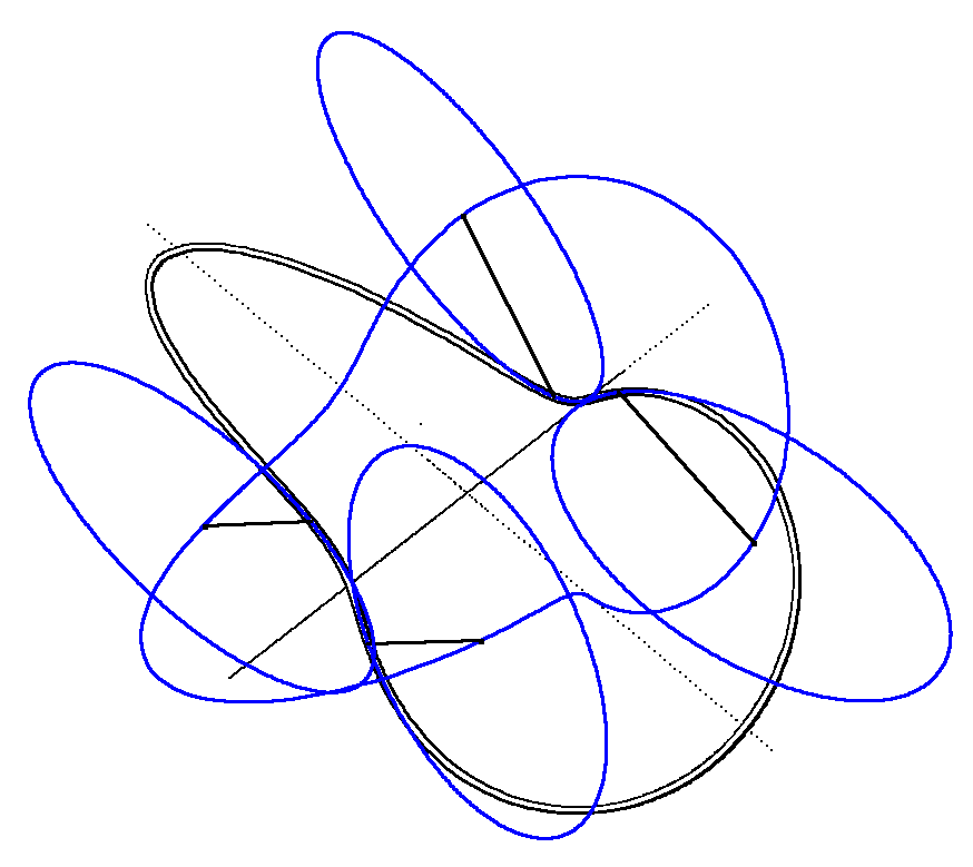
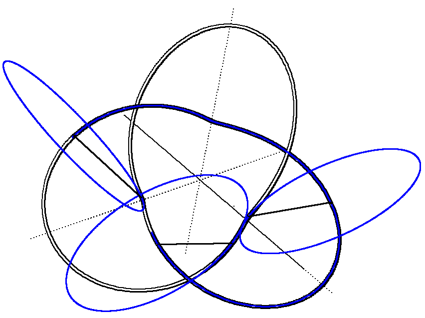
The two curves , are geodesics on the canal surface which envelops the spheres of radius with midpoints on the curve , because their principle normals , are orthogonal to the canal surface. This canal surface is, in the case of the two examples above, a wobbly torus – maybe that helps the visualization.
Constant curvature curves in general do not have congruent evolutes and even if , are congruent, this is difficult to check in case is parametrized by arc length. One may look for curves with non-constant velocity , choose in terms of and try to arrange things so that the first half of the curve is congruent to the evolute of the second half and vice versa. As a consequence both halves of the middle curve are congruent.This is achieved by the following version of the Frenet equations which Ekkehard suggested. It assumes and .
| (11) | ||||
| (12) | ||||
| (13) |
For our computations we choose first
and then
or also
.
We find it convenient not to restrict us to
, but to also vary the curvature.
Comparison with the standard Frenet equations shows
.
Note that
and
are, relative to
,
even functions. This implies that the principle normals at these
points are symmetry normals, saying that
rotations around these normals map the curve onto itself.
Closed
examples can therefore be found by solving the following 2-parameter problem:
a) get the symmetry normals to lie in a plane – they then automatically
all intersect in one point.
b) get neighbouring symmetry lines to intersect with
a rational angle – preferably angles like
, , ….
This looks similar to the case of single constant curvature curves. However in that case the constant Fourier term of the torsion is a parameter that allows to solve problem a) for all choices of other parameters. This allows to deal with problem b) assuming that a) is already solved. For the autoevolutes we have not found such a simplifying parameter. By trial and error one has to roughly close the curve. Only then does the automatic solution of the 2-paramter problem work and produce a high accuracy solution.
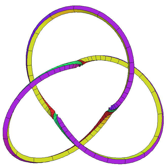
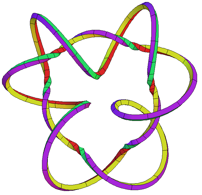
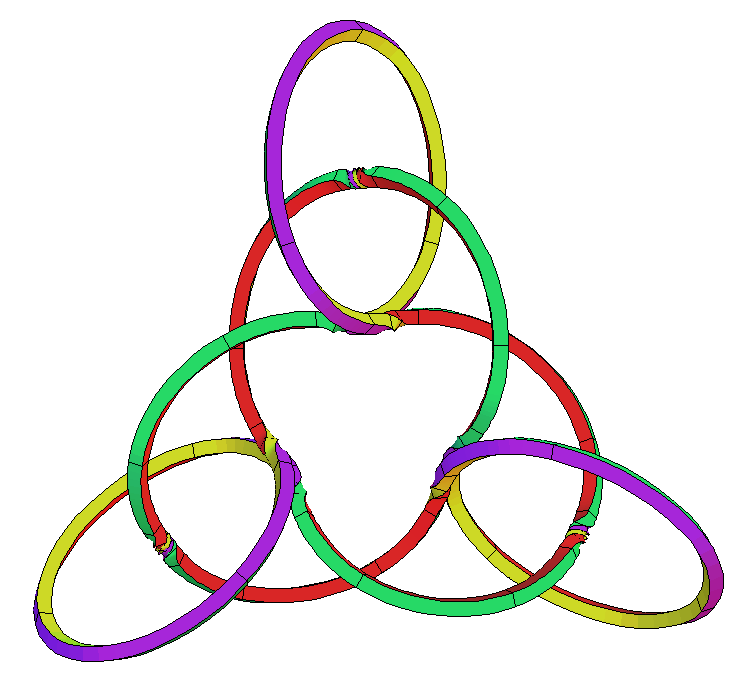
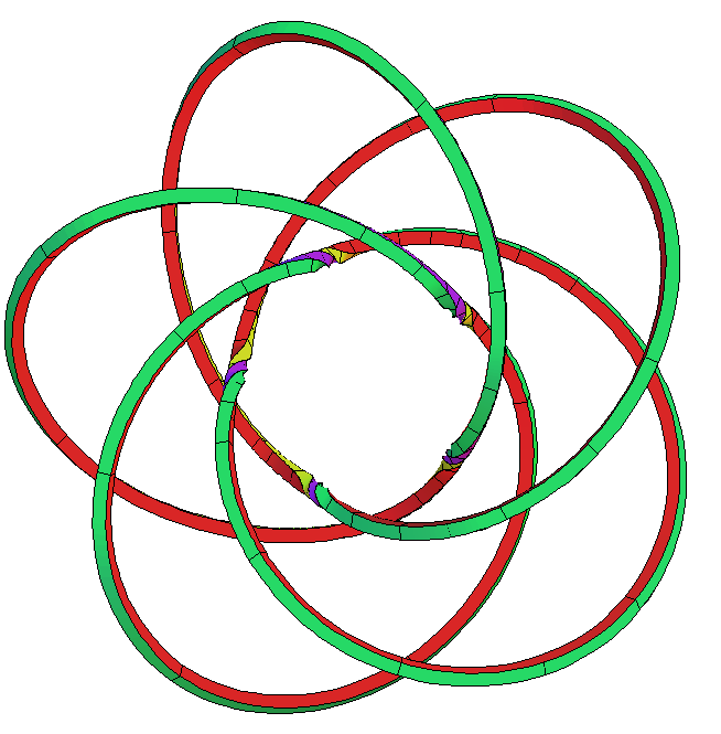
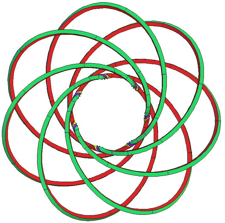
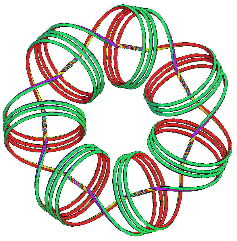
Note that we are using only three parameters to get these examples. If we change in sufficiently small steps then we can adjust to deform the examples as closed curves. Of course, if we add more (small) Fourier terms to the definition of , then we get higher dimensional deformation families. By changing the parameters without adjustment we get to the vicinity of other examples, which then are caught with our 2-dim equation solver. We found for odd and even autoevolutes which are -torus knots. We found them with additional inward loops as the second example above. The right example is still recognizable with , but for larger our examples are too complicated to print. Here are some examples:
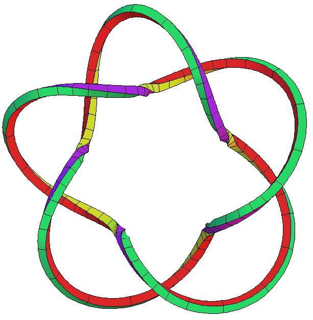
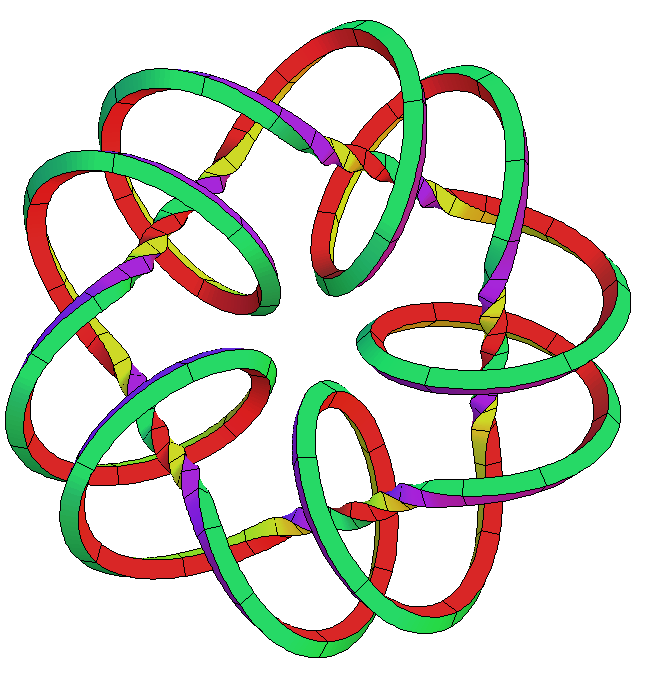
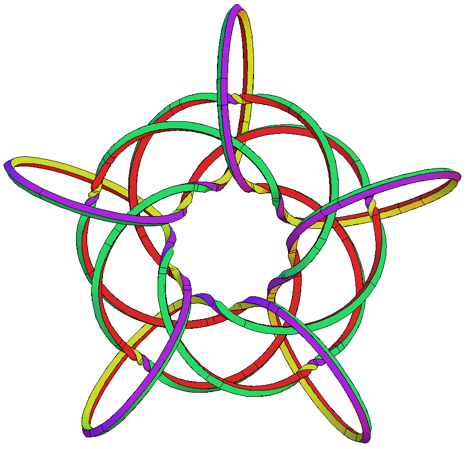
The canal surfaces on which these curves lie, look like a torus in the first case, but have heavy self-intersections in the other cases.
References
- [1] Hermann Karcher. Closed Constant Curvature Space Curves. https://arxiv.org/abs/2004.10284
- [2] Homepage of the program 3D-XplorMath. http://3d-xplormath.org/
-
[3]
Osculating circles moving along a ccc-autoevolute.
https://www.math.uni-bonn.de/people/karcher/MyAEvideo.html
Hermann Karcher unm416@uni-bonn.de
Ekkehard-H. Tjaden tjaden@math.tu-berlin.de